1. Introduction
Switching-on operations in the transmission grid create a number of risks resulting mainly from the emergence of high current values. Due to the short transient state, the thermal phenomena caused by the switching current are irrelevant, but the most important risks associated with the switching process are specified below:
The possibility of damage of the breaker due to exceeding its switching capacity;
The possibility of unnecessary excitation of distance-sensitive protections;
Hazards related to the possibility of damaging the windings of transformers or synchronous generators by the action of dynamic forces caused by the high value of peak switching current;
Stresses in the shafts of generating units, contributing to fatigue and reduction in their service life;
Threats related to the loss of stability of the power system (concerns connecting subsystems operating asynchronously and eliminating disturbances in the auto-reclosing cycle).
This article considers the problem of fatigue of shafts of generating units due to torsional oscillations caused by the switching of a transmission line with a significant difference of voltage phasors between connecting nodes [
1,
2]. On the basis of many computational tests conducted for real networks, authors concluded that the greatest problems may be caused by the impact of power surges on generating units [
3,
4,
5]. Therefore, the focus was on showing how the optimisation theory allows keeping the risk defined above in point 4 at a safe level.
It should be emphasised that the large voltage phasors difference between nodes in a synchronously operating power system is a phenomenon that can be taken as an indicator of the risk of system breakdown. This is also a warning that the internal structure of the system has weakened. This was the case on 4 November 2006, when the European system crashed into three unbalanced parts [
6]. The last attempt to strengthen the internal connections by closing the circuit breaker on the 380 kV Conneforde, Diele line (Germany) failed because, at the SPA angle exceeding 35 degrees, the synchrocheck system prevented the closing operation. Therefore, considering the connection operation with a high SPA value is a specific dilemma: on the one hand, closing the circuit breaker strengthens the cohesion of the system, but on the other hand, it may damage its components mentioned above in items 1–5. If so, it is advisable to look for the compromise solutions that define the safe border value of SPA, which at the same time will not be too restrictive. An attempt to search for such values of SPA angles is presented in the article.
The literature analysis [
7,
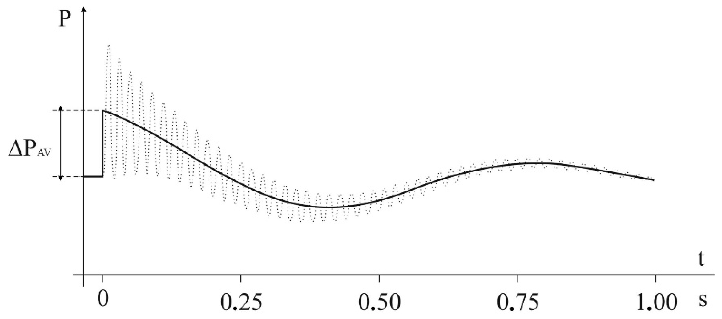
8] shows that line switch-on operation can be considered as safe for the generating unit shaft if the change in the active power caused by it meets the following simplified condition:
where
is the rated power of the
i-th unit. This relation should be fulfilled for
i = 1…
n, where
n is the number of all generating units working in the grid. The interpretation of the
value is given in the following
Figure 1.
A relatively easy task is to calculate power surges for the known operating state of the transmission grid, i.e., the actual value of the switch-on angle [
3]. The more difficult problem is to determine the maximum possible value of the standing phase angle at which the criterion condition specified in relation (1) is met.
In the present article, an attempt was made to solve this problem by using an original method of heuristic optimisation. The article consists of eight chapters. The first chapter contains an introduction to the subject of research and a justification of the purpose of the analyses. The second chapter presents a literature review on the problem of reduction in the SPA of transmission lines. The third and fourth chapters deal with the assumptions for the calculations. It formulates a computational problem. The fifth chapter describes the calculation method. The sixth chapter presents the CIGRE test network. The results of the calculations and the discussion of the results of the research and analyses are included in the seventh chapter. The conclusions are included in chapter eight. The main purpose of the article is to present a relatively simple calculation algorithm that can be used in practice in dispatch centers.
2. Literature Review
The subject of reducing the SPA of high voltage power lines in order to eliminate current surges, rebuild and restore the system to work is described in various ways in the literature [
4,
9,
10,
11,
12,
13,
14,
15,
16,
17,
18,
19,
20,
21,
22,
23,
24]. Both classical and heuristic methods are used, the aim of which is to minimise the negative phenomena caused by switching on the line when the difference of angles between the two poles of the breaker is too large. Changing the voltage angle difference is most often performed by changing the load distribution of generating nodes with a given load of consumers. Due to the temporary nature of the power system state sought, grid losses are not significant. It is important to effectively and safely minimise the angle differences. The word “effective” means the smallest possible load variation to achieve the required reduction in the SPA. The sources or loads that have the greatest influence on the voltage difference at the poles of the circuit breaker should be selected. The word “safely” means that there is no threat to the reliability of the power system operation. In article [
21], this issue was dealt with as a constrained optimisation issue. At the same time, a linearised model of the power system and linear programming were used for the calculations. First, it looks for states that meet the network constraints. Then the sources for which the required generation changes are minimal are found. Nonlinear programming to solve the problem of reducing the SPA of power lines was used in the article [
22]. The works [
15,
16] also applied linearisation of the power grid model. First, by an appropriate solution of the linear equations, a solution is found for which the sum of the squares of changes in the active power loads of generating units is minimal, and then this solution is corrected if there are exceedances of generating capacity limits. Similar considerations were presented in the article [
25], where the possibilities of reducing the load angle were extended by the possibility of unloading load buses. Based on the DC method, the analyses are performed in [
26]. The calculations are carried out in two stages. In the beginning, the power flow in the state before and after switching on the circuit breaker is determined. In the second step, for the generating buses, the voltage differences and their arguments in the state before and after the circuit breaker closure are calculated and treated as set points. On the other hand, analogous differences for load buses are treated as unknowns. Then, the power increases are determined, which constitute the sought changes in the generation of generating buses. The article [
18] assumes the search for such changes in the loads of generating and load buses. When a given network element is switched on, active power surges in all generators meet the condition (1). Since the subject of this article is consistent with the considerations of the authors of this work, it is presented more broadly. The calculations were performed in two steps. In the beginning, the optimal power flow (OPF) was determined, taking into account the network limitations, assuming the circuit breaker opening. The objective function described by Equation (2) was minimised:
where
and
are sets of generating nodes G and load buses L;
and
are weight factors;
is the active power in the determined state before closing the given circuit breaker;
is the active power in the initial state;
is the part of the load that is unloaded.
In the second step, such a power injection was calculated to satisfy the condition (1). The considered state is concerned the first moment after closing the circuit breaker, i.e., the state in which the generators experience an active power surge. The objective function described by Equation (3) was minimised:
where
is the set of generating buses subject to regulation,
is the weighting factor, and
is the fictitious power injection, which is minimised in successive iterative steps, so that Equation (4) is satisfied:
where (+) is the state at the first moment after the circuit breaker is closed,
is the set of buses
j that are neighbors of bus
i.
The purpose of the calculations is to find such values of
and
to satisfy the condition (1). The article uses the primal-dual interior point method. Similar considerations are presented in [
17].
As mentioned before, both classical methods, based on linearisation of the power flow task (DC method), and heuristic algorithms were used for the calculations. Articles [
4,
20,
23] concern methods based on artificial intelligence. The works described there can be included in the group of scientific and research works using heuristic optimisation methods to reduce the SPA of transmission lines. In [
23], both the generation change and the bus loads are used to reduce the SPA. A two-criteria objective function was used. The proposed method was based on a modified version of the genetic algorithm and tested on the IEEE 118 network. This article also uses the heuristic optimisation method described in point 5.
3. Description of the Problem—Details
Mathematical models and computer programs for electromagnetic simulation or electromechanical transients can be used to simulate the transient state caused by a difference of voltage phasors between network nodes to be connected. The simulation issues and the corresponding mathematical models are described in [
27]. However, a simplified analysis is also possible, as shown in this article. From the point of view of settings of devices for switching synchronism control, the “initial switching current”, understood as the effective value of the periodic component of the current just after closing the breaker, i.e., for the moment,
is important.
Similar to the calculation of the initial short-circuit current [
28], for the calculation of the initial switching current, synchronous generators should be mapped as for the subtransient state [
27,
28], i.e., by means of electromotive forces
with subtransient reactances, assuming that
. The values should be calculated for the given load state of the power system.
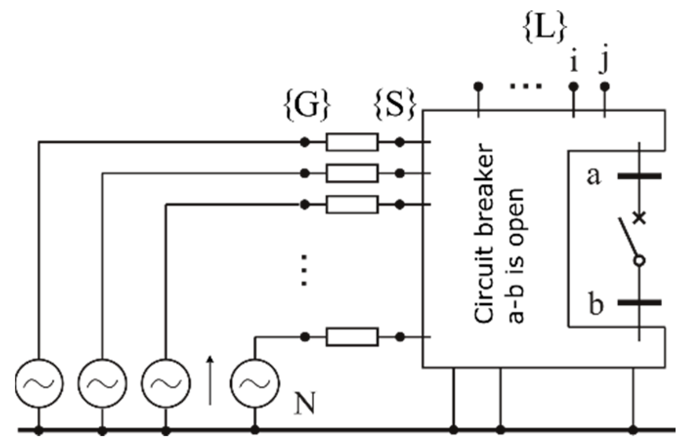
The creation of the network model for calculating the initial current is illustrated in
Figure 2. The set {S} is a set of buses to which the generating units are connected, while the set {G} is a set of fictitious generator nodes behind impedances of them. The set {L} is a set of load nodes. Loads are replaced by permanent admittances. The nodes a and b are the poles of the switched circuit breaker. Voltages at the poles of the breaker are marked, respectively,
,
and
. The difference in voltage arguments is marked as
.
In [
5], it was shown that all values necessary to calculate the current surge connected with performing switching operations could be determined by creating for the above model an impedance nodal matrix created in the same way as for short-circuit calculations [
28]. Changes in generator current caused by switching-on of the considered line can be then calculated from the following formula:
where
is the impedance of a given unit generator–transformer, and where
and
are the elements of impedance node matrix, while
is the initial switching current. The above current change is caused by the following power change in
i-th generator:
When using Formulas (5) and (6), it should be remembered that the underlined symbols refer to complex numbers in a common coordinate system.
In [
5], it was also shown that from the point of view of calculating the initial current
, the model of the analysed transmission grid (
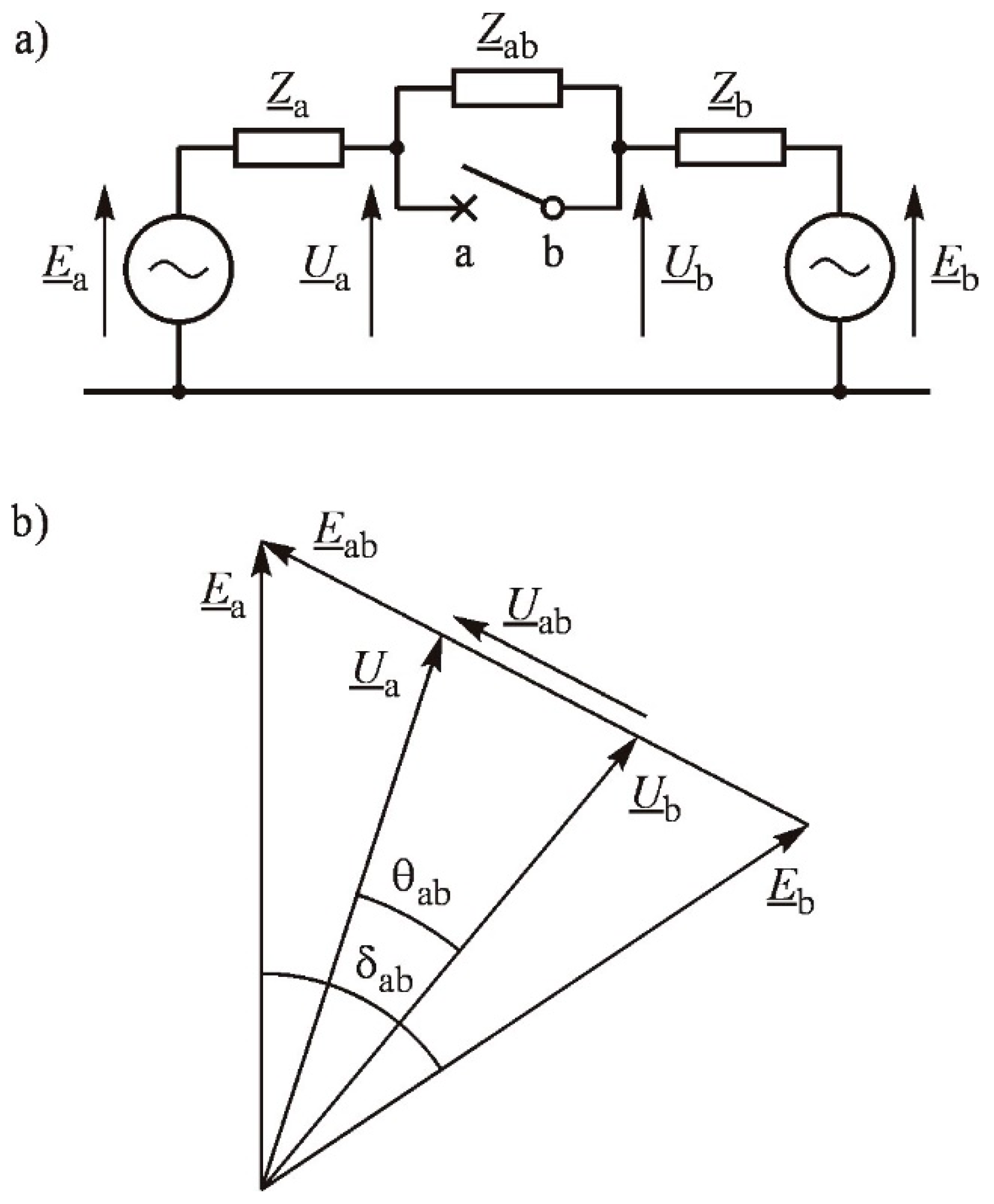
Figure 2) could be simplified to a simple substitute scheme, as shown in
Figure 3a.
In
Figure 3,
,
,
, and
describe the electromotive forces and impedances of substitute sources.
is the impedance of the substitute branch representing the connections of nodes
a,
b through the transmission network.
The initial switching current can be calculated by Thevenin’s theorem with the voltage value at the switched poles (
Figure 3b) and Thevenin’s impedance seen from
a, b nodes, with all voltage sources replaced by short circuits. This impedance (
Figure 3a) is given by the equation:
because looking from the side of nodes
a,
b, one can see impedances
and
connected in a series with each other and in parallel with
. For further analysis, the formula (4) describing Thevenin’s impedance can be transformed in the following way:
where
is a composite factor representing the influence of a longitudinal branch
on the value of Thevenin’s impedance.
Using the substitution diagram (
Figure 2a), the initial switching current
can be calculated as follows:
The
factor plays an important role in all further calculations. Therefore, in [
5], the analysis of the values assumed by this coefficient for the national transmission grid of 400 kV and 220 kV was performed. It was shown that for this network, the
coefficient is generally greater than unity and has a significant impact on the value of the switching current.
Knowledge of the initial value of the switching current (8) allows determining the initial value at the moment after switching on the transmission line, using formula (6). The formulae presented allow calculating power surges for each generating unit for a given load state.
With the settings of the devices for switching synchronisation control in mind, it is important to calculate the maximum limit value of the SPA , at which the value of the power change of i-th generator given by formula (6) will not reach the criterion value (1) for any of them.
In general, the following steps are required to calculate the maximum value of angle :
Change in load distribution among generating units to increase the angle by a small value ;
Calculation of new values of electromotive forces of individual generators in the changed state of load distribution;
Calculation of power surges due to switching on;
If the calculated power surges are less than the criterion value for return to point (a), and if the criterion value for any generator is met for an active power stroke, then complete the calculation and take the last value as the limit.
The main problem in such a procedure is how to determine the distribution of generating power between units (temporary unit commitment) so that it increases the SPA while limiting the power surges in generators associated with the switching on of a given network element (criterion (1)). The article proposes to use the optimisation algorithm to solve the problem.
4. Assumptions for Calculations
The problem is treated as an objective of nonlinear optimisation with limitations; control variables are continuous. The paper considers single-criterion objective functions.
The objective function is the difference of angles of voltage phasors in two network nodes during switch-on operation (SPA). The fact that these nodes are the poles of an open breaker is irrelevant here. If we assume that the nodes under consideration (
Figure 3a) are nodes
a and
b, then the function of the target will take the form of [
4,
29]:
where:
x = [PG1, …, PGm]—vector of active powers generated by the considered generation sources (vector of decision variables);
y = [PL1, …, PLi, QL1, …, QLi, PGn1, …, PGnn]—vector of uncontrolled active and reactive loads and generations (independent variable vector);
z = [U1, …, Ui, δ1, …, δi]—vector of phasors of nodal voltages (vector of dependent variables).
The optimisation task is to maximise the objective function while meeting the assumed limits.
By considering the above described objective functions together with the vectors x, y, and z, the optimisation task can be formulated in the following way:
The constraint assumptions are:
Limitation of decision variables (vector x) presented in Table 1;
Limits of dependent variables (vector z), which constitute permissible values of voltage at buses (generally maintained within the range from 0.9Un to 1.1Un);
Equal restrictions, which are nodal equations of power flow as well as equations of power balance in the power system;
Inequality restrictions, which constitute the permissible load capacity of power lines and transformers;
The limitation related to the power stroke criterion, expressed in relation (1).
The determination of the state vector
z for the known values of
x and
y vectors is one of the basic computational problems included in the computer analysis of power systems. This problem, known as load flow analysis (LF), is described in textbooks such as [
30,
31].
Many algorithms and computer programs were developed to solve this problem. Generally speaking, the components of the unknown vector
z (state variables) are determined from a system of nonlinear equations of the form
Each equation is formulated for a node of the analysed network so that the power balance for this node is equal to zero.
The nature of the issue under consideration (the power flow task) is such that the determination of the state vector elements takes place through an iterative process. The vector of decision variables consists of a continuous variable (active powers of sources). In the articles found in the literature (described in point 2), the DC method, i.e., linearisation of the power flow task, is most often used to solve similar problems. It is related to simplifications in the form of, for example, the lack of control over the reactive power flow. In order to eliminate these simplifications, it was decided to use one of the heuristic methods described in point 5.
5. Description of the Optimisation Method
The optimisation calculations were performed using the Algorithm of the Innovative Gunner [
29,
32], inspired by the selection of parameters of the artillery shelling so that the next shot precisely reaches its goal. The applied correction of the cannon parameters is different from the classic artillery theory. Hence, the term “innovative…” in the name of the method refers to a gunner. The innovativeness of the algorithm results from the fact of applying, at each step of the iterative process, the correction of the previous solution by means of specially selected multipliers [
29,
32] (dependence 16 and 17). This is a fundamental difference in relation to most methods [
33,
34,
35,
36,
37], in which, at the next step, the corrective element is added to the previous solution. Generally speaking, in most heuristic methods (nearly 100 such methods are defined and described [
38,
39,
40,
41,
42]), the iterative process of determining optimal values of the vector x components is similar, because most often in the next iterative step, which can be considered as additive correction, the following action is performed:
This means that at the next steps of the iterative process, the components of the decision vector are subject to “multiplicative” modifications, as opposed to “additive” modifications, which seem intuitive, regardless of the specificity of the algorithm used. Very simple functions gl1, …, glp and their arguments can be pointed out, which provide an effective solution to many optimisation tasks treated as benchmark models.
Experimentally it can be said that the best results will be achieved using two correction multipliers (
p = 2) and functions
g1 and
g2 of the same specific form, i.e.,
Variables
are not related to the physical theory of ballistics; however, because they are
angles chosen randomly in the process of drawing from the
range, they are called “corrective angles”. The drawing of angles
α and
β from the above-mentioned intervals are subject to a normal (or even) distribution, with a mean value of zero and a standard deviation, satisfying the relation
. The range of the random selection of “correction angles”
is narrowed during the iterative process according to the dependencies of geometric progress:
where the coefficient
a belongs to a range (0, 1).
Decreasing the acceptable range of angular variations α and β is justified by the coincidence of the algorithm to the optimal point. In the initial phase, the entire space is searched, and as the calculation approaches the end, the function area is increasingly limited in order to improve the value of the target function and to reach the optimum.
The choice of the function
g(
α) and
g(
β) is also crucial. They should be selected in such a way as to ensure that the decision variable is adjusted accordingly. According to these guidelines, the following functions were selected [
32]:
By adjusting the algorithm for a volley shot from
m cannons, it can be presented in a form that allows solving any optimisation tasks [
32]:
- 1.
Drawing of initial values of the components of the decision vector
;
- 2.
Finding the target function values for the start vector of the control variables, , ;
- 3.
Setting the iteration counter to i = 1, substitution ;
- 4.
Determining the scope of and ;
- 5.
Correction of the decision vector components by means of correction factors g(α), g(β):
solution j = 1, drawing of “correction angles” and according to a defined probability distribution, correction of the components of the decision vector
solution j = m, drawing of “correction angles” and according to a defined probability distribution, correction of the components of the decision vector
;
- 6.
Determining the values of target function for subsequent solutions 1…m, checking if the target function for the next solution is better than the solution from the previous iteration (if so, replace this solution with the current, better solution, and if not, leave it), identification of the q solution for which the function reaches the minimum value;
- 7.
Checking whether for the identified solution q the relation occurs; if so, then accepting it as the next decision vector in the iterative process, i.e., ;
- 8.
Verification of the stopping criterion (i + 1 = imax), end, or subsequent iteration (i = i + 1);
- 9.
End of calculation.
A significant part of new solutions should be generated in distant regions than the current best solution. This will make sure that we avoid the local optimum. The stop criterion is usually the maximum number of iterations, a predetermined number of iterations, or a fixed number of iterations without improving the best solution (sometimes called stagnation parameter).
Due to the existence of a population, the AIG algorithm is characterised by a large exploration of search space. The new solutions are diverse, which gives high effectiveness in avoiding local optimists. Other features of the AIG algorithm include universality, which is manifested by the fact that the algorithm is not associated with the properties of the problem.
The choice of the AIG algorithm to solve the present problem was dictated by the resistance to getting stuck in the local minima of the target function, large exploration of the search space, diversity of subsequent solutions, and a small number of control parameters.
Its effectiveness was proven in an article published in the journal Engineering Optimisation [
32] and monograph [
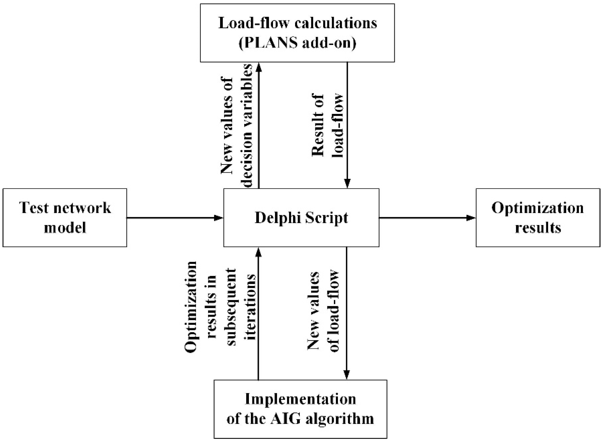
29]. Both of these documents present the calculations for problems in the field of mechanics and power engineering in terms of optimal power flow (OPF). The obtained results were compared with many other heuristic methods, considered the classic of heuristics. Appropriate software is necessary to solve problems in the field of electric power engineering. A program written in the Delphi environment was used for the calculations. The software includes an add-on in the form of a “calculation engine” of the PLANS program, used to determine power flows. Visually, it can be said that this add-on acts as an interchangeable computing engine that can be used in various applications. In this article, the Delphi environment was used, in which a program was written that connects with the PLANS program add-on and invokes the AIG algorithm. The course of calculations is shown in
Figure 4. After starting the main program in the environment, a remote connection with the flow program takes place. Changing the parameters of SEE elements or downloading calculation results is performed with the use of commands appropriate for a given programming environment. After running the AIG algorithm, the optimisation calculations follow, and the results are saved in a file.
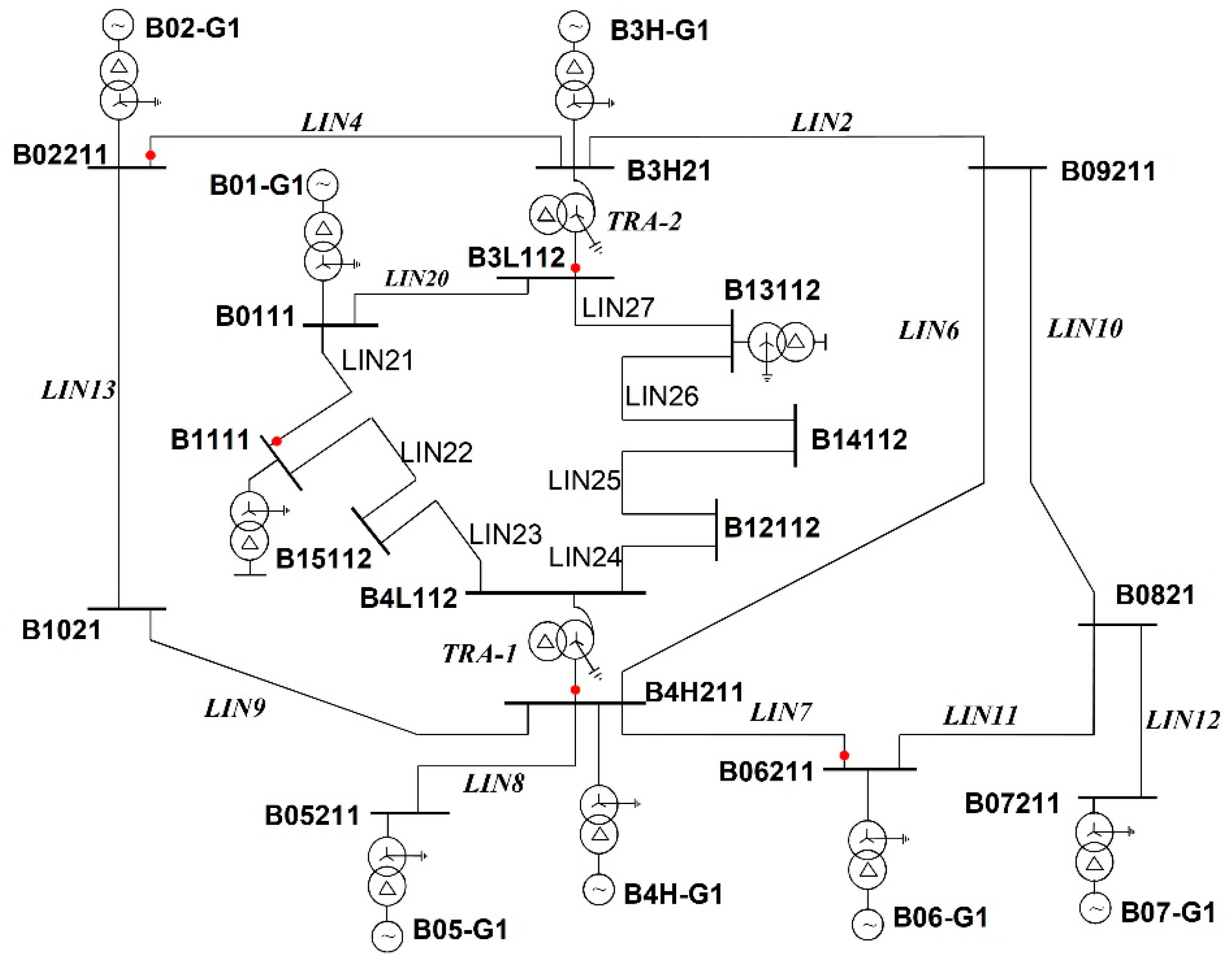
6. Test System
It is a modified version of the CIGRE Test System (
Figure 5). The voltage of that transmission network is 220 kV. The modification consists in including a fragment of a 110 kV distribution network to the system. The CIGRE test network consists of 7 generators, 17 nodes, 18 lines, and 2 transformers.
Table 1 shows the list of sources.
Table 2 shows the list of transmission lines with rated voltages.
7. Results and Discussion
For the optimisation calculations, 15 shots and 500 iterations were assumed using the AIG algorithm. It should be emphasised that the main objective of the discussed method is to determine the maximum SPA, which, in a given point of the network and in a given configuration, will ensure the possibility of safe performance of the switching operation from the point of view of the power surge criterion on shafts of generating units. Such an angle can be determined using the AIG algorithm and a properly defined penalty function (relationship (1)). However, the examples below present an algorithm that divides the process of determining the maximum (safe) SPA into two stages. In the first step, the maximum angle (SPA) that can arise between the two poles of the circuit breaker with a given network configuration is determined (
Figure 6a,b,
Figure 7a,b,
Figure 8a,b,
Figure 9a,b and
Figure 10a,b). This angle is a measure of the degree of risk associated with the performance of switching operations in a selected location. The second stage is the determination of the maximum value of SPA, safe from the point of view of power surges on shafts of generating units
Figure 6c,d,
Figure 7c,d,
Figure 8c,d,
Figure 9c,d and
Figure 10c,d).
There are forty switches in the network under consideration. Five characteristic switch locations were selected for the analysis, near and far from the power plant, in 220 and 110 kV networks, on lines, and at the transformer. The list of cases considered and the results obtained for them (in particular, the power surges determined for each of the generators) are shown below:
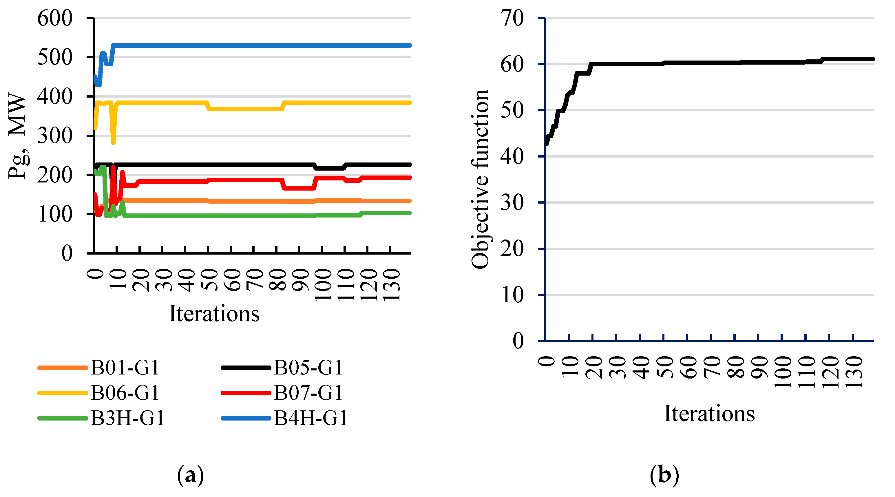
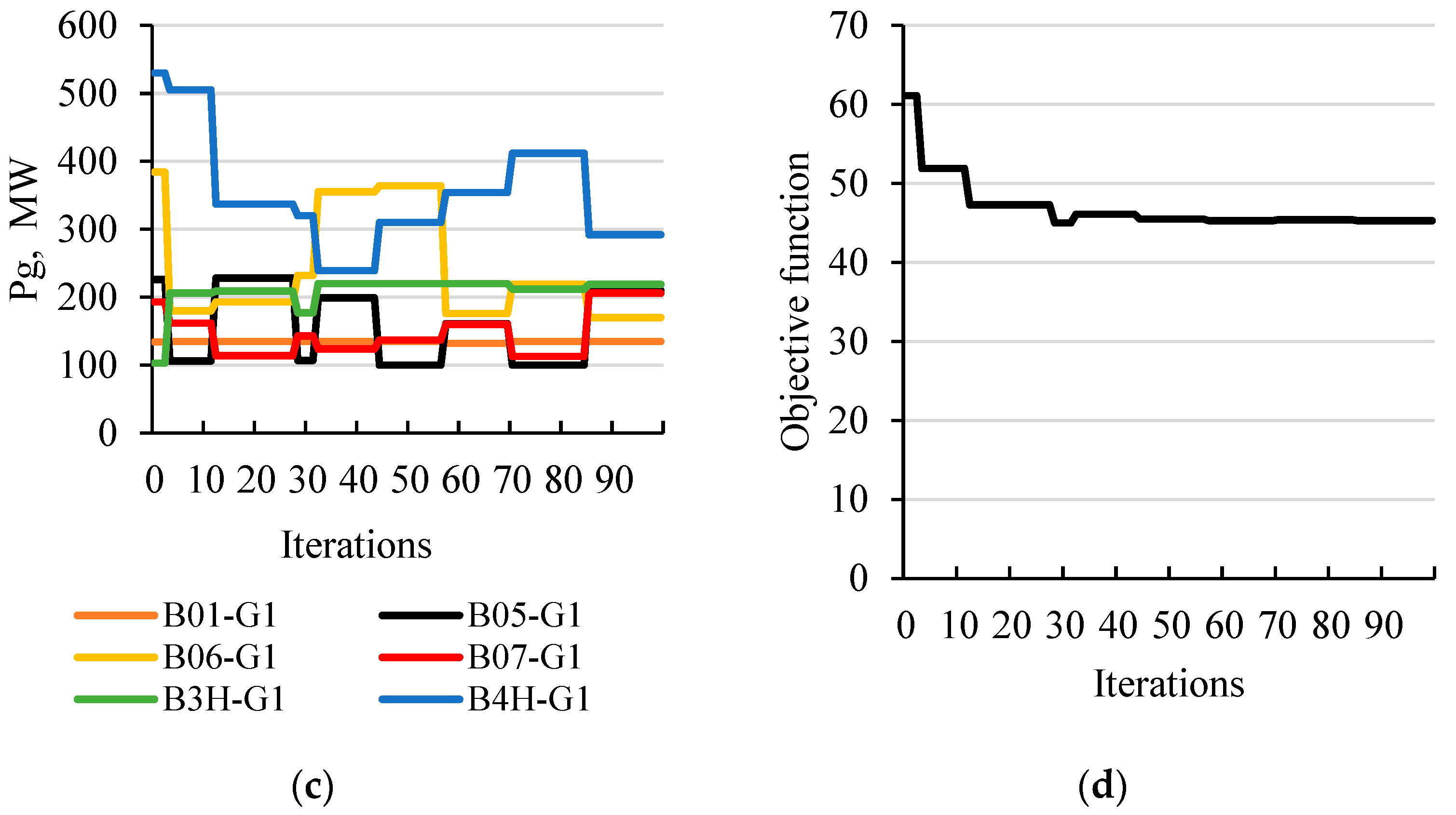
Case 1—the TRA-1 transformer located between B4H211 and B4L112 nodes is switched on; the connection point is located on the side of the B4H211 node, and the breaker at the B4L112 node is closed; the maximum safe value of the SPA was determined as 45.3° (global maximum value is equal to 61.1°).
Table 3 shows the list of sources with the values of power generated to ensure this safe maximum;
Figure 6.
The process of determining the maximum SPA for case 1; (a) changing the generation distribution to determine the maximum (global) SPA; (b) a graph of changes in the value of the objective function (maximum SPA); (c) changing the generation distribution to determine a maximum safe SPA; (d) graph of changes in the value of the objective function with the penalty function (maximum safe SPA).
Table 3.
List of sources with optimal capacity and expected values of power surges calculated for each generator.
Table 3.
List of sources with optimal capacity and expected values of power surges calculated for each generator.
| Name | Bus | Popt, MW | ΔP/Pn, % |
|---|
| B01-G1 | B01112 | 135 | 49 |
| B05-G1 | B05211 | 210 | 13 |
| B06-G1 | B06211 | 170 | 8 |
| B07-G1 | B07211 | 206 | <5 |
| B3H-G1 | B3H211 | 219 | 24 |
| B4H-G1 | B4H211 | 292 | 28 |
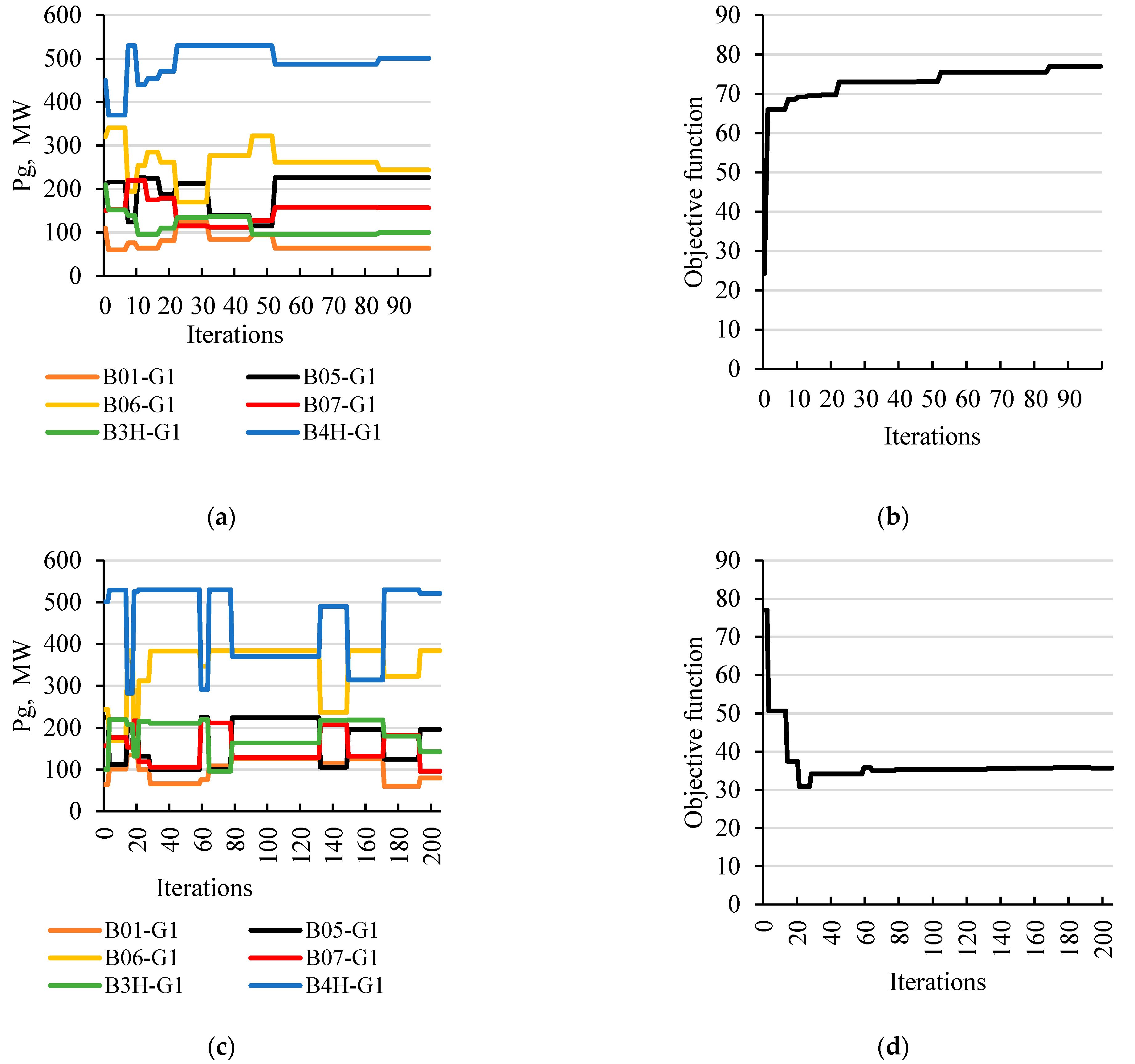
Case 2—line LIN4 between B3H211 and B02211 nodes is switched on; connection point is located on the side of B02211 node, and the breaker at B3H211 node is closed; the maximum safe value of the SPA was determined as 35.7° (global maximum value is equal to 77.0°).
Table 4 shows the list of sources and the values of power generated to ensure this maximum;
Table 4.
List of sources with optimal capacity and expected values of power surges calculated for each generator.
Table 4.
List of sources with optimal capacity and expected values of power surges calculated for each generator.
| Name | Bus | Popt, MW | ΔP/Pn, % |
|---|
| B01-G1 | B01112 | 80 | 8 |
| B05-G1 | B05211 | 196 | <5 |
| B06-G1 | B06211 | 384 | <5 |
| B07-G1 | B07211 | 96 | <5 |
| B3H-G1 | B3H211 | 143 | 49 |
| B4H-G1 | B4H211 | 521 | <5 |
Figure 7.
The process of determining the maximum SPA for case 2; (a) changing the generation distribution to determine the maximum (global) SPA; (b) a graph of changes in the value of the objective function (maximum SPA); (c) changing the generation distribution to determine a maximum safe SPA; (d) graph of changes in the value of the objective function with the penalty function (maximum safe SPA).
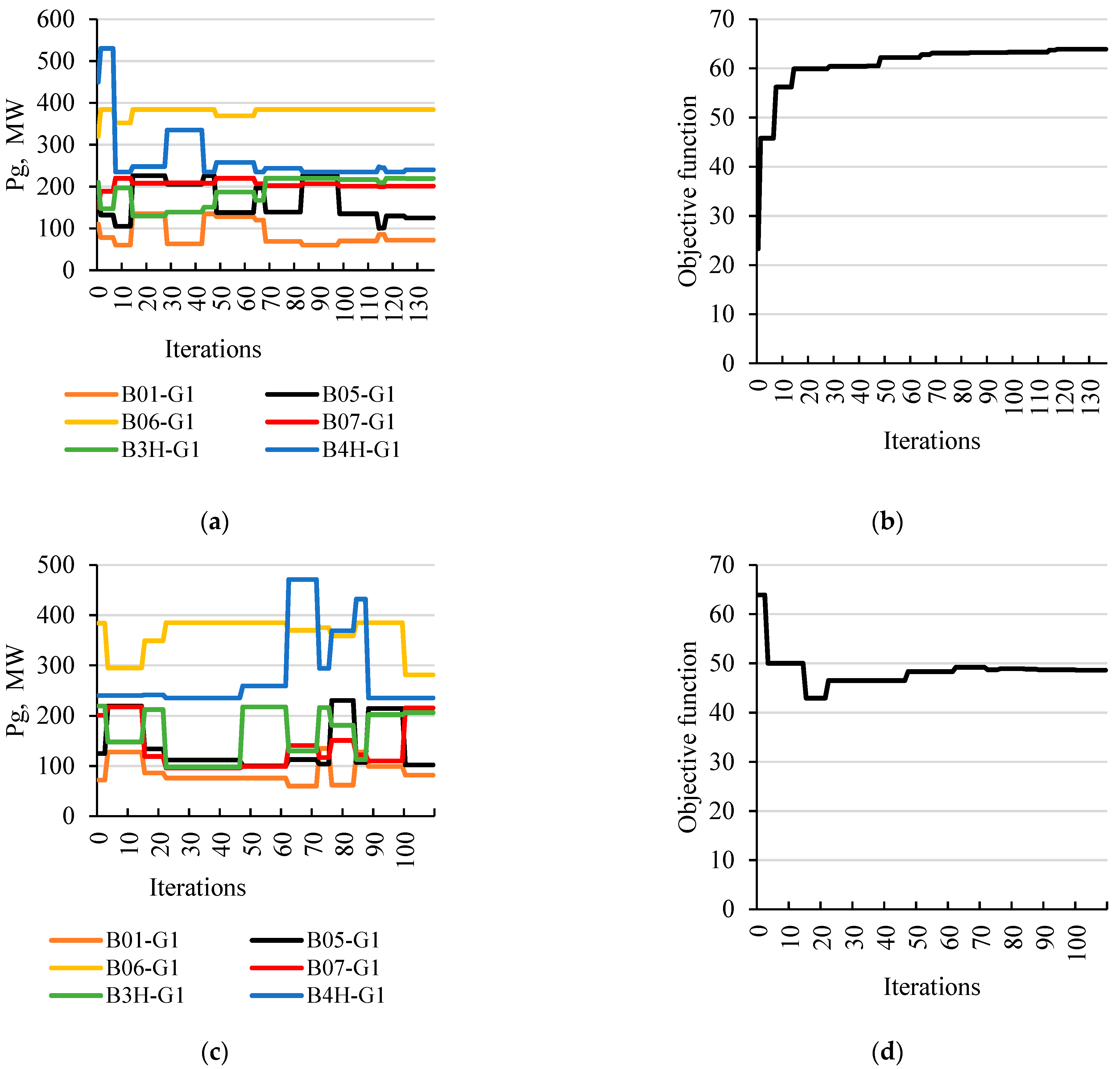
Case 3—line LIN7 between B06211 and B4H211 nodes is switched on; the connection point is located on the side of B06211 node, and the breaker at B4H211 node is closed; the maximum safe value of the SPA was determined as 48.6° (global maximum value is equal to 63.9°).
Table 5 shows the list of sources with the values of power generated to ensure this maximum;
Table 5.
List of sources with optimal capacity and expected values of power surges calculated for each generator.
Table 5.
List of sources with optimal capacity and expected values of power surges calculated for each generator.
| Name | Bus | Popt, MW | ΔP/Pn, % |
|---|
| B01-G1 | B01112 | 82 | 6 |
| B05-G1 | B05211 | 102 | 14 |
| B06-G1 | B06211 | 281 | 49 |
| B07-G1 | B07211 | 215 | 14 |
| B3H-G1 | B3H211 | 206 | 6 |
| B4H-G1 | B4H211 | 235 | 28 |
Figure 8.
The process of determining the maximum SPA for case 3; (a) changing the generation distribution to determine the maximum (global) SPA; (b) a graph of changes in the value of the objective function (maximum SPA); (c) changing the generation distribution to determine a maximum safe SPA; (d) graph of changes in the value of the objective function with the penalty function (maximum safe SPA).
In some cases, it is difficult to find the maximum value of the SPA for which relationship (1) is met. In this case, the power range of the unit (Pmax, Pmin) can be changed. This is described below.
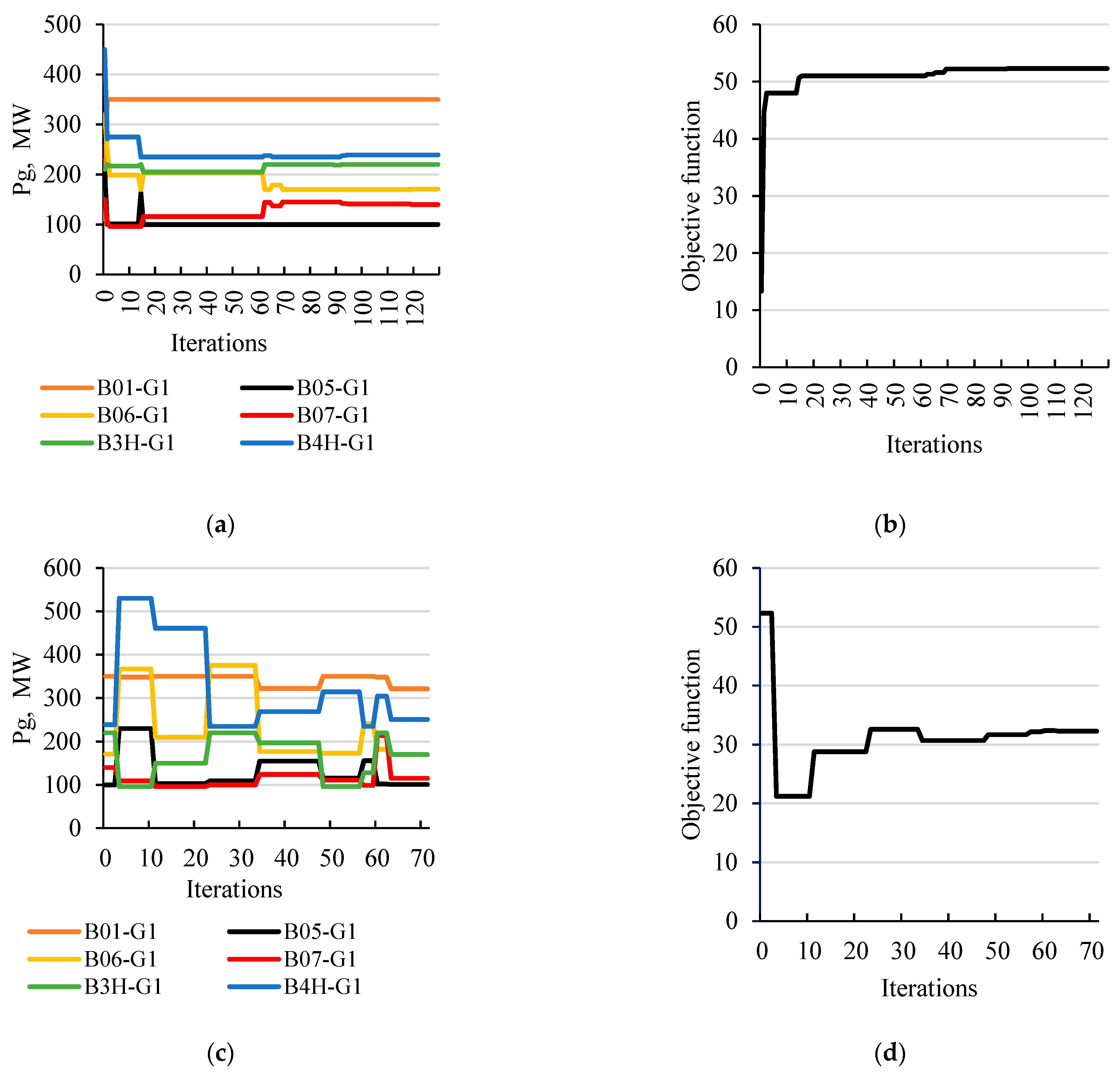
Case 4—It was assumed that the LIN21 line between B11112 and B01112 nodes would be switched on. The connection point is located on the B11112 node side, and the breaker on the B01112 node is closed. The control range of the B01-G1 generator was changed from 60 to 350 MW. The maximum safe value of the SPA was determined as 32.3° (global maximum value is equal to 52.3°).
Table 6 shows the list of sources with their optimal power generation values;
Figure 9.
The process of determining the maximum SPA for case 4; (a) changing the generation distribution to determine the maximum (global) SPA; (b) a graph of changes in the value of the objective function (maximum SPA); (c) changing the generation distribution to determine a maximum safe SPA; (d) graph of changes in the value of the objective function with the penalty function (maximum safe SPA).
Table 6.
List of sources with optimal capacity and expected values of power surges calculated for each generator.
Table 6.
List of sources with optimal capacity and expected values of power surges calculated for each generator.
| Name | Bus | Popt, MW | ΔP/Pn, % |
|---|
| B01-G1 | B01112 | 321 | 49 |
| B05-G1 | B05211 | 101 | 9 |
| B06-G1 | B06211 | 170 | <5 |
| B07-G1 | B07211 | 115 | <5 |
| B3H-G1 | B3H211 | 170 | 26 |
| B4H-G1 | B4H211 | 251 | 26 |
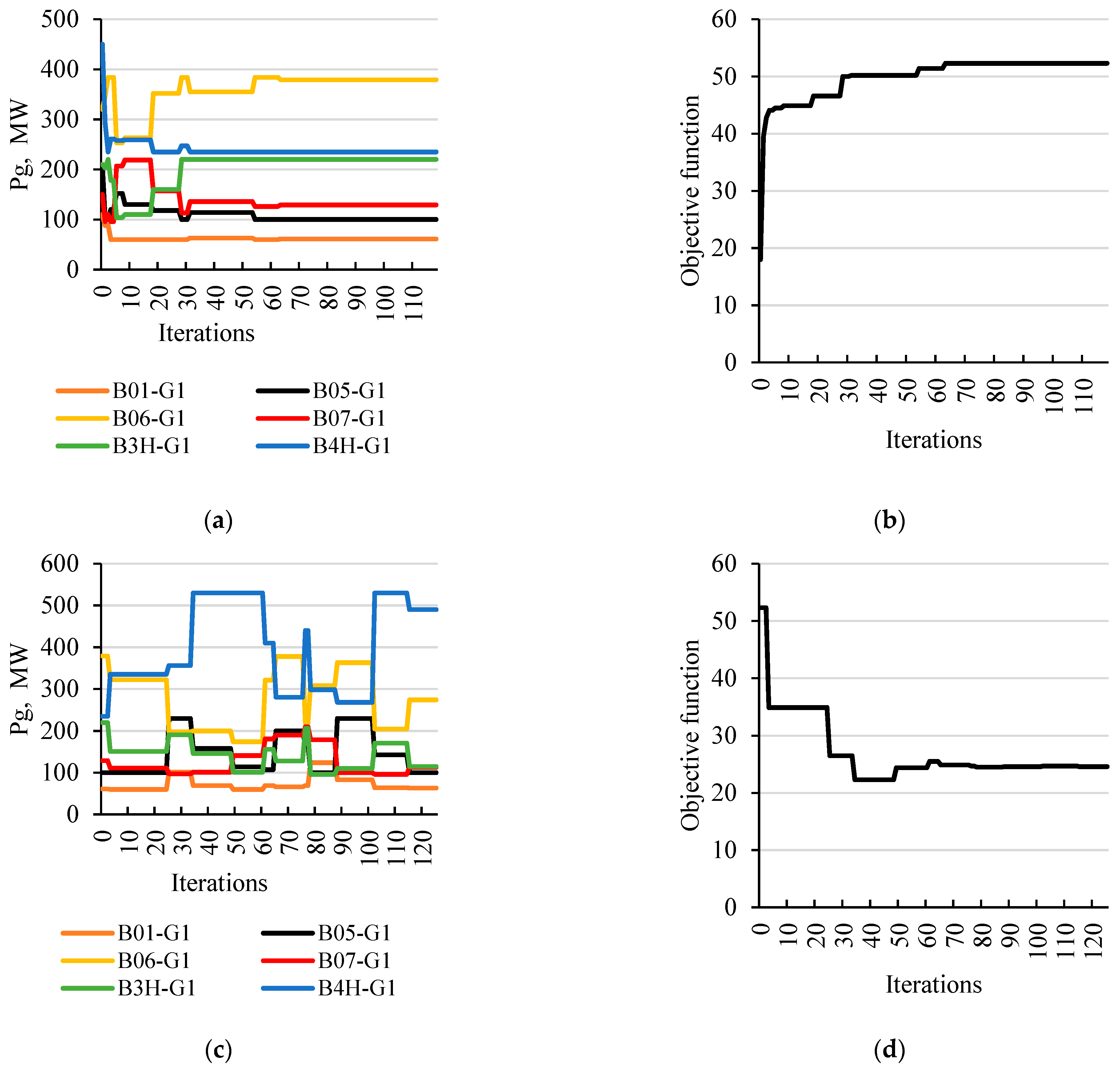
Case 5—the TRA-2 transformer located between B3H211 and B3L112 nodes is switched on; the connection point is located on the side of the B3L112 node, and the breaker at the B3H211 node is closed; the maximum safe value of the SPA was determined as 24.6° (global maximum value is equal to 52.3°).
Table 7 shows the list of sources with the values of power generated to ensure this maximum.
Figure 10.
The process of determining the maximum SPA for case 5; (a) changing the generation distribution to determine the maximum (global) SPA; (b) a graph of changes in the value of the objective function (maximum SPA); (c) changing the generation distribution to determine a maximum safe SPA; (d) graph of changes in the value of the objective function with the penalty function (maximum safe SPA).
Table 7.
List of sources with optimal capacity and expected values of power surges calculated for each generator.
Table 7.
List of sources with optimal capacity and expected values of power surges calculated for each generator.
| Name | Bus | Popt, MW | ΔP/Pn, % |
|---|
| B01-G1 | B01112 | 63 | 49 |
| B05-G1 | B05211 | 100 | 14 |
| B06-G1 | B06211 | 274 | 9 |
| B07-G1 | B07211 | 113 | <5 |
| B3H-G1 | B3H211 | 115 | 24 |
| B4H-G1 | B4H211 | 490 | 34 |
The computational process runs efficiently, the values of the control variables ensure the minimisation of the objective function is achieved practically after a relatively small number of iterations of the AIG algorithm. The above graphs show that it was practically enough for about 100 iterations to find the optimal solution. The test network used for calculations, considered in various operating states, justifies the necessity to use heuristic optimisation methods.
Table 8 presents the percentage values of the power surges for individual generators in the considered cases, in accordance with criterion (1). The values for which the power surges are close to the limit value are marked in bold. As can be seen, the criterion value (0.5
PnG) is not exceeded in any case. Therefore, it can be said that the solution of the optimisation task has fulfilled its goal: the maximum values of SPA were determined for which the power surges in the generators do not exceed the critical value of 0.5 of the rated power.
8. Conclusions
Operational or emergency shutdown of a transmission line or a transformer entails the necessity of reconnection and restoration of the transmission capacity of the network. Closing the breaker at high SPA may cause a large current surge, dangerous for elements of the power system. Therefore, actions must be taken to limit the current surge when switching on the transmission network elements.
One of the actions is to change the generation level of individual generating units while maintaining the balance of the generated and received power. From this point of view, such a distribution of generation levels that ensures maximum permissible SPA can be considered optimal.
Changing the generation levels for the time of switching operation is a momentary procedure, and after switching on the line, the previous state can be restored. The momentary change in the power will not affect the long-term overload of the system elements.
In the discussed situation, the speed and accuracy of the decision are valuable for counteracting the system failure. It is recommended that among numerous computer programs supporting the work of the power system operator, there are also algorithms of determining generation levels that maximise the value of the permissible SPA.
The problem presented in the article was effectively solved by means of the original heuristic algorithm. It proves that it is worth reaching for advanced mathematical methods, which support the operational activities of the dispatcher centers.


