Abstract
Increased integration of renewable energy sources brings new challenges to the secure and stable power system operation. Operational challenges emanating from the reduced system inertia, in particular, will have important repercussions on the power system transient stability assessment (TSA). At the same time, a rise of the “big data” in the power system, from the development of wide area monitoring systems, introduces new paradigms for dealing with these challenges. Transient stability concerns are drawing attention of various stakeholders as they can be the leading causes of major outages. The aim of this paper is to address the power system TSA problem from the perspective of data mining and machine learning (ML). A novel 3.8 GB open dataset of time-domain phasor measurements signals is built from dynamic simulations of the IEEE New England 39-bus test case power system. A data processing pipeline is developed for features engineering and statistical post-processing. A complete ML model is proposed for the TSA analysis, built from a denoising stacked autoencoder and a voting ensemble classifier. Ensemble consist of pooling predictions from a support vector machine and a random forest. Results from the classifier application on the test case power system are reported and discussed. The ML application to the TSA problem is promising, since it is able to ingest huge amounts of data while retaining the ability to generalize and support real-time decisions.
1. Introduction
The increasing penetration of renewable energy sources, coupled with the liberalized energy markets, gives rise to new challenges for safe, secure and stable power system operation. A growing share of renewables, i.e., wind and photovoltaic (PV) power plants, in the overall generation mix, combined with the simultaneous decommissioning of the conventional carbon-fired power plants, is putting the power system operation under increased stress [1,2]. Some of the principal operational challenges include: (1) reduced system inertia, (2) over-generation, (3) adequacy risks, (4) poor reactive power for voltage control, (5) grid congestion, (6) reduced frequency regulation, (7) steep residual load ramps, (8) negative residual load, (9) effectiveness of energy trading, and others. Particularly notable are the problems of reduced system inertia (when less generators with rotating mass are in operation) and adequacy risks (i.e., the lack of reserve margin to meet load at peak times) [3]. With the increased proportion of renewables in the generation mix, problem of the reduced system inertia will increase, with significant repercussions on the transient stability assessment (TSA) of the power system. Grid congestion may result from wind–solar production being concentrated within localized areas, while the steep residual load ramps are direct consequences of PVs operational restrictions. Aforementioned issues, among other things, exert new (and intensify existing) stresses on the stability and security of the (already strained) power systems. Moreover, they may exacerbate negative effects of severe faults, severe weather, and other internal and external power system disturbances [2,4]. Transient stability concerns are drawing attention of various stakeholders, as they can be the leading causes of major outages, which are accompanied by severe economic losses. For example, according to the Electrical Power Research Institute, power supply outages crisis create globally an economic loss estimates of $104 billion to $164 billion annually [2].
These developments are paralleled by the rise of “big data” in the domain of power system analysis. A development of the Wide Area Monitoring System (WAMS), within the power system, enables managing and utilizing huge numbers of dispersed phasor measurement units (PMUs), which provide high resolution data for supporting and enhancing reliability, stability and security of power systems. For example, according to Wang et al. (data from 2016), more than 2500 PMUs have been installed in Chinese North Interconnection, and each PMU collects more than 30 data features and refreshes them every 20 milliseconds [5]. This generates huge amounts of data that, potentially, can be mined for information. Namely, PMUs can directly collect various system dynamic information, including generator active and reactive power, rotor angle, various protection actions, and many others—many of which contain critical information for assessing the system security and stability [6]. Utilizing these PMU measurements data with the aid of artificial intelligence for a real-time power system TSA is currently a major topic of interest among researchers from academia and industry.
With all the recent advancements in power system monitoring, communication infrastructure, process control, and forecasting methodologies, it is now becoming possible to develop more advanced power system TSA schemes that can utilize available information for a safe, secure and stable power system operation. This development is heavily dependent on the use of advanced data mining and machine learning (i.e., artificial intelligence) techniques.
1.1. Literature Overview
Power system dynamic performance crucially depends on its ability to maintain a desired level of stability and security under various disturbances. The main focus of this paper is on the transient (or large signal rotor angle) stability, which can be considered as one of the most important types of power stability phenomena [2]. Figure 1 graphically presents a taxonomy of power system transient stability methods [7].

Figure 1.
A taxonomy of power system transient stability analysis methods.
Traditionally, the main approach to determine the stability of a power system was through a time-domain simulation (TDS), which is computationally cumbersome and does not meet requirements of modern systems [2]. Although direct methods reduce the computational requirements and provide stability margins, they have their own weaknesses [8]. Hybrid methods combine TDS with direct methods in different ways [7]. The focus here will be on the applications of different machine learning (ML) methods which are becoming predominant.
Authors in [9] applied a decision tree (DT) classifier to the transient instability prediction. DT is a weak learner with a strong tendency for overfitting. In order to overcome this deficiency, authors in [10] apply a three–stage DT based scheme for predicting the out-of-step conditions. Zhang et al. in [11] proposed a weighted random forest (RF) approach to the power system TSA. RF uses many DTs as base learners and removes many of their weaknesses. Baltas et al. in [12] presented a comparison of several different approaches.
Support vector machine (SVM) is another popular ML method for the TSA, which was used in [13,14] and, with certain improvements, in [15]. Several adaptations of the original SVM have also been proposed for the TSA: core vector machine [5] and ball vector machine [16]. Additionally, a neuro–fuzzy SVM approach was proposed in [17]. The SVM is confirmed as one of the best single models for tackling the TSA problem. It has a small number of hyperparameters which yield a stable decision boundary under many different circumstances. It can easily adapt to non-linearity using the kernel trick, and is generally fast to train.
Another popular approach to the TSA analysis is the artificial neural network (ANN), refs. [12,18]. Hou et al. in [19] proposed using a convolutional network, while Bahbah and Girgis in [20] proposed using a recurrent network, for solving the TSA problem. A review of different ANN based approaches (for the rotor angle stability control) is provided in [21]. Furthermore, specialized ANN architectures, developed specifically for the time-series processing, have also been applied to the TSA problem. These are based on special layer types: long short-term memory (LSTM) layer [22,23] and gated recurrent unit (GRU) layer [24]. These approaches generally do not require a separate features engineering step and can ingest raw time-domain signals. This completely removes any expert knowledge from the model building pipeline and the entire process is fully automated, which has its advantages and disadvantages.
A further extension of the ANNs, by stacking many layers, brings deep learning to this problem [25,26,27]. A hierarchical deep learning approach was presented in [28]. Autoencoders, as a special kind of ANN architecture, have also been applied to the TSA problem [29,30]. However, application of deep learning brings with it special problems of initialization, convergence, long training time, vanishing gradients, forgetfulness, dead neurons, and others [31,32].
By combining predictions from several (or many) individual models, in different ways, it becomes possible to build better performing and more robust models. This process is known as ensembling and can be, generally speaking, tackled in many different ways [33]: bagging, boosting, voting, stacking, blending, etc. Ensembles use individual qualities of different base models to create superior second-level models. Hang et al. in [34] propose boosting DTs as weak learners in creating ensemble for the TSA. Li et al. in [35] propose using gradient boosting machine. Baltas et al. in [36] propose boosting and voting ensembles for the TSA classification problem. Another approach to ensemble multiple models, using the soft voting, is proposed in [37] for the same type of problem.
Finally, there are still other avenues of attacking the TSA problem. These are variously based on statistical learning [38], mutual information theory [39], evolutionary computing [40], and others. Power system TSA is a rapidly evolving field, on the intersection of traditional power system analysis and artificial intelligence domains, under intense scrutiny by many researchers coming from different backgrounds and bringing their unique and valuable insights.
1.2. Contributions
The focus of this paper is on the utilization of various power system dynamic information, with a machine learning approach, for the power system TSA analysis. The contribution of the paper to the state-of-the-art is seen from two different perspectives: (1) data mining, features engineering and statistical post-processing of measured signals, and (2) feature space dimensionality reduction and TSA classifier building.
The first main contribution of the paper involves building a novel data set of time-domain signals for a benchmark test case power system. A sophisticate model of the IEEE New England 39-bus test case power system was built in the MATLAB/Simulink environment and utilized for generating a comprehensive database of PMU–type signals, emanating from different power system contingencies. Different load and generation levels of the system are covered, as well as all three major types of short-circuit events in different parts of the network. The dataset is 3.8 GB large and openly shared under the Creative Commons CC-BY license. Furthermore, a novel data processing pipeline is introduced for transforming this systematically generated dataset into the appropriate stochastic form, which captures natural class imbalance and statistical distribution of different fault types.
The second main contribution of the paper deals with introducing undercomplete denoising stacked autoencoder for reducing the dimensionality of the original feature space while preserving maximum information. This is reinforced by building a deep neural network (DNN) classifier for the power system TSA, by means of employing a transfer learning technique (with unsupervised pretraining). In addition, a classifier for the power system TSA is built using an ensemble learning approach. Ensemble uses the weighted soft voting for averaging prediction probabilities from two base classifiers: SVM and RF. These classifiers are compared on the same data set and their performance is measured using diverse metrics.
The rest of the paper is organized as follows. Section 2 introduces a data generation process, from the time-domain simulations of power system transients, and describes a data processing pipeline. Section 3 presents a ML architecture, which involves autoencoder, transfer learning and ensemble building, complete with classifier calibration and hyperparameters optimization. Section 4 presents results of the analysis of the test case power system with a discussion, which is followed by conclusions in Section 5.
2. Dataset Preparation
A large dataset of time-domain PMU signals is built using a highly-detailed MATLAB/Simulink [41] model (Section 2.1) of the IEEE New England 39-bus test case power system [42]. A fully automatic data processing pipeline follows (Section 2.2), with features engineering, statistical post-processing, stratified shuffle split and data scaling. Figure 2 presents a single-line diagram of the IEEE New England 39-bus test case power system that serves as a benchmark for the TSA analysis [6,29,30,37,42]. Power system features a total of 10 synchronous machines of different nominal powers, a number of transmission lines (TLs), three-phase power transformers and loads. Generator G1 represents an aggregation of large number of generators [42] and serves as a surrogate of the external power system. Each machine includes an excitation system control and a turbine governor.
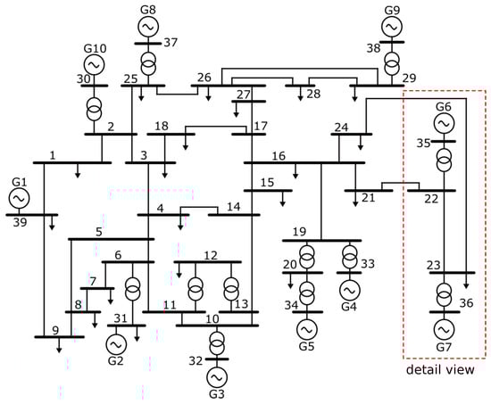
Figure 2.
A single-line diagram of the IEEE New England 39-bus test case power system.
2.1. MATLAB®/Simulink Test Case Set-Up and Simulation
Figure 3 presents a MATLAB/Simulink [41] model for the part of the power system from Figure 2, together with a detailed view of the generator model, including automatic voltage regulator (AVR), power system stabilizer (PSS) and turbine governor control. Generators are modeled as three-phase synchronous machines in dq rotor reference frame. A single-mass tandem compound steam prime mover, with speed regulator, steam turbine and a shaft is used for the steam turbine and governor. Hydraulic turbine with a PID governor system is used for hydro power plants. Different types of AVRs and exciters are used to model excitation systems [42]. Each generator can be equipped with multiple PSSs of different types (Figure 3). Loads are represented by three-phase parallel RLC branches. Three-phase –section line blocks are used to represent TLs. Interested reader is at this point advised to consult an excellent book by Kundur [43] for additional information.
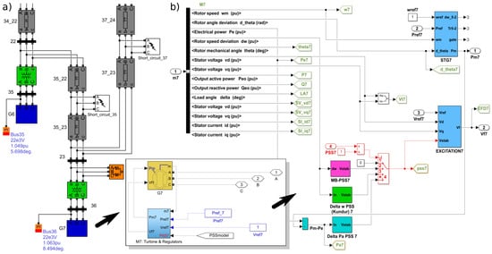
Figure 3.
A view of the MATLAB/Simulink model: (a) detail of the power system marked by a rectangle on Figure 2, (b) generator G7 model’s internal components and systems.
Flexibility of the test case power system is further enhanced by the use of specialized blocks and object-oriented programming. Three MATLAB® [41] workspaces are used to generate programming code that allows extensive modifications of the model after each simulation. The initial state of the system, along with the fixed system parameters, are set in the base workspace. Setting the variable model parameters, such as the duration and location of the short-circuit and the parameters that specify consumed power adjustment of the system, is enabled through the use of global workspace. Model workspace is used for selecting the type of short-circuit fault. The fault type, along with a desired timing of its onset, is manipulated using the specialized blocks which are deployed across the network. All TLs are divided into two flexible parts in order to facilitate programmatically changing the fault location. The whole process is driven by code and fully automated.
2.2. Features Engineering and Statistical Processing
Building of the dataset starts from a comprehensive set of systematic time-domain simulations (of post-contingency power system dynamics), using the nominal network topology with specific loading levels [44,45,46]. The consumed power was set at 80%, 90%, 100%, 110% and 120% of the basic system load levels (for different system load levels, both generation and loads are scaled by the same ratio). Then, for each load level, three different types of faults are assumed: (a) three-phase, (b) double-phase, and (c) single-phase short-circuits. They are located either on the busbars or on the TLs. When they are located on a TL, it was assumed that they occur at 20%, 40%, 60%, and 80% of the line length. The whole network from Figure 2 was, systematically, completely covered by all three types of faults. Furthermore, timing of the fault considers a moment on the reference voltage (phase A), obtained from the argument of the sine function at the time instant
where is the moment of the fault initiation (1 s), f is the frequency and is the phase angle [37]. Hence, faults are initiated after the power system steady state has been attained. At the same time, fault clearance times are associated with the time delays of the first and second zones of the distance protection relays, depending on the location of the fault. Relay protection of the generators was not considered. Bus faults, and those within the first zone of the distance protection, are cleared in 100 ms, while those falling within the second zone are cleared after 400 ms (time is measured from the moment of the fault inception).
For each contingency, a complete electro–mechanical transient simulation of the test case power system is carried out. The total number of systematic time-domain simulations required for the New England 39-bus test case equals 9360, which is a very large number for this level of model sophistication. The simulation run-time depends on the location and type of fault, its duration, pre-fault power system state, and other factors. The observation period of each simulation was set at 3 s, which is generally enough time to capture the nature of the transients under study. Saving of the time-domain signals to hard disk is taken with a time step of 1/60 s, which is consistent with the PMU measurements time resolution [45]. An Intel® Core i9 CPU with 16 GB of RAM was used to process this large number of simulations, which enabled the use of parallel workers. Parallel Computing Toolbox™ was used [41]. The total execution time was approximately 10 h and 30 min.
Simulations produce hundreds of measured quantities—as time-domain signals—for the network elements and machines (e.g., three-phase voltages and currents, active and reactive powers, rotor speeds and angles, etc.); Refs. [5,6,11,16,34,37]. Features that are used for the ML are extracted from these time-domain signals at two distinct time instants: (a) pickup time (pre-fault value) and (b) trip time (post-fault value) of the associated distance protection relays. These point-values, taken during each contingency, become raw features of the data set.
Table 1 presents select features, extracted from the time-domain signals, for the New England 39-bus test case power system [6,11,37,45]. All of the features are directly measured. There are no artificially engineered features. The majority of features are associated with measurements on the generators (both rotor and stator quantities). Phase angles of the voltage and current measurements have been disregarded, since it was found (following an in-depth feature analysis) that they are not very relevant [37]. It is clear that the number of features (sparingly chosen from a very large number of possibilities) is large, even for this relatively small test case power system. More importantly, it grows considerably with the increase in the number of buses and/or machines in the system and can easily become difficult to manage and process (curse of dimensionality). Hence, the main obstacle to successfully training any kind of ML model is found in controlling and/or reducing this large number of features without significant loss of information.

Table 1.
Features derived from the time-domain signals.
The use of supervised ML techniques further requires labeling of the collected samples. Transient stability index (TSI) is used here to indicate the preservation or loss of the power system stability [5]:
where is the maximum load angle difference between any two generators on the system. The TSI index provides a fast indication of the system (in)stability, based on the time-domain simulations [5,12,36,47]. If the TSI is positive, the system is in synchronism, otherwise it is in the out-of-step and thus unstable. Hence, TSI index determines a class label, where zero is used for the stable cases and one for the unstable cases.
Figure 4 graphically presents the data processing pipeline that follows this initial raw dataset building step. It consists of statistical post-processing of systematic simulations data (features), followed by the train/test data set split and concluded with a data scaling process.
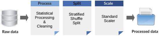
Figure 4.
An overview of the data processing pipeline.
A random set without replacement is selected from the population of systematically generated cases in such a way that the statistical distribution of different fault types follows the rule [37]: 70% single-phase, 20% double-phase and 10% three-phase faults. This brings dataset close to the overall (long term) statistical distribution of three different fault types in the power system. Moreover, it creates a stochastic dataset from the original population of systematic simulations. In addition, random selection preserves the natural imbalance in the allotment of the stable/unstable cases, which is a crucial aspect of the TSA phenomenon. It is expected that, with a larger power system, the imbalance of the final dataset to be very pronounced, which will have important repercussions on the subsequent ML models.
When the dataset is imbalanced (i.e., with a small number of cases belonging to the unstable class), a random sampling is not an option for splitting the data into training and test sets, since it would introduce a considerable sampling bias. Hence, a splitting strategy is needed that would preserve the class imbalance between the training and test sets. One such approach is known as the stratified sampling [48]. In the stratified shuffle split, a total population of training cases is divided into homogeneous subgroups (known as strata), and the right number of instances are randomly sampled (without replacement) from each stratum to guarantee that the test set is representative of the overall population.
Standardization of the dataset is a common requirement for many ML models. Hence, the last step of the data processing pipeline standardizes features in the training and test sets by removing the mean (i.e., centering) and scaling to a unit variance. Centering and scaling happen independently on each feature by computing the relevant statistics on the samples in the training set (only).
3. Machine Learning Architecture
Power system TSA of a real-world power system would impact huge parts of the power grid, which would involve thousands of measured time-domain signals (from which tens-of-thousands of features could be extracted). In addition, with data coming from the WAMS, it would be very difficult, error-prone and time-consuming to label many contingency cases. Hence, in order for the ML models to cope with this large amount of (mostly unlabeled) information it becomes necessary to reduce/filter the number of features, preferably using an unsupervised learning approach. This is seen as an indispensable data processing step of the classifier building pipeline [25,28,30,34]. Furthermore, since labeling of the contingency cases invariably produces (highly) imbalanced data sets, special care is needed during building and training of the subsequent ML models [36,37].
For effectively dealing with this two-pronged problem, the following two-part ML architecture is proposed: an undercomplete denoising stacked autoencoder, as an unsupervised deep learning model, is built and trained on the unlabeled data for intelligently compressing the feature space (Section 3.1), after which a binary classifier is built and trained using the labeled data. Two different classifiers are proposed and compared: (1) deep neural network classifier (Section 3.2) trained with a transfer learning approach, and (2) voting ensemble classifier (Section 3.3) built from SVM and RF using the weighted soft voting approach.
3.1. Undercomplete Denoising Stacked Autoencoder
Stacked autoencoder is a special kind of DNN for unsupervised (nonlinear) dimensionality reduction, which features an encoder and a decoder working in tandem [32,48,49,50]. Figure 5 presents a simplified illustration of the autoencoder model with an encoder function and a decoder function .
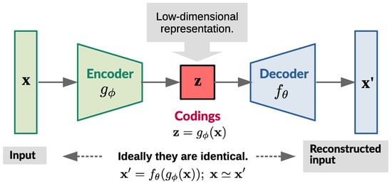
Figure 5.
A simplified illustration of the autoencoder model.
The low-dimensional encoding learned from input x in the central (bottleneck) layer is and the reconstructed input is . Nonlinear functions and are, essentially, two mirror–image DNNs, graphically presented in Figure 6.
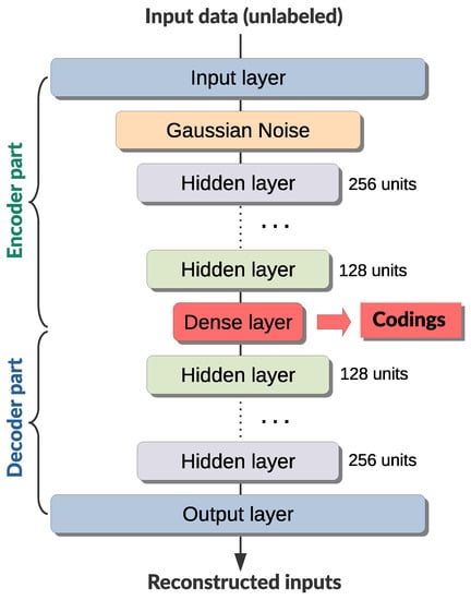
Figure 6.
An overview of the undercomplete denoising stacked autoencoder architecture.
The undercomplete stacked autoencoder, as can be seen, is composed of two back-to-back connected DNNs, namely, the encoder and a decoder networks. In other words, these two subnetworks need to have the same number of layers (and neurons per layer), in relation to the central (bottleneck) layer. Input and output layers need to have the same number of neurons as the dimension of the feature space. The encoder network’s hidden layers reduce the number of neurons (usually by halving) from the input layer, creating a funnel-shape towards the central layer which serves as an information bottleneck (the bottleneck layer captures a compressed latent encoding). Then, decoder network’s hidden layers increase them back again using the same sequence of steps.
The denoising stacked autoencoder, in addition, features a Gaussian noise layer immediately after the input layer, which injects noise into the input data (i.e., partially corrupts input data in a stochastic manner) and makes it harder for the decoder to reconstruct the inputs (i.e., learn input features). This reduces potential for overfitting and increases the robustness of the encoder–decoder pair, resulting in codings that preserve maximum information while reducing the dimensionality of the feature space [48]. Stacked autoencoder is superior to other dimensionality reduction techniques (such as the linear or quadratic discriminant analysis andprincipal components analysis), and it can be used for automatic features extraction [48,49].
Initial exploration of the autoencoder architecture—selection and tuning of hyperparameters (stacking of layers, selecting layer sizes, choosing neuron activation, regularization type and strength), scheduling and fine-tuning the optimizer learning rate, batch size, and other related issues—is tackled by means of the bandit-based optimization (Section 3.4.3). This provides automation at the expense of increased computational burden. Autoencoder is trained in the unsupervised manner, for a number of epochs, on the training set until there is no significant progress in the reduction of the Kullback–Leibler divergence loss [33]. Kullback–Leibler divergence measures the difference between the approximating and reference probability distributions, which is minimized under this loss. Adam (i.e., adaptive moment estimation) optimizer with an exponential decay of the learning rate and early stopping is employed during training, using a batch size of 32 instances. Exponential schedule decreases the learning rate from the initial value every steps with a decay rate of , which yields at the k-th step a learning rate of . Hidden layers are fully-connected, with the i-th layer given by , where neurons feature a ReLU activation function and –penalty regularization. Glorot normal initialization is applied to neurons weights [31]: , where and is, respectively, the number of input and output connections for the layer. A dropout layer can be used for additional regularization. Cross-validation with a stratified shuffle split of the training data set is used for model validation. Once the learning process terminates, the encoder part of the autoencoder is used for (nonlinear) dimensionality reduction of the features space (i.e., for encoding the training and test data sets).
3.2. Transfer Learning with Deep Neural Networks
Building a DNN classifier, by means of a transfer learning technique, encompasses reusing (i.e., cloning) the encoder part of the previously trained autoencoder and extending it with a stack of additional layers [32,48,50]. These additional hidden layers extend the encoder architecture and in-fact create a DNN classifier. Since this is a binary classifier, the last layer has a single neuron with a sigmoid activation function . Hidden layers are fully-connected, with neurons that feature a ReLU activation function with a Glorot normal initialization and –penalty regularization. Finally, a Monte Carlo dropout layer is introduced in order to facilitate estimating the confidence of the classifier predictions [48]. This confidence can be determined from a statistical distribution of classifier prediction probabilities that is constructed with a repeated Monte Carlo trials. Figure 7 graphically represents the essence of the transfer learning process of building a DNN classifier (with unsupervised pretraining).
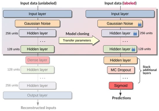
Figure 7.
Building a DNN classifier, by means of a transfer learning process, from the clone of the pretrained undercomplete denoising stacked autoencoder.
Supervised training of this DNN classifier, by means of a transfer learning approach, is a two-step process [48]:
- layers of the encoder part of the classifier architecture are frozen (which means that their weights cannot change during training) and the entire network is trained using labeled training data for a number of epochs, until there is no progress in the reduction of the binary cross-entropy loss [33];
- layers of the encoder part of the classifier architecture are un-frozen and optimizer learning rate is lowered for a second round of supervised training (i.e., fine-tuning) using the same labeled training data, again until there is no significant progress in the reduction of the binary cross-entropy loss.
Both rounds of training employ the adam optimizer with an exponential decay of the learning rate, and with a shuffled batch size of 32 instances. However, the fine-tuning phase uses considerably (i.e., 10 times) lower starting learning rate. Cross-validation on the training data set is used for model validation, along with an AUC binary classifier metric (Section 3.5) and early stopping, where validation set is created from the training set using the stratified shuffle split strategy. Furthermore, in order to cope with the class imbalance in the data, a class weight balancing is used during training to boost the representation (inversely proportional to the class frequencies) of the samples from the under-represented (i.e., unstable) class. After the DNN classifier has been further calibrated (Section 3.5), final predictions are made on the test set using the averaged prediction probabilities from a few hundred repeated Monte Carlo trials. This enables estimating classifier’s confidence about the class predictions.
All deep learning models are implemented in the Python programming language, using the TensorFlow 2 library from Google [51].
3.3. Ensemble Learning
Ensemble learning consists of pooling together predictions from a set of different base models to produce better and more robust predictions. The key to making ensembles work is the diversity of the set of base learners. For this reason, one should ensemble models that are as good as possible while being as different as possible. Ensemble learning is here used to build a meta-classifier, which combines and aggregates two very different models: (1) SVM classifier (Section 3.3.1) and (2) RF classifier (Section 3.3.2). Figure 8 graphically depicts the process of building this meta-estimator using the soft voting approach. Each base model is assigned a weight in the voting ensemble, which produces weighted average of probabilistic predictions from these individual classifiers. Ensemble learning is implemented by using the Scikit–Learn [52] Python library.
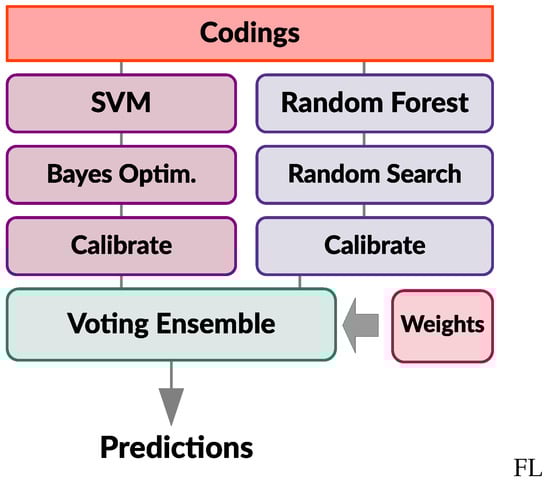
Figure 8.
An overview of the voting ensemble classifier built from SVM and RF base models.
Each base classifier is individually trained on the codings (training set) obtained from the autoencoder (Section 3.1) and produces independent predictions on the test set (i.e., outputs prediction probabilities, p). Since the dataset is imbalanced, each base classifiers uses class weight balancing during training, in order to put more weight on the samples from the under-represented class (by automatically adjusting weights inversely proportional to the class frequencies in the input data) [52]. Base classifiers are trained using the –measure as a scoring metric and individually calibrated on the training set (Section 3.5).
Voting ensemble (VE) classifier collects predicted class probabilities from the base classifiers, obtained on the test set (from which a small portion is reserved for validation), and computes their weighted average . A final label is derived from the class with a highest average probability. Individual classifier weight () contributions to the ensemble are computed by solving the following constrained optimization problem:
which features a negative log-likelihood of the classifier , where is a true class label and is the probability estimate from the classifier (on the validation set); with being the number of base models. Solution of the optimization problem in (2) is found by using the sequential least-squares programming routine from the Scipy [53] Python library.
3.3.1. Support Vector Machine Classifier
SVM classifier is a supervised learning method that uses a subset of training points (called support vectors) and kernels in constructing the decision function, which for a given sample x can be written as follows:
where summation of sample pairs is over the space of the support vectors (SV), while is the selected kernel function. Unknown coefficients and b are to be determined by solving the following optimization problem [33]:
where C is the penalty that acts as an inverse regularization parameter, while is a slack variable and n is the number of samples. Introduction of a slack variable, which allows some samples to be at a distance from their correct margin boundary, is necessary to cope with otherwise infeasible constraints of the optimization problem. Here, a radial basis function (RBF) kernel is used [33]:
The penalty (C) and the kernel coefficient () for the RBF, as two crucial hyperparameters of the SVM, are optimized using the Bayesian optimization (Section 3.4.2), with a cross-validation on the training set. It should be noted that penalty interacts quite strongly with the kernel parameters. Further details of the SVM implementation and solution to (4) can be found in [33].
3.3.2. Random Forest Classifier
RF classifier is an ensemble learner built using randomized decision trees. DT is a non-parametric supervised learning method that makes predictions by learning simple decision rules inferred from the data features [33]. DT classifier constructs a binary tree using the feature and threshold that yield the largest information gain at each node. It consists of branches and leafs, and is usually grown to full size, after which a pruning step is often applied to improve its ability of generalization. The complexity and size of the tree can be controlled by the appropriate hyperparameters [52]. DT classifier is prone to overfitting (i.e., it has a low bias but a high variance).
RF classifier creates a diverse set of these DT classifiers by introducing randomness in the classifier construction (perturb-and-combine) and subsequently aggregates their predictions by averaging (probabilistic) predictions of the individual DTs. In RF, each DT in the ensemble is built from a sample drawn with replacement (i.e., bootstrap sample), from the training set. Furthermore, when splitting each node during the construction of a tree, the best split is found either from all input features or from its random subset. The purpose of introducing these two separate sources of randomness is to decrease the variance of the RF, improve its predictive accuracy and control the overfitting. The process of building a forest of trees can be controlled by a number of hyperparameters [52], which are optimized using a random search with a k-fold cross-validation on the training set (Section 3.4.1).
3.4. Hyperparameters Optimization
A crucial part of the ML model training process involves the hyperparameters optimization, which can be carried-out using different approaches [48,50]. Three methods will be briefly presented hereafter: (1) random search, (2) Bayesian optimization, and (3) Bandit-based optimization. Each optimization method defines a configuration space (of hyperparameters) and uses a particular search algorithm.
3.4.1. Random Search
Random search is one of the simplest methods for the ML model’s hyperparameters optimization. It is suited for situations where there are large numbers of parameters of different types (continuous with and without bounds, discrete that are ordered or not, conditional, etc.) [52]. The random search method only presupposes the individual statistical distributions (either continuous or discrete) for each of the hyperparameters. Then, during a fixed number of iteration cycles, parameter values are randomly sampled from these specified distributions. With each combination of sampled hyperparameters, a model is trained using the k-fold cross-validation approach. The best combination of sampled hyperparameters are retained after the iterative process is finished. This method is superior to the grid search, but less informed than the Bayesian optimization.
The following hyperparameters of the RF classifier are fine-tuned using the random search [52]: number of trees, maximum depth of tree, number of samples required at a leaf node, minimum number of samples required to split an internal node (all from discrete uniform distributions); fraction of samples for training each tree, fraction of features to consider, threshold for early stopping in tree growth (all from continuous uniform distributions); function to measure the quality of tree split (from a discrete set); bootstrap sampling binary variable.
3.4.2. Bayesian Optimization
Bayesian optimization (BO) features a Gaussian process prior and evidence to define a posterior distribution over the space of functions, where optimization follows the principle of maximum expected utility [54]. It imposes limits on the hyperparameter space of the model, which can be very wide, and uses guided search through this hyper-space using the cross-validation on the training set [55]. It does not impose specific distributions on the hyperparameters. This approach is suited for the ML models that are expensive to train and have a small number of real-valued hyperparameters.
The BO rests on the underlying Gaussian process (GP) that can be defined as [33]:
which stipulates a zero mean and here implements a Matérn kernel:
with , where ℓ stands for the kernel width, while is the Gamma function and is the modified Bessel function. At the same time, the upper confidence bound (UCB) is selected for the acquisition function (AF) of the BO, as follows [33,54]:
where is the parameter of the AF which can be fine-tuned, while is pre-selected by the user and controls the exploration–exploitation trade-off. The role of the acquisition function is to guide the search for the optimum. Typically, high acquisition corresponds to potentially high values of the objective, whether because the prediction is high, the uncertainty is large, or both. Maximizing the AF is used to select the next point () at which to evaluate. The AF from (8) balances the trade-off of exploiting and exploring the hyper-space of potential values (through the parameter). When exploring, it chooses points where the surrogate variance is large. When exploiting, it chooses points where the surrogate mean is high [54].
The predictive (posterior) distribution can be described by the following update rule [33,54]:
with:
where and are, respectively, a set of previously processed points (i.e., hyperparameters) and their associated values; K is the kernel matrix of the processed points and k is the vector of kernel values at the next point . The iterative process is started from the randomly selected initial hyperparameter values and stopped after the predefined number of iteration steps. Additional implementation details can be found in [54].
During each iteration step, a ML model with the most-current values of hyperparameters is trained on the part of the training set and validated on the held-out part, using the cross-validation approach. The best combination of hyperparameters are retained after the iterative process is finished.
3.4.3. Bandit-Based Optimization
A so-called “hyperband” bandit-based optimization is employed, which speeds-up random search through the adaptive resource allocation and early-stopping [52,56]. This method is well suited for dealing with large number of hyperparameters of different types. Hyperparameter optimization is formulated as a pure-exploration non-stochastic infinite-armed bandit problem, where a predefined resources such as iterations, data samples, or features are allocated to randomly sampled configurations. The hyperband algorithm balances the number of hyperparameter configurations n given some finite budget B of resources (i.e., n versus ), by considering several possible values of n for a fixed B [56]. Associated with each value of n is a minimum resource r that is allocated to all configurations before some are discarded; a larger value of n corresponds to a smaller r and hence more aggressive early-stopping strategy. Hyperband, in addition, employs and extends on the successive halving algorithm, which essentially works by (1) allocating a budget to a set of hyperparameter configurations, (2) evaluating the performance of all configurations, (3) throwing out the worst half, and (4) repeating until a single configuration remains [52,56]. The hyperband algorithm iterates over different values of n and r and for each pair invokes successive halving algorithm, yielding a high-performing configuration (according to the selected loss metric) after a number of iterations. Additional implementation details can be found in [56].
3.5. Performance Metrics and Classifier Calibration
Transient stability index, which indicates preservation or loss of system stability, has been introduced to label the samples (Section 2.2) as belonging to the stable or unstable class. With a data set that features class imbalance, and when considering unequal miss-classification costs, accuracy of the binary classifier alone cannot be considered a valid metric for reporting its performance [33]. All types of classification errors need to be considered, as well as their repercussions on the subsequent decision making process.
Precision (i.e., positive predictive value, PPV) and recall (i.e., true positive rate, TPR), as derived measures, capture the important trade-off that the classifier needs to perform, since there is an inverse relationship between them (where it is possible to increase one at the cost of reducing the other). Precision is the ratio:
where is the number of true positives and the number of false positives. True positives, in this setting of transient stability analysis, are results where classifier correctly predicts unstable cases. False positives are, at the same time, results where classifier falsely predicts that the cases are unstable which are in fact stable (i.e., false alarms). Recall is the ratio:
with being the number of false negatives. False negatives are results where classifier falsely predicts that the cases are stable which are in fact belonging to the unstable class. This kind of error is worse, in terms of the repercussions on the subsequent decisions, than the false alarms. Classification accuracy is defined as:
with being the number of true negatives (i.e., results where classifier correctly predicts stable cases). Accuracy, however, can be a misleading metric for imbalanced data sets.
Both precision and recall are scored in the range between zero and one. A precision score of for the unstable class means that every item labeled as belonging to this class does indeed belong to it (but it says nothing about the number of items from this class that were not labeled correctly). A recall of for the unstable class means that every item from this class was correctly labeled (but it says nothing about how many items from the stable class were also incorrectly labeled as belonging to this class). For the TSA analysis, classifier’s recall score can be seen as more important than precision. Individual scores (PPV and TPR) can be further combined into a single metric, the score, which is a weighted average of the precision and recall:
In addition, , which can also be defined in terms of the Jaccard coefficient (JC) as . However, this measure ignores true negatives () and can also be misleading for unbalanced classes. A better approach would be to use the Matthews correlation coefficient (MCC):
which is generally regarded as a more balanced measure for the class imbalanced data sets. Matthews coefficient ranges between and . A coefficient of represents a perfect prediction, 0 no better than random guessing and indicates a total disagreement between prediction and observation. Finally, the Brier score (BS) is reported, which measures the accuracy of probabilistic predictions:
where and , respectively, denote the i-th sample’s label and probability of being classified into the positive class, while n is the number of samples. The Brier score, as a mean square error, is lower with better calibrated predictions (but strictly positive).
Classifier performance can be further gauged by the area under the receiver operating characteristic (ROC) curve (i.e., the so-called ROC–AUC score) [52]. A complementary comparison, which better emphasizes unequal miss-classification costs, is possible using a so-called detection error trade-off (DET) curve, which is plotted using a normal deviate scale [52]. This curve allows comparing classifiers in terms of false positive rates (FPR) and false negative rates (FNR) they produce.
Finally, classifier calibration deals with choosing the optimal probability threshold level in relation to the balance between the precision and recall, or in terms of false alarm vs. missed detection costs. In other words, this threshold level depends on the importance of different classifier errors ( vs. ) on the subsequent decisions and needs to account for the class imbalance.
4. Results of New England 39-Bus Case Study
A subset of the obtained results will be presented here, due to space concerns. The autoencoder first reduces the dimensionality of the feature space down to 16D, which is considered sufficiently low-dimensional representation for this case study [9,12,37]. Next, the DNN classifier is trained using a two-step process (Section 3.2), which follows cloning and extending the encoder part of the (pretrained) stacked autoencoder. Consequently, Figure 9 presents the binary cross-entropy loss values during both phases of the DNN classifier training. A training and validation loss values (using cross-validation) are provided as a function of the training epoch. The loss value reaches a plateau after certain number of epochs, which is detected by the early stopping [51], indicating convergence of the model.
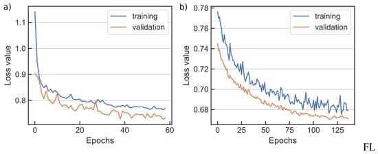
Figure 9.
Training and validation loss values for a DNN classifier during transfer learning: (a) network training phase, (b) network fine-tuning phase.
A voting ensemble classifier (Section 3.3) was built from individually trained SVM and RF classifiers, each cross-validated on the training data set (from the codings of the autoencoder). Prediction probabilities from the SVM and RF classifiers were averaged (using weighting) by means of soft voting. A weight ratio of approximately 60:40 in favor of the SVM was obtained from solving Equation (2), confirming that it is a better classifier. Individually trained classifiers were calibrated using the precision/recall curves, which are graphically presented in Figure 10. A threshold level was marked, for each of the classifiers, at which the highest precision and recall combination could be simultaneously achieved. Threshold defines the internal level at which the probability (of the unstable class) was set, and its optimal value often differed from the baseline.
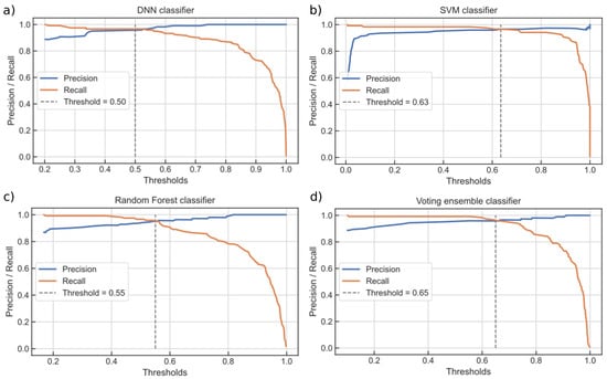
Figure 10.
Precision/recall trade-off curves for each of the classifiers: (a) DNN classifier, (b) SVM classifier, (c) RF classifier and (d) VE classifier.
The inverse–proportional relationship between the precision and recall was evident. It can be seen that the recall often started to fall (dramatically) after a certain threshold level. It is also clear that one could not increase the precision of the classifier without reducing the recall, and vice–versa. Hence, the different importance that the precision and recall have on the subsequent decisions featured prominently in the classifier calibration step. Fine-tuning of the threshold value needed careful consideration of the unequal miss-classification costs. For example, it can be seen that the VE classifier threshold could be further adjusted for an increased recall at the expense of a slightly reduced precision.
The classifier produced a prediction probability for each sample in the test set, which was converted (based on the threshold level) to the statement of belonging to the unstable class. Figure 11 presents a confusion matrix for each of the three individual classifiers. A confusion matrix features (off diagonal) the number of false positive () and false negative () errors the classifier produces on the test data set (Section 3.5). Particularly important in the setting of power system TSA were the false negatives. The DNN and the SVM classifiers had the same number of false negative errors, while the RF classifier performed only slightly worse. These results could vary between runs due to the stochastic nature of the models (which did not influence the final classifier decisions).
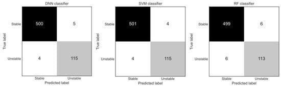
Figure 11.
A confusion matrix for the DNN, SVM, and RF classifiers, determined on the test set.
Moreover, since the DNN classifier yielded a (final) prediction probability by the process of averaging prediction probabilities from several hundred Monte Carlo trials (Section 3.2), this particular classifier (unlike others here) in the process generated a full probability distribution (instead of a single value) of the prediction probability. This probability distribution is graphically displayed in Figure 12 for a few selected cases from the test set. The probability distribution is depicted with a “boxplot” with a superimposed “strip plot” (overlaid on the boxplot to give a visual clue to the distribution shape). It can be seen that the threshold level of the DNN classifier cut through the statistical distribution. Confidence of the DNN classifier in the predictions was clearly evident. For example, the classifier was much more certain about Case 2 belonging to the stable class then about Case 3, which could reveal obscure details about particular cases that can be important for understanding (and improving) classifier performance.
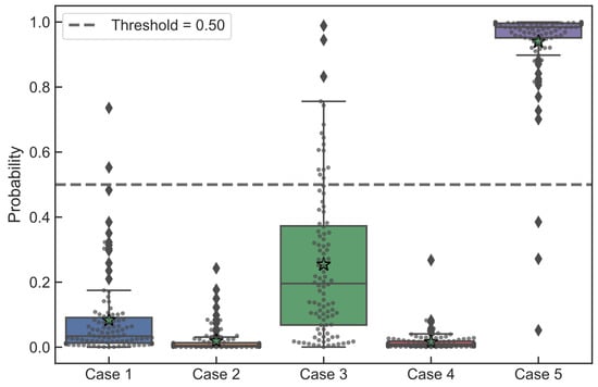
Figure 12.
Monte Carlo determined statistical distribution of prediction probabilities from a DNN classifier for a few select cases (Cases 1 through 4 belong to the stable class, while the Case 5 belongs to the unstable class). Boxplot: bottom and top lines of the box represent, respectively, first (Q1) and third (Q3) quartiles; the line inside the box is the median value (Q2); “whiskers” represent the lowest datum still within the 1.5 IQR (interquartile range) of the lower quartile, and the highest datum still within the 1.5 IQR of the upper quartile; diamond points outside the whiskers represent outliers; “star” indicates the mean value.
A further comparison of the classifiers performance on the test set could be analyzed by means of the ROC and DET curves. Figure 13 presents ROC and DET curves for each of the classifiers, including the voting ensemble. The ROC curves are here depicted in the coordinate system of precision and recall scores, with isolines of constant –metric values superimposed for reference. This is an alternative presentation of the traditional ROC curve that better emphasizes the importance of the class imbalance (the better the classifier is the closer is its curve to the upper-right corner). A classifier that is no better than random guessing would have the ROC curve as a diagonal . At the same time, DET curves are plotted in normal deviate scale and allow comparing classifiers in terms of false positive rate (i.e., false alarm probability) and false negative rate (i.e., missed detection probability). In power system TSA analysis, higher cost is generally associated with a missed detection. A balancing of (unequal) decision costs between false alarm and missed detection can be achieved by using a DET curve, by choosing optimal threshold level based on error type weighting.
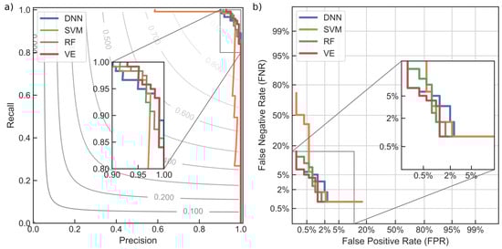
Figure 13.
Comparison of DNN, SVM, RF and VE classifiers: (a) receiver operating characteristic (ROC) curves presented on top of the isolines of constant –metric values; (b) detection error trade-off (DET) curves plotted in normal deviate scale.
In addition, Table 2 presents classifier comparisons in terms of different classification metrics obtained from the test set. Particularly notable is the comparison between classifiers in terms of the Jaccard and Matthews coefficients. It can be seen that the VE classifier increased both of these metric scores from those of the individual (SVM and RF) classifiers that went into the ensemble. It further had the highest recall among all classifiers, while retaining high precision, which was particularly important for the power system TSA problem. Finally, its Brier score was very low, which means that it was well calibrated.
Table 2.
Classification metrics of different classifiers measured on a test set.
Sensitivity Analysis and Discussion
Sensitivity of the classifiers to the increasing severity of the autoencoder’s dimensionality reduction (i.e., constriction of the bottleneck layer) has been analyzed as well. Aggregate results from several runs are reported, due to the stochastic nature of the encoding process. The resulting classifiers precision and recall (mean values) are provided in Figure 14 as bar graphs, for three different autoencoder’s coding dimensions of decreasing size. It can be seen that the classifiers performance decreased and volatility increased (“ticks” denote standard deviation) with the reduction in size of the coding dimensions. However, enough information was being preserved even with a severe dimensionality reduction, enabling the classifiers to retain a relatively high values of precision and recall.
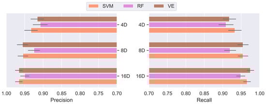
Figure 14.
Classifiers sensitivity to the increasing severity of the autoencoder’s dimensionality reduction.
Additionally, a further increase of the ensemble’s robustness could be achieved by introducing a pool of SVM estimators instead of using a single instance (i.e., by using the bootstrap aggregation of SVMs). A pool of SVM classifiers was first established by instantiating individual SVMs using stratified random subsamples from the training data set. Each model in the pool had different hyperparameters (obtained with the BO), and they competed with each other for dominance under the following constrained optimization:
where is the relative score of the j-th model and q is the number of models in the pool; y is a true class label and is a probability estimate of the unstable class. Optimization given by (17) essentially minimizes the cross-entropy of the pool of SVMs. A predicted probability, as a weighted average (based on their relative scores) from the entire pool of SVMs, was used in the final voting ensemble (Section 3.3). Table 3 presents optimal hyperparameters and relative scores for a pool of three SVMs. Introduction of this additional source of randomness and averaging into the model building process further decreased the ensemble’s variance and helped control the overfitting.
Table 3.
Hyperparameters and relative scores for a pool of SVM classifiers.
A combination of the undercomplete stacked autoencoder, which reduced the high-dimensionality of the original feature space (while preserving information), with a well-calibrated voting ensemble classifier, provided an overall well-balanced ML model for the power system TSA analysis. The high quality of the classification metrics, obtained from using a small number of input component features (i.e., codings), attested also to the performance of the autoencoder. Its full potential, however, would be revealed only on a much larger power system with many more signals/features [25]. A high performance of the SVM was confirmed, which partially stems from the use of Bayesian optimization for fine-tuning its hyperparameters. The ensemble, at the same time, pulled together predictions of two very different classifiers, building on their individual qualities in the process (in terms of robustness and classification performance).
Applying deep learning to the power system TSA problems will facilitate the next generation of TSA tools to move from preventive countermeasures (contingency analysis on pre-fault operating points) to corrective control. However, there are still important issues that need to be resolved. One such issue is the problem of transferability of deep learning models across different power systems. Namely, the principal downside of the end-to-end deep learning, which employs LSTM (and/or GRU) layers for ingesting raw time-series signals, is the inability to transfer learned information between different power system architectures [23]. Consequently, here proposed approach leverages expert knowledge for the features engineering (which is fully automated nonetheless). Another related issue concerns the computational resources needed for processing huge amounts of PMU signals using very complex deep learning models (that feature many millions of parameters). Further problems arise from the class imbalance of the data sets, noisy and missing data, labeling of cases for supervised learning, and other complexities of the real-world power systems.
5. Conclusions
A data-driven ML approach to solving the power system TSA was proposed in this paper. A novel 3.8 GB dataset of time-domain PMU–type signals was built from comprehensive electro–mechanical transient simulations of power system contingencies. It is openly shared under the CC-BY license. A sophisticate MATLAB/Simulink model of the IEEE New England 39-bus test case power system was built for that purpose and its flexibility greatly enhanced by the use of specialized blocks and object-oriented programming. A novel data processing pipeline was introduced for transforming the systematically generated dataset into the appropriate stochastic form (that captures class imbalance and statistical distribution of fault types), and splitting the data using the stratified shuffle approach. This dataset forms a convenient database for experimenting with different types of ML (including deep learning) models for the TSA analysis.
Furthermore, a complete ML based approach to the TSA classification has been proposed. It features an undercomplete denoising stacked autoencoder and a soft voting ensemble of SVM and RF base classifiers. Autoencoder, as an unsupervised learning model, can be trained (off-line) on a large corpus of unlabeled data. Its effectiveness in reducing/compressing the dimensionality of the feature space (without appreciable loss of information) has been corroborated in this case study. As a result, the training of the subsequent VE classifier is significantly faster and produces a better performing model at the same time. This effectiveness of the autoencoder is expected to increase with a larger data corpus. The classifier decisions can be used in real-time as inputs to the intelligent system for a corrective power system control and decision making. The voting ensemble pools (probabilistic) predictions from two very different base models and creates a weighted average that balances individual strengths of these underlying estimators. High performance of the VE classifier has been corroborated in this case study.
Applying deep learning to the power system TSA problems is showing promise, with several important issues that still need to be fully resolved. Training of complex deep learning architectures is still more of a black art than science, with special problems of convergence, vanishing gradients, forgetfulness, dead neurons, and others. A major issue is the problem of transferability of deep learning models across different power systems. In addition, many excellent deep learning architectures built, for example, for image processing can be applied in power system analysis only with great difficulties and uncertain performance in the real world. Building the next generation of TSA tools, using data mining and machine learning, is still a work in progress. This paper is seen as a contribution to the growing pool of knowledge and ML models that show great promise on standard benchmark test case power systems. However, stepping from benchmarks into the real world is often plagued with difficulties emanating from unforeseen circumstances. Therefore, future work will involve pursuing several avenues of research: (1) increasing the dataset size with new simulations, (2) increasing the class imbalance with new contingencies, (3) introducing different types of noise and measurement errors into the dataset for stress–testing the models, (4) using deep learning for features extraction from time-domain signals, (5) experimenting with engineering new artificial features and (6) testing different ensemble methods.
Supplementary Materials
The following are available online at https://www.zenodo.org/record/4521886.
Author Contributions
Conceptualization, P.S.; methodology, P.S. and A.K.; investigation, A.K. and M.D.; software, P.S. and A.K.; resources, G.P.; data curation, A.K.; writing—original draft preparation, P.S. and A.K.; writing—review and editing, G.P. and M.D.; visualization, P.S. and A.K.; project administration, G.P. All authors have read and agreed to the published version of the manuscript.
Funding
The work of A.K. has been fully supported by the “Young researchers’ career development project—training of doctoral students” of the Croatian Science Foundation, funded by the EU from the European Social Fund. This paper is fully supported by the Croatian Science Foundation under the project: “Power system disturbance simulator and non-sinusoidal voltages and currents calibrator” IP-2019-04-7292.
Institutional Review Board Statement
Not applicable.
Informed Consent Statement
Not applicable.
Data Availability Statement
The dataset is made available under the CC-BY license and deposited on Zenodo (contained within the Supplementary Materials section).
Conflicts of Interest
The authors declare no conflict of interest.
Abbreviations
The following abbreviations are used in this manuscript:
| ACC | Accuracy score |
| AF | Acquisition Function |
| ANN | Artificial Neural Network |
| AUC | Area Under Curve |
| AVR | Automatic Voltage Regulator |
| BO | Bayesian Optimization |
| BS | Brier score |
| DNN | Deep Neural Network |
| DET | Detection Error Trade-off |
| DT | Decision Tree |
| EAC | Equal Area Criterion |
| FNR | False Negative Rate |
| FPR | False Positive Rate |
| GRU | Gated Recurrent Unit |
| JC | Jaccard coefficient |
| LSTM | Long Short-Term Memory |
| MCC | Matthews correlation coefficient |
| ML | Machine Learning |
| PID | Proportional–Integral–Derivative |
| PMU | Phasor Measurement Unit |
| PPV | Positive Predictive Value |
| PSS | Power System Stabilizer |
| PV | Photovoltaic |
| RBF | Radial Basis Function |
| RF | Random Forest |
| ROC | Receiver Operating Characteristic |
| SVM | Support Vector Machine |
| TDS | Time-Domain Simulation |
| TL | Transmission Line |
| TPR | True Positive Rate |
| TSA | Transient Stability Assessment |
| TSI | Transient Stability Index |
| UCB | Upper Confidence Bound |
| VE | Voting Ensemble |
| WAMS | Wide Area Monitoring System |
References
- Zhang, Y.; Liu, W.; Wang, F.; Zhang, Y.; Li, Y. Reactive Power Control Method for Enhancing the Transient Stability Total Transfer Capability of Transmission Lines for a System with Large-Scale Renewable Energy Sources. Energies 2020, 13, 3154. [Google Scholar] [CrossRef]
- Alimi, O.A.; Ouahada, K.; Abu-Mahfouz, A.M. A Review of Machine Learning Approaches to Power System Security and Stability. IEEE Access 2020, 8, 113512–113531. [Google Scholar] [CrossRef]
- Perilla, A.; Papadakis, S.; Rueda Torres, J.L.; van der Meijden, M.; Palensky, P.; Gonzalez-Longatt, F. Transient Stability Performance of Power Systems with High Share of Wind Generators Equipped with Power-Angle Modulation Controllers or Fast Local Voltage Controllers. Energies 2020, 13, 4205. [Google Scholar] [CrossRef]
- Bruno, S.; De Carne, G.; La Scala, M. Distributed FACTS for Power System Transient Stability Control. Energies 2020, 13, 2901. [Google Scholar] [CrossRef]
- Wang, B.; Fang, B.; Wang, Y.; Liu, H.; Liu, Y. Power System Transient Stability Assessment Based on Big Data and the Core Vector Machine. IEEE Trans. Smart Grid 2016, 7, 2561–2570. [Google Scholar] [CrossRef]
- Wang, Y.; Chen, Q.; Hong, T.; Kang, C. Review of Smart Meter Data Analytics: Applications, Methodologies, and Challenges. IEEE Trans. Smart Grid 2019, 10, 3125–3148. [Google Scholar] [CrossRef]
- Sabo, A.; Wahab, N.I.A. Rotor Angle Transient Stability Methodologies of Power Systems: A Comparison. In Proceedings of the 2019 IEEE Student Conference on Research and Development, Bandar Seri Iskandar, Malaysia, 15–17 October 2019; pp. 1–6. [Google Scholar] [CrossRef]
- Pai, M.A. Energy Function Analysis for Power System Stability; Springer Science & Business Media: New York, NY, USA, 2012. [Google Scholar]
- Amraee, T.; Ranjbar, S. Transient instability prediction using decision tree technique. IEEE Trans. Power Syst. 2013, 28, 3028–3037. [Google Scholar] [CrossRef]
- Aghamohammadi, M.R.; Abedi, M. DT based intelligent predictor for out of step condition of generator by using PMU data. Int. J. Electr. Power Energy Syst. 2018, 99, 95–106. [Google Scholar] [CrossRef]
- Zhang, C.; Li, Y.; Yu, Z.; Tian, F. A weighted random forest approach to improve predictive performance for power system transient stability assessment. In Proceedings of the Asia-Pacific Power and Energy Engineering Conference APPEEC, Xi’an, China, 25–28 October 2016; pp. 1259–1263. [Google Scholar] [CrossRef]
- Baltas, N.G.; Mazidi, P.; Ma, J.; De Asis Fernandez, F.; Rodriguez, P. A comparative analysis of decision trees, support vector machines and artificial neural networks for on-line transient stability assessment. In Proceedings of the 2018 International Conference on Smart Energy Systems and Technologies, Seville, Spain, 10–12 September 2018; pp. 1–6. [Google Scholar] [CrossRef]
- Moulin, L.S.; Alves Da Silva, A.P.; El-Sharkawi, M.A.; Marks, R.J. Support vector machines for transient stability analysis of large-scale power systems. IEEE Trans. Power Syst. 2004, 19, 818–825. [Google Scholar] [CrossRef]
- Ye, S.; Li, X.; Wang, X.; Qian, Q. Power system transient stability assessment based on AdaBoost and support vector machines. In Proceedings of the Asia-Pacific Power and Energy Engineering Conference, Shanghai, China, 27–29 March 2012; pp. 1–4. [Google Scholar] [CrossRef]
- Hu, W.; Lu, Z.; Wu, S.; Zhang, W.; Dong, Y.; Yu, R.; Liu, B. Real-time transient stability assessment in power system based on improved SVM. J. Mod. Power Syst. Clean Energy 2019, 7, 26–37. [Google Scholar] [CrossRef]
- Mohammadi, M.; Gharehpetian, G.B. On-line transient stability assessment of large-scale power systems by using ball vector machines. Energy Convers. Manag. 2010, 51, 640–647. [Google Scholar] [CrossRef]
- Arefi, M.; Chowdhury, B. Ensemble adaptive neuro fuzzy support vector machine for prediction of transient stability. In Proceedings of the 2017 North American Power Symposium, Morgantown, WV, USA, 17–19 September 2017. [Google Scholar] [CrossRef]
- Karami, A.; Esmaili, S. Transient stability assessment of power systems described with detailed models using neural networks. Int. J. Electr. Power Energy Syst. 2013, 45, 279–292. [Google Scholar] [CrossRef]
- Hou, J.; Xie, C.; Wang, T.; Yu, Z.; Lü, Y.; Dai, H. Power system transient stability assessment based on voltage phasor and convolution neural network. In Proceedings of the 2nd IEEE International Conference on Energy Internet, Beijing, China, 21–25 May 2018; pp. 247–251. [Google Scholar] [CrossRef]
- Bahbah, A.G.; Girgis, A.A. New method for generators’ angles and angular velocities prediction for transient stability assessment of multimachine power systems using recurrent artificial neural network. IEEE Trans. Power Syst. 2004, 19, 1015–1022. [Google Scholar] [CrossRef]
- Yousefian, R.; Kamalasadan, S. A Review of Neural Network Based Machine Learning Approaches for Rotor Angle Stability Control. arXiv 2017, arXiv:1701.01214. [Google Scholar]
- Yu, J.J.; Hill, D.J.; Lam, A.Y.; Gu, J.; Li, V.O. Intelligent time-adaptive transient stability assessment system. IEEE Trans. Power Syst. 2018, 33, 1049–1058. [Google Scholar] [CrossRef]
- Azman, S.K.; Isbeih, Y.J.; Moursi, M.S.E.; Elbassioni, K. A Unified Online Deep Learning Prediction Model for Small Signal and Transient Stability. IEEE Trans. Power Syst. 2020, 35, 4585–4598. [Google Scholar] [CrossRef]
- Pan, F.; Li, J.; Tan, B.; Zeng, C.; Jiang, X.; Liu, L.; Yang, J. Stacked-GRU based power system transient stability assessment method. Algorithms 2018, 11, 121. [Google Scholar] [CrossRef]
- Zhu, Q.; Chen, J.; Zhu, L.; Shi, D.; Bai, X.; Duan, X.; Liu, Y. A Deep End-to-End Model for Transient Stability Assessment with PMU Data. IEEE Access 2018, 6, 65474–65487. [Google Scholar] [CrossRef]
- Zheng, L.; Hu, W.; Zhou, Y.; Min, Y.; Xu, X.; Wang, C.; Yu, R. Deep belief network based nonlinear representation learning for transient stability assessment. In Proceedings of the IEEE Power and Energy Society General Meeting, Chicago, IL, USA, 16–20 July 2017; pp. 1–5. [Google Scholar] [CrossRef]
- Yu, J.J.; Hill, D.J.; Lam, A.Y. Delay aware transient stability assessment with synchrophasor recovery and prediction framework. Neurocomputing 2018, 322, 187–194. [Google Scholar] [CrossRef]
- Zhu, L.; Hill, D.J.; Lu, C. Hierarchical Deep Learning Machine for Power System Online Transient Stability Prediction. IEEE Trans. Power Syst. 2020, 35, 2399–2411. [Google Scholar] [CrossRef]
- Tang, J.; Sui, H. Power System Transient Stability Assessment Based on Stacked Autoencoders and Support Vector Machine. IOP Conf. Ser. Mater. Sci. Eng. 2018, 452. [Google Scholar] [CrossRef]
- Azarbik, M.; Sarlak, M. Real-time transient stability assessment using stacked auto-encoders. COMPEL Int. J. Comput. Math. Electr. Electron. Eng. 2020, 39, 971–990. [Google Scholar] [CrossRef]
- Glorot, X.; Bengio, Y. Understanding the difficulty of training deep feedforward neural networks. J. Mach. Learn. Res. 2010, 9, 249–256. [Google Scholar]
- Bengio, Y. Deep Learning of Representations for Unsupervised and Transfer Learning. JMLR Workshop Conf. Proc. 2011, 7, 1–20. [Google Scholar]
- Murphy, K.P. Machine Learning: A Probabilistic Perspective, 4th ed.; MIT Press: Cambridge, MA, USA, 2013. [Google Scholar]
- Hang, F.; Huang, S.; Chen, Y.; Mei, S. Power system transient stability assessment based on dimension reduction and cost-sensitive ensemble learning. In Proceedings of the 2017 IEEE Conference on Energy Internet and Energy System Integration, Beijing, China, 26–28 November 2017; pp. 1–6. [Google Scholar] [CrossRef]
- Li, N.; Li, B.; Han, Y.; Gao, L. Dual cost-sensitivity factors-based power system transient stability assessment. IET Gener. Transm. Distrib. 2020, 14, 5858–5869. [Google Scholar] [CrossRef]
- Baltas, G.N.; Perales-González, C.; Mazidi, P.; Fernandez, F.; Rodríguez, P. A Novel Ensemble Approach for Solving the Transient Stability Classification Problem. In Proceedings of the 2018 7th International Conference on Renewable Energy Research and Applications (ICRERA), Paris, France, 14–17 October 2018; pp. 1282–1286. [Google Scholar] [CrossRef]
- Kunac, A.; Sarajcev, P. Ensemble Learning Approach to Power System Transient Stability Assessment. In Proceedings of the 2020 5th International Conference on Smart and Sustainable Technologies (SpliTech), Split, Croatia, 23–26 September 2020; pp. 1–6. [Google Scholar] [CrossRef]
- Liu, T.; Liu, Y.; Xu, L.; Liu, J.; Mitra, J.; Tian, Y. Non-parametric statistics-based predictor enabling online transient stability assessment. IET Gener. Transm. Distrib. 2018, 12, 5761–5769. [Google Scholar] [CrossRef]
- Li, X.; Zheng, Z.; Ma, Z.; Guo, P.; Shao, K.; Quan, S. Real-time approach for oscillatory stability assessment in large-scale power systems based on MRMR classifier. IET Gener. Transm. Distrib. 2019, 13, 4431–4442. [Google Scholar] [CrossRef]
- Kamari, N.A.M.; Musirin, I.; Othman, M.M. Application of evolutionary programming in the assessment of dynamic stability. In Proceedings of the 2010 4th International Power Engineering and Optimization Conference (PEOCO), Shah Alam, Malaysia, 23–24 June 2010; pp. 43–48. [Google Scholar] [CrossRef]
- MATLAB. Version 9.5 (R2018b); The MathWorks Inc.: Natick, MA, USA, 2018. [Google Scholar]
- Moeini, A.; Kamwa, I.; Brunelle, P.; Sybille, G. Open data IEEE test systems implemented in SimPowerSystems for education and research in power grid dynamics and control. In Proceedings of the Universities Power Engineering Conference, Stoke on Trent, UK, 1–4 September 2015; pp. 3–8. [Google Scholar] [CrossRef]
- Kundur, P. Power System Stability and Control; McGraw-Hill Inc.: New York, NY, USA, 1994. [Google Scholar]
- Zhou, Y.; Zhao, W.; Guo, Q.; Sun, H.; Hao, L. Transient Stability Assessment of Power Systems Using Cost-sensitive Deep Learning Approach. In Proceedings of the 2nd IEEE Conference on Energy Internet and Energy System Integration, Beijing, China, 20–22 October 2018; pp. 8–13. [Google Scholar] [CrossRef]
- Biswal, M.; Hao, Y.; Chen, P.; Brahma, S.; Cao, H.; De Leon, P. Signal features for classification of power system disturbances using PMU data. In Proceedings of the 19th Power Systems Computation Conference, Genoa, Italy, 20–24 June 2016; pp. 1–7. [Google Scholar] [CrossRef]
- Geeganage, J.; Annakkage, U.D.; Weekes, T.; Archer, B.A. Application of Energy-Based Power System Features for Dynamic Security Assessment. IEEE Trans. Power Syst. 2015, 30, 1957–1965. [Google Scholar] [CrossRef]
- Gurusinghe, D.R.; Rajapakse, A.D. Post-Disturbance Transient Stability Status Prediction Using Synchrophasor Measurements. IEEE Trans. Power Syst. 2016, 31, 3656–3664. [Google Scholar] [CrossRef]
- Géron, A. Hands-On Machine Learning with Scikit-Learn, Keras & TensorFlow, 2nd ed.; O’Reilly Media, Inc.: Sebastopol, CA, USA, 2019. [Google Scholar]
- Vincent, P.; Larochelle, H.; Lajoie, I.; Bengio, Y.; Manzagol, P.A. Stacked denoising autoencoders: Learning Useful Representations in a Deep Network with a Local Denoising Criterion. J. Mach. Learn. Res. 2010, 11, 3371–3408. [Google Scholar]
- Chollet, F. Deep Learning with Python, 1st ed.; Manning Publications Co.: Shelter Island, NY, USA, 2018. [Google Scholar]
- Abadi, M.; Agarwal, A.; Barham, P.; Brevdo, E.; Chen, Z.; Citro, C.; Corrado, G.S.; Davis, A.; Dean, J.; Devin, M.; et al. TensorFlow: Large-Scale Machine Learning on Heterogeneous Systems. 2015. Available online: https://www.tensorflow.org (accessed on 27 May 2021).
- Pedregosa, F.; Varoquaux, G.; Gramfort, A.; Michel, V.; Thirion, B.; Grisel, O.; Blondel, M.; Prettenhofer, P.; Weiss, R.; Dubourg, V.; et al. Scikit-learn: Machine Learning in Python. J. Mach. Learn. Res. 2011, 12, 2825–2830. [Google Scholar]
- Virtanen, P.; Gommers, R.; Oliphant, T.E.; Haberland, M.; Reddy, T.; Cournapeau, D.; Burovski, E.; Peterson, P.; Weckesser, W.; Bright, J.; et al. SciPy 1.0: Fundamental Algorithms for Scientific Computing in Python. Nat. Methods 2020, 17, 261–272. [Google Scholar] [CrossRef] [PubMed]
- Brochu, E.; Cora, V.M.; Freitas, N.D. A Tutorial on Bayesian Optimization of Expensive Cost Functions, with Application to Active User Modeling and Hierarchical Reinforcement Learning. arXiv 2010, arXiv:1012.2599v1. [Google Scholar]
- Snoek, J.; Larochelle, H.; Adams, R.P. Practical Bayesian optimization of machine learning algorithms. Adv. Neural Inf. Process. Syst. 2012, 4, 2951–2959. [Google Scholar]
- Li, L.; Jamieson, K.; DeSalvo, G.; Rostamizadeh, A.; Talwalkar, A. Hyperband: A Novel Bandit-Based Approach to Hyperparameter Optimization. arXiv 2018, arXiv:1603.06560. [Google Scholar]


Publisher’s Note: MDPI stays neutral with regard to jurisdictional claims in published maps and institutional affiliations. |
© 2021 by the authors. Licensee MDPI, Basel, Switzerland. This article is an open access article distributed under the terms and conditions of the Creative Commons Attribution (CC BY) license (https://creativecommons.org/licenses/by/4.0/).