Article

Three-Dimensional Unsteady Aerodynamic Analysis of a Rigid-Framed Delta Kite Applied to Airborne Wind Energy

by
Iván Castro-Fernández
1,
Ricardo Borobia-Moreno
2,
Rauno Cavallaro
1 and
Gonzalo Sánchez-Arriaga
1,*
1
Departamento de Bioingeniería e Ingeniería Aeroespacial, Universidad Carlos III de Madrid, Leganés, 28911 Madrid, Spain
2
Centro de Experimentación de “El Arenosillo” (CEDEA), Instituto Nacional de Técnica Aeroespacial, Mazagón, 21130 Huelva, Spain
*
Author to whom correspondence should be addressed.
Energies 2021, 14(23), 8080; https://doi.org/10.3390/en14238080
Submission received: 30 October 2021 / Revised: 27 November 2021 / Accepted: 30 November 2021 / Published: 2 December 2021
(This article belongs to the Special Issue Airborne Wind Energy Systems)

Abstract

:
The validity of using a low-computational-cost model for the aerodynamic characterization of Airborne Wind Energy Systems was studied by benchmarking a three-dimensional Unsteady Panel Method (UnPaM) with experimental data from a flight test campaign of a two-line Rigid-Framed Delta kite. The latter, and a subsequent analysis of the experimental data, provided the evolution of the tether tensions, the full kinematic state of the kite (aerodynamic velocity and angular velocity vectors, among others), and its aerodynamic coefficients. The history of the kinematic state was used as input for UnPaM that provided a set of theoretical aerodynamic coefficients. Disparate conclusions were found when comparing the experimental and theoretical aerodynamic coefficients. For a wide range of angles of attack and sideslip angles, the agreement in the lift and lateral force coefficients was good and moderate, respectively, considering UnPaM is a potential flow tool. As expected, UnPaM predicts a much lower drag because it ignores viscous effects. The comparison of the aerodynamic torque coefficients is more delicate due to uncertainties on the experimental data. Besides fully non-stationary simulations, the lift coefficient was also studied with UnPaM by assuming quasi-steady and steady conditions. It was found that for a typical figure-of-eight trajectory there are no significant differences between unsteady and quasi-steady approaches allowing for fast simulations.

1. Introduction

Airborne Wind Energy (AWE) systems constitute a relatively recent technology to harvest energy and produce traction from high-altitude winds. Important technological and theoretical progress led to the introduction of some prototypes in a pre-commercial phase [1]. Being AWE systems operated airborne, with an aircraft linked to the ground by a tether, aerodynamics is one of its critical areas. Whether the generation happens on the ground (ground generation) or onboard the aircraft (fly generation), a good aerodynamic characterization is important for the design, control, and optimization of these systems. For this reason, AWE community dedicated an important effort to develop aerodynamic models for particular AWE machines [2,3,4,5,6,7,8] and also to prepare numerical tools and experimental setups to study the plethora of AWE aircraft, which includes different types of kites and rigid-wings [9,10,11,12].
Due to their importance for AWE applications, previous numerical works on aerodynamics and aeroelasticity were mainly focused on Leading Edge Inflatable (LEI) and ram-air kites. Computational cost and model fidelity were the main drivers on the selection of the numerical methods. For instance, low-cost models such as a quasi-steady multiple-wake Vortex Lattice Method (VLM) have been applied to LEI kites and highlighted the importance of the position of the separation points of the flow [13]. Aeroelastic analysis on LEI and ram-air kites [14,15] also used a quasi-steady 3-dimensional VLM that allows modifications of the boundary conditions to include non-linear airfoil aerodynamic data from external databases [16]. Reduced order modeling techniques for the aerostructural optimization of morphing wings for AWE applications also used 3D steady VLM [17,18]. Steady Reynolds-Averaged Navier–Stokes (RANS) simulations were also used to study LEI kites in 2D [19] and 3D [6], and fluid structure interaction problems in 2D [20,21]. A 2D interactive boundary-layer approach was also proposed for a ram-air kite [22]. To the best of the author’s knowledge, no previous works on 3D unsteady potential aerodynamics applied to RFD kites exist in the literature.
Concurrently with the numerical work, experimental setups have also been developed to acquire real flight data and find from them the aerodynamic characteristics of the kites. Pioneer works on sensor fusion and estimation were mostly targeted to kite control [23,24] and used onboard Global Navigation Satellite System (GNSS) receivers, line angle sensors, cameras, inertial measurement units (IMU), and magnetometers, among others. The aerodynamic efficiency and the lift coefficient as a function of the ratio between power and steering lines were obtained for LEI and ram-air kites [25]. However, obtaining a full and reliable aerodynamic model requires the direct measurement of the aerodynamic velocity vector, i.e., its modulus, and the angle of attack and sideslip angle of the kite. For this reason, vanes attached to the bridle of the kite were incorporated to the test bench and helped to uncover the importance of the aerodynamic loading on the aerodynamic characteristics due to the kite deformation [26]. Estimation Before Modeling Techniques, a method largely used in the aerospace industry [27], was also proposed to obtain the aerodynamic model of LEI and Rigid-Framed Delta (RFD) kites in a systematic manner [28]. The authors proposed an Extended Kalman Filter for AWE systems that incorporates the aerodynamic force and torque into the state vector [29] and added to the experimental setup a multihole pitot tube for the in situ and accurate measurement of the full aerodynamic velocity vector. Key aerodynamic coefficients versus the angle of attack and the sideslip angle for the RFD kite studied in this work were obtained from the flight data acquired during multiple figure-of-eight trajectories [28].
Among the multiple applications of such an experimental aerodynamic model of the RFD kite, we focus here on the exploration of the validity of using numerical methods with a low computational cost on the aerodynamic modeling of AWE systems. This is a critical aspect for AWE flight simulators that have been specifically designed to remove the fast longitudinal oscillation of the tether to keep low the computational cost (see for instance [30] and references therein). The coupling of these flight simulators with broad databases of aerodynamic coefficients generated with numerical methods or directly with low-cost numerical codes is a key application in AWE. In this work, an in-house 3D and unsteady VLM within the UnPaM suite [31,32] has been adapted and used to predict the aerodynamic forces in the same flight conditions tested in ref. [28], and results have been compared. Such a combination of data helps in the validation of fast aerodynamic tools such as UnPaM and also provides interesting insights into the underlying aerodynamic phenomena. Moreover, unsteady effects, commonly ignored in previous numerical analyses in AWE systems, are here taken into account (within the assumption of potential flow) and assessed by means of comparison between steady, quasi-steady and unsteady modeling. Another novelty of the work is that the numerical analysis has been carried out using as kinematic input the experimental data of a maneuver that is relevant for AWE applications. The remainder of this article is organized as follows. Section 2 describes the methodology and tools used in this work. The comparison between the theoretical and the experimental aerodynamic models and the role of the unsteady effects are discussed in Section 3 and Section 4, respectively. Section 5 presents the conclusions of the work, its limits, and suggests some future works that can contribute to further effectively model RFD kite aerodynamics.

2. Methodology

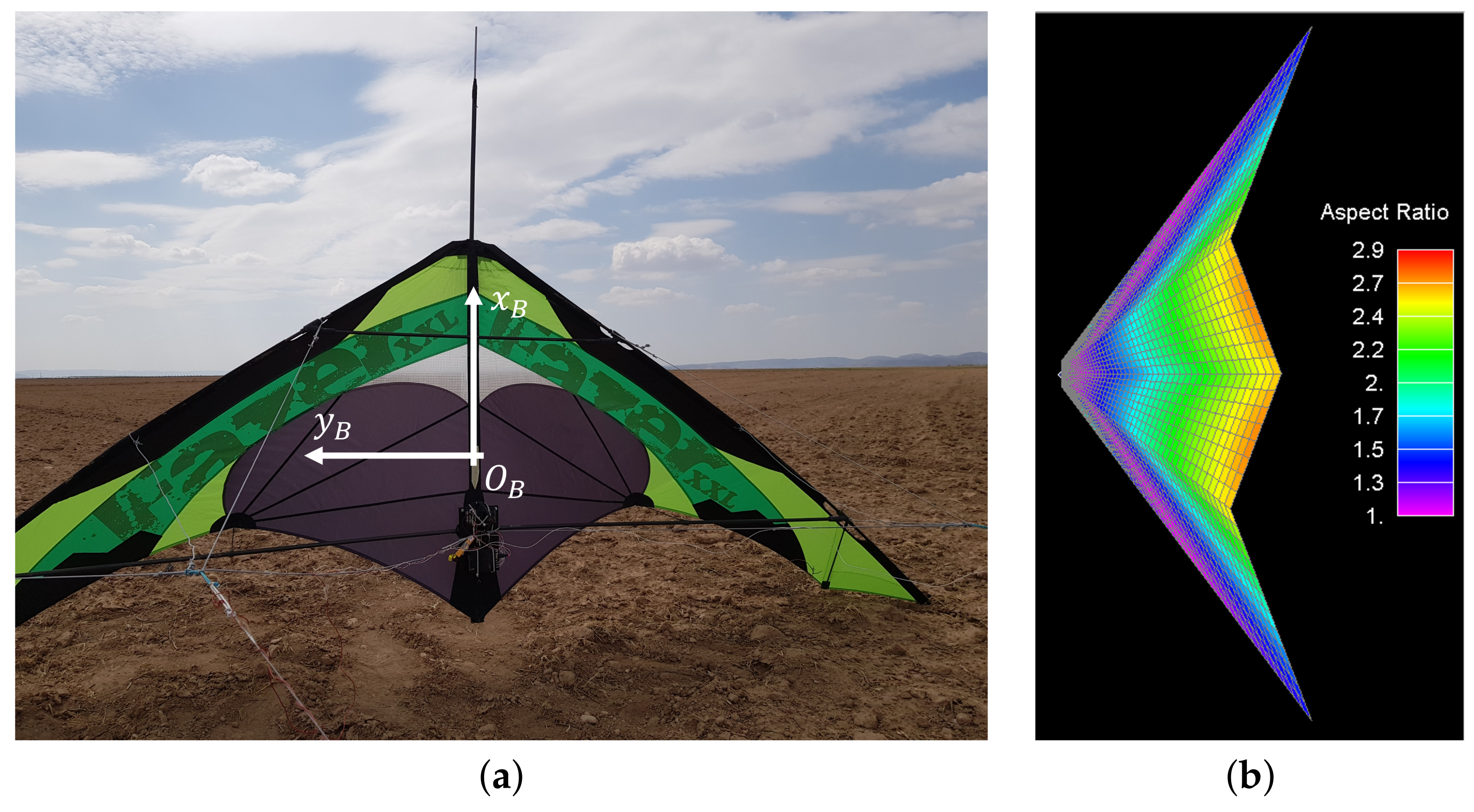
2.1. Flight Test Campaign

A previous work on an experimental AWE system [28] studied both LEI and RFD kites aerodynamics. The present work focuses on the same RFD kite (see Figure 1) and uses the experimental-based data obtained in ref. [28] through the Estimation Before Modeling technique. The reconstructed state vector of the kite along the crosswind trajectories included the kite position, ground speed, aerodynamic velocity vector, Euler angles, angular rates, and aerodynamic forces and moments. The experimental setup consisted of: (1) the two-line RFD kite equipped with onboard sensors: IMU, GNSS and an Aeroprobe TM micro Air Data System V2.0 composed of an onboard computer and a multi-hole pitot tube that was responsible for measuring the kite True AirSpeed ( T A S ), Angle of Attack ( α ), and SideSlip Angle ( β ); (2) a ground station for wind direction and magnitude measurements; and (3) load cells placed at each line of the kite to directly measure the tether tensions. The latter three sets of measurements constitute the observation model that, together with the process equation, constitute the discrete and continuous parts of the filter, respectively (more details are provided in refs. [28,29]).
Table 1 shows the physical characteristics of the RFD kite. The numerical tool explained in Section 2.2 was fed with these data in order to assess the performances of the kite. Properties I x B , I y B and I z B represent the principal moments of inertia about the kite Center of Mass (CM). For convenience, we define the body axes with origin at the CM, x B -axis along the spine of the kite, z B -axis normal to it and contained in the plane of symmetry of the kite (pointing towards the anchoring point in normal flight conditions) and y B -axis completing the right-handed frame. The body axes coincide with the principal axes of inertia. The chord (c) is defined as the mean aerodynamic chord of the RFD kite. The lines of the bridle meet at two points named A ± . Their coordinates in the body frame are x A ± , y A ± and z A ± . These last data have been revised by direct measurement with respect to the previous work [28]. Additionally, tether length, total frontal area of the two tethers and typical values for the tether drag coefficient from refs. [33,34] are provided.
The trajectory selected in this work is a figure-of-eight. Using the methodology of ref. [28], the temporal evolution of any variable of interest versus time throughout this trajectory can be obtained, including the true aerodynamic speed, the tether tensions, the angle of attack, the sideslip angle, Euler angles, aerodynamic coefficients, etc. For instance, Figure 2a,b show the orbit followed by the center of mass of the kite in one of these trajectories during the experimental campaign. The color corresponds to the magnitudes of the experimental true airspeed and the total tether tension (sum of the two tether tensions). For convenience, we used the Earth-fixed frame, that has origin at the anchoring point of the kite, x E -axis and y E -axis pointing toward the geographic north and east, respectively, and z E -axis pointing downwards. As expected, the maximum aerodynamic velocities and tether tension are reached in the straight legs of the trajectory where, as shown in Figure 2c, the angle of attack reaches a minimum. The side slip angle (Figure 2d) changes its sign several times during the orbit and it is mainly an anti-symmetric function with respect to the plane of symmetry of the figure-of-eight. There is a good confidence about the quality of the estimation of these four magnitudes ( T A S , tension, α , and β ) because all of them are directly measured by the multi-hole pitot tube and the load cells, and their measurements were introduced in the observation model.

2.2. In-House Three-Dimensional Unsteady Panel Method (UnPaM)

UnPaM [31,32] is a code capable of carrying out 3D aerodynamic simulations by using approaches based on the boundary element method. The flow field properties are described by singularities placed on the aerodynamic surface of the object and whose intensities are computed by imposing the boundary conditions. For incompressible flows, effects of unsteadiness concern the time-evolution of the circulation released in the wake and the time-dependent contribution in the momentum (Bernoulli’s) equation (find more details in Section 2.2.3). For a correct modeling of the wake, its evolution must be tracked, which typically leads to the so-called 3D wake roll-up.
UnPaM can handle thick and thin (zero-thickness) aerodynamic surfaces. For thin surfaces, considered hereafter due to its inherent suitability to model the flat canopy of the RFD kite, the method becomes the VLM. This makes use of quadrilateral constant-strength vortex rings lying on the panel boundaries/segments. The collocation points, i.e., nodes where the boundary conditions must be fulfilled, are located at the panel centers. The boundary element method imposes the well-known boundary condition for an impenetrable boundary,
v i + V i · n i = 0 , ( i = 1 N b ) ,
where v i is the perturbation velocity vector induced by all the panels, including also wake panels, on the body panels. Vectors V i and n i are the external velocity vector, i.e., the local velocity of the air with respect to the kite, and normal vector to the panel at the collocation point i, which runs from 1 to the total number of body panels N b . Since the perturbation velocity can be expressed as a superposition of the velocities induced by all the panels (body and wake), Equation (1) becomes a system of N b linear algebraic equations with N b unknowns that are the bound circulation strengths. When they are all gathered in the vector Γ , Equation (1) reads
A ¯ Γ = B ¯ Γ w C ,
with A ¯ and B ¯ the aerodynamic influence coefficient matrices of the body and wake panels on the body collocation points (further details in ref. [32]) and the N b components of vector C given by C i = V i · n i .
The wake is shed from the Trailing Edge (TE) and grows in length as the simulation time-stepping advances. In our non-stationary computations, the wake grows until it reaches a maximum dimension defined a priori in the simulation setup. Afterwards, the oldest wake panels are not modeled any more. For a generic time step, the new wake row in the computational domain and shed by the TE has circulation intensity determined by the Kutta condition:
Γ T E w = Γ TE ,
with subscripts T E standing for Trailing Edge panels and superscript w indicating the first row of wake panels, i.e., the one immediately after the kite. This equation enforces no circulation on the TE and, consequently, no flow around the TE by just equating intensities of panels sharing the TE segments. The wake panels that have been shed previously retain the same circulation intensities. Along the time-stepping procedure, every wake panel will move in accordance with its corner points. Therefore, every corner point is displaced by multiplying the velocity induced by both the external conditions and the singularities over the body and wake by the simulation time step. To initialize the wake in the computational model used in this work, 10 time steps are carried out with the kite at constant speed with no rotations. For further details of UnPaM’s algorithm, a self-explanatory high-level flowchart of UnPaM is presented in Appendix A.

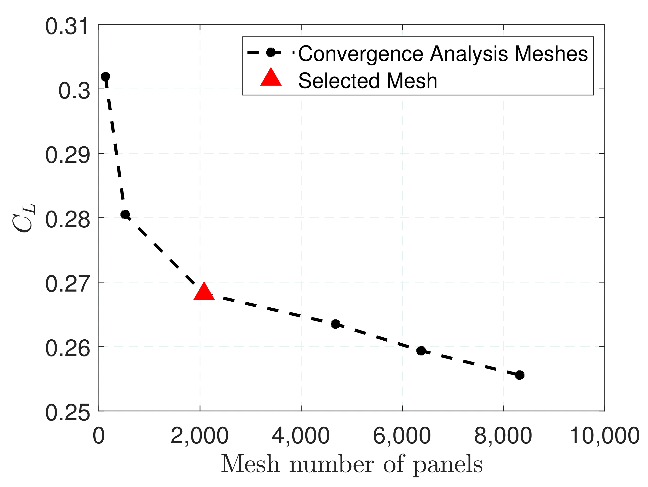
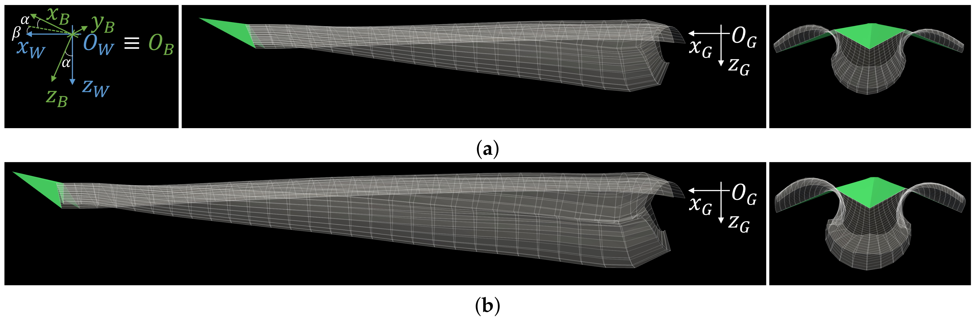
2.2.1. Aerodynamic Mesh

The VLM requires a lattice-like mesh composed of flat panels (see Figure 1). The kite geometry was split into four surfaces, two of them on each side of the symmetry plane. Each of these surfaces was discretized using quadrilateral elements. To guarantee a high-quality mesh, the elements aspect ratio, i.e., the fraction between the sides of the panel was bounded below 3. Consequently, and since the four surfaces become tapered toward the Leading Edge (LE), a graded mesh was obtained. Figure 3 shows a convergence analysis by varying the number of panels and monitoring relevant aerodynamic outputs of the tool, such as the lift coefficient for steady conditions at α = 20 and β = 0 . Hereafter, we consider a mesh with 2080 panels because, as shown in Figure 3, it has a good balance between computational cost and accuracy. Its error for the C L is less than 5% as compared with the finest mesh considered in Figure 3. For the selected mesh, the computational time for one time step in an unsteady simulation is in the order of a second.
The correct implementation of the method was verified by considering a flat delta wing with an aspect ratio similar to the one of the RFD kite and comparing the results with previous works. Delta wing aerodynamic characteristics have long been of interest to the aerospace industry [35,36,37,38] and it is well-known that they develop leading edge vortices for low enough aspect ratio at high angles of attack. Among them, we verified that UnPaM was able to reproduce the lift coefficient versus angle of attack curve of ref. [35] and the aspect ratio of our RFD kite is not low enough to generate important leading edge vortices.

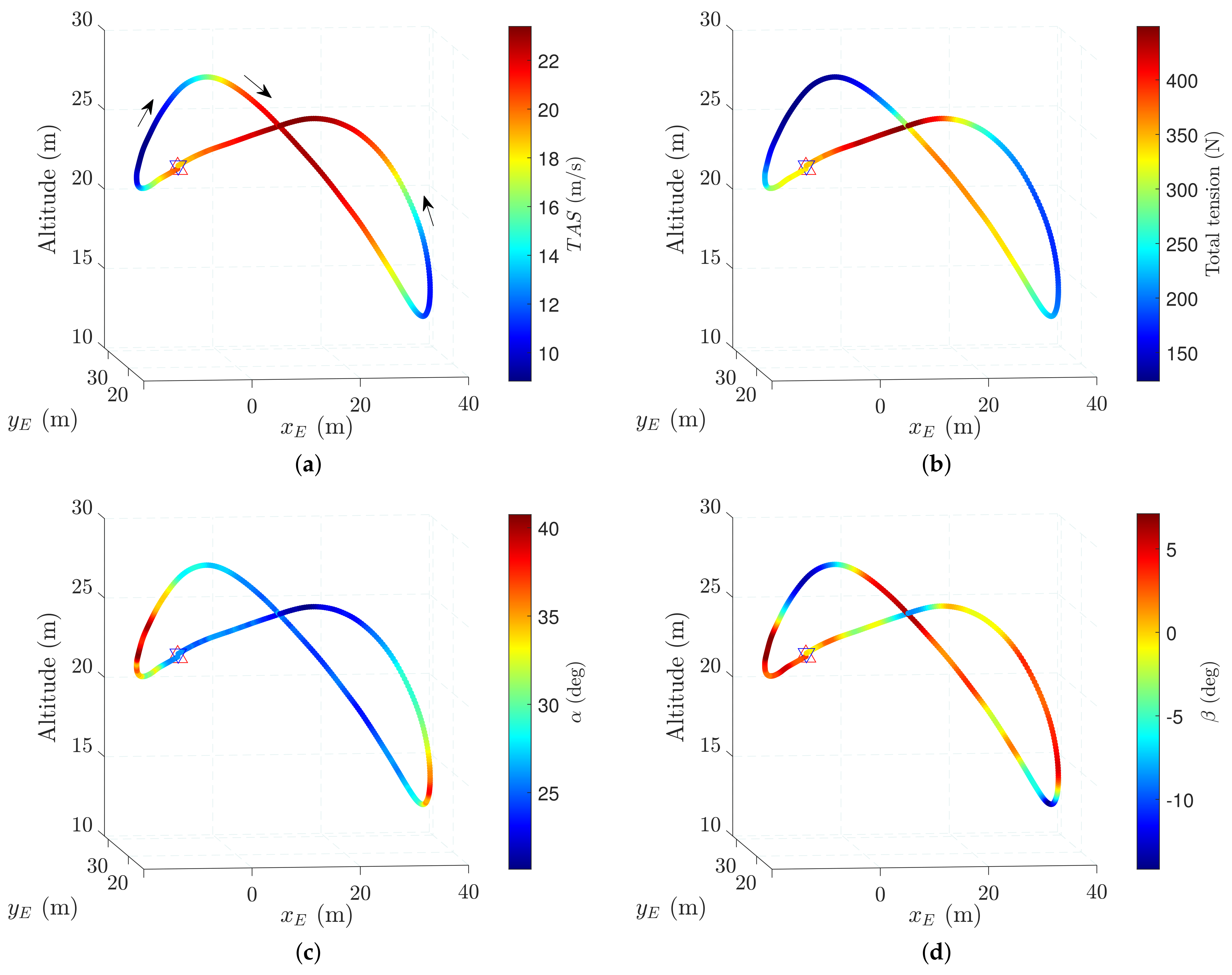
2.2.2. Kinematic Module of UnPaM

UnPaM has a module that is used to prescribe any relative motion between the kite and the fluid. This module is purely kinematic and not dynamic, i.e., aerodynamic loads are computed as the result of the motion defined by the user. The two relevant frames of reference in the simulations are the wind (identified by index W) and the body (identified by index B) frames, both of them with origin at the center of mass of the kite. The former has the x W -axis along the aerodynamic velocity vector whereas the z W -axis lies on the plane of symmetry of the kite and points towards the ground in normal flight conditions. Axis y w completes the right-handed frame. For convenience, we introduce a third frame, called the global frame (identified by index G), that has axes parallel to the wind frame and is at rest with respect to the computational box, i.e., everything else moves with respect to this frame. Therefore, the origin of the wind and the body frames move at the T A S along the x G -axis.
The inputs of the kinematic module, which fully define the motion of the kite with respect to the fluid, are the true aerodynamic speed, the angle of attack, the sideslip angle, and their time derivatives ( α ˙ , β ˙ ). All these quantities were mainly estimated by using the information of the multi-hole pitot tube onboard the kite in the experiments [28]. In fact, this is one of the main advantages of this kinematic arrangement in the numerical simulations because it is mainly based on the measurements of the multihole pitot tube, which is a high accuracy instrument. The position of the center of mass of the kite are found from them by solving the kinematic relation
d O G O B ¯ d t = T A S i G ,
with the initial condition O G O B ¯ = 0 . The attitude of the kite with respect to the fluid is given by the rotation matrix R ¯ W B that relates vector components in the wind and the body frames
i W j W k W = R ¯ WB i B j B k B cos α cos β sin β sin α cos β cos α sin β cos β sin α sin β sin α 0 cos α i B j B k B
and the angular velocity of the kite with respect to the fluid is
ω BG = ω BW = β ˙ sin α i B + α ˙ j B + β ˙ cos α k B .
Figure 4 displays the kite and the wake at two different instants of a simulation. The three reference frames and the wake roll-up behind the kite are shown. Figure 4a corresponds to the 20th time step in the simulation, when the kite has α = 26.1 º and β = 2.7 º (definitions of α and β rotations in Figure 4a left). Figure 4b shows the 30th time step with α = 32.0 º and β = 5.4 º. Although the kite moves to the left, it never reaches an exit boundary because the computational box is infinitely long. However, the maximum size of wake is finite and prescribed by the user at the beginning of the simulation.

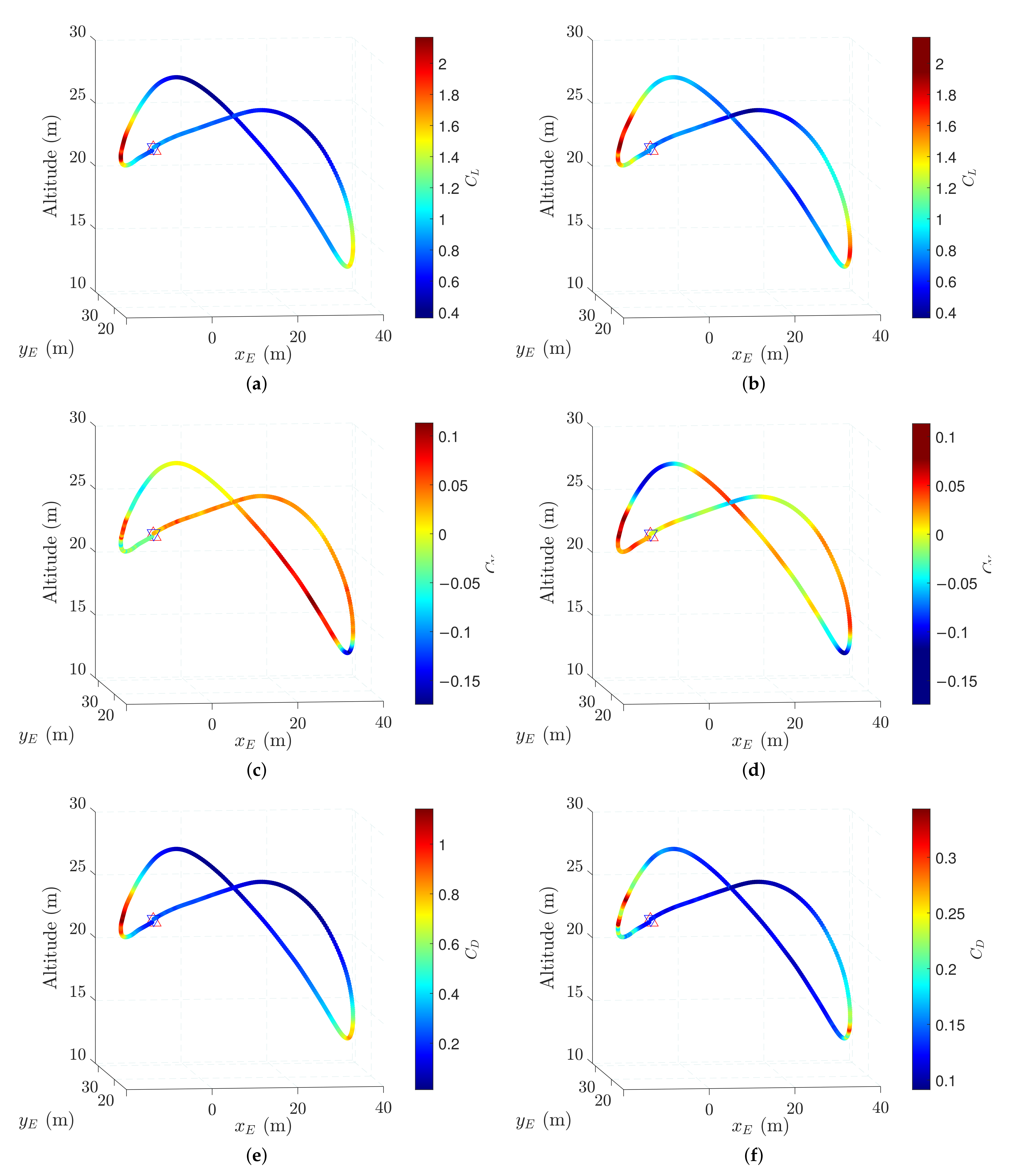
2.2.3. Force and Moment Coefficients Computation with UnPaM

UnPaM computes the aerodynamic forces by summing up the contributions of all the segments of the panels. For segment j of panel i, the Kutta–Joukowski theorem states,
f ij = ρ Γ i V ij × l ij , i = 1 N p , j = 1 , 4 ,
where ρ is the air density, Γ i the panel circulation, V ij the aerodynamic velocity vector at the center of the segment and vector l ij points in the direction of the segment circulation and has a magnitude equal to the segment length. The force acting on each panel ( f i ) is found from
f i = j = 1 4 f ij + ρ S i Γ i k Γ i k 1 Δ t n i , i = 1 N p ,
where S i and n i are the panel area and the unit vector normal to the panel, respectively. Superscripts k and k 1 stand for actual and previous time steps, whereas Δ t is the time step, which was kept constant during the simulation. The first and second term in Equation (8) correspond to the steady (or quasi-steady) and unsteady force components. The latter, which corresponds to a backward finite difference approximation of the time derivative, takes into account the temporal change of the panel circulation. The panel contribution to the total aerodynamic moment about the center of mass of the kite is
m i = r i × f i , i = 1 N p ,
with r i a vector with origin at the center of mass of the kite and tip at the center of the panel. Coefficients for drag ( C D ), lateral ( C Y ) and lift ( C L ) forces together with those for roll ( C l ), pitch ( C m ) and yaw ( C n ) moments, which are the quantities used in this work to compare experimental and theoretical results, are obtained by summing for all the panels and normalizing in the standard manner
C D , C Y , C L = 2 ρ V 2 S i N p f i · i W , j W , k W ,
C l , C m , C n = 2 ρ V 2 S i N p m i · i B b , j B c , k B b .

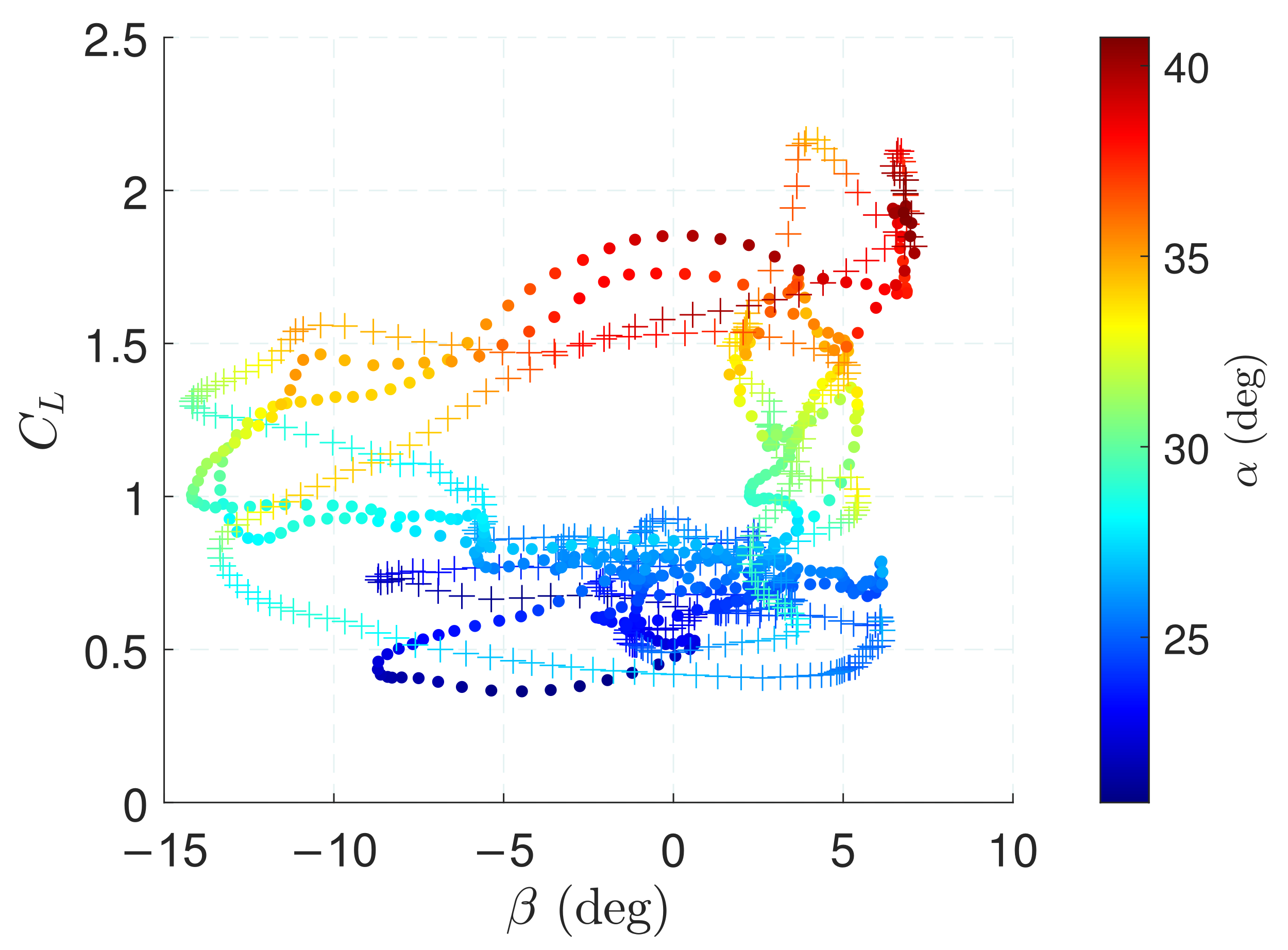
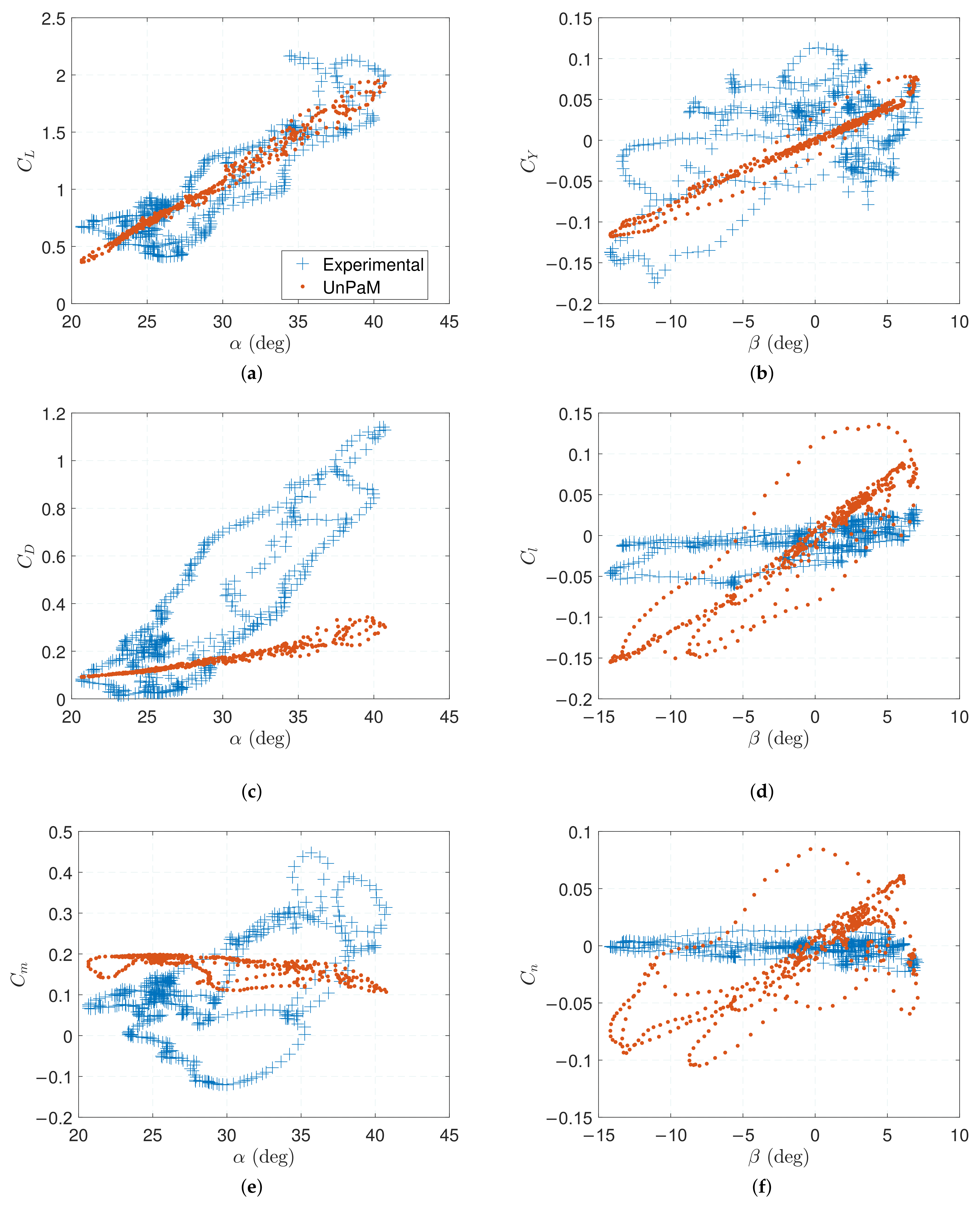
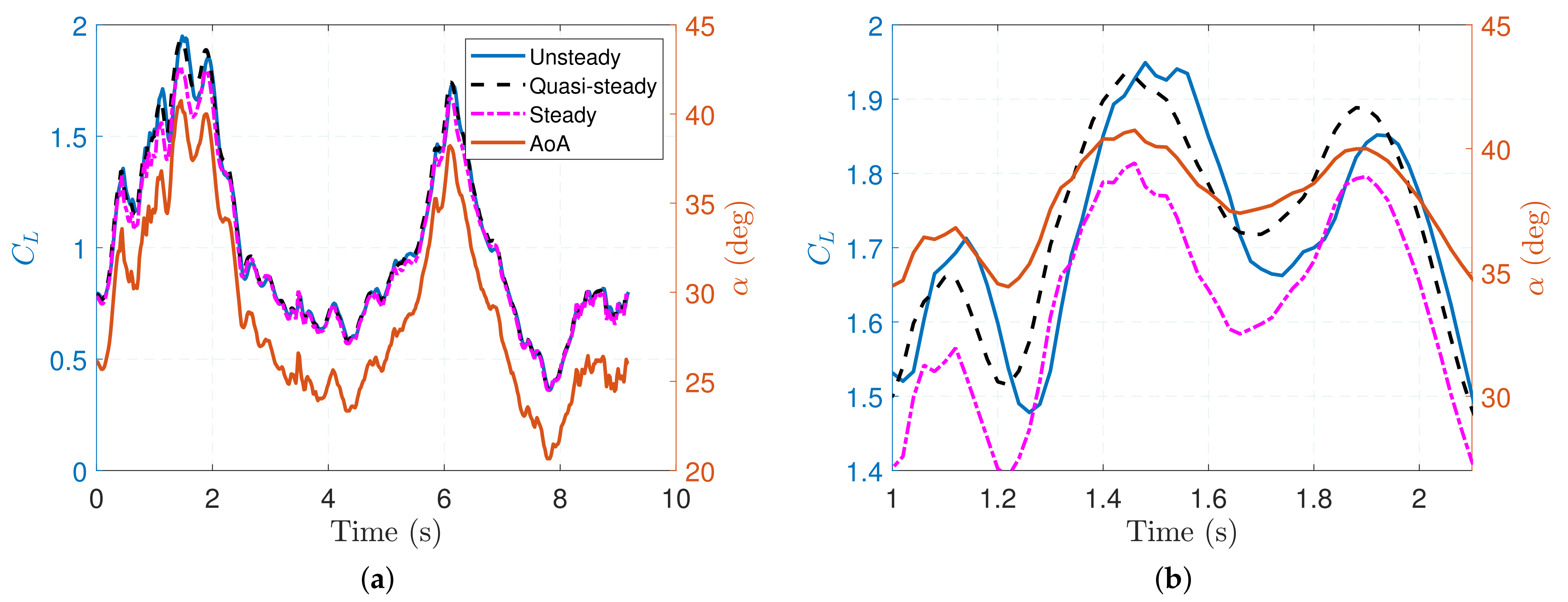
3. Comparison of Numerical and Experimental Results

This section compares the force and moment coefficients predicted by UnPaM and the one obtained by feeding the Extended Kalman Filter with the data measured in the experimental campaign [28]. The selected trajectory is the figure-of-eight shown in Figure 2. Figure 5 shows the six force and moment coefficients. Longitudinal ( C L , C D , and C m ) and lateral-directional ( C Y , C l , and C n ) coefficients are presented versus the angle of attack and the sideslip angle, respectively. Dots and crosses are used to show the results obtained from UnPaM and the experiments.
A good agreement was found for the lift coefficient C L (Figure 5a), resulting in an average error of around 20 % for the full trajectory. Interestingly, and although large values of the angle of attack are reached in the trajectory, the experimental results do not show the stall of the kite. Non-stationary effects have been suggested to explain this feature [28]. Such a circumstance may explain why UnPaM, which is a potential flow code with no flow separation, can reproduce reasonably well the experimental results for high angles of attack. It is also remarkable that the experimental C L versus α curve exhibits two values of the C L for the same angle of attack, whereas the dispersion of the values coming from the potential flow theory is very small. This is the main cause of mismatch (20%), however, numerical data is centered between the two possible experimental values for every α . Moreover, the dispersion of the experimental C L cannot be explained in terms of the different values of the sideslip angle reached by the kite in the trajectory, which also cover a small range (between 15 and 8 ). A confirmation that the angle of attack is the main driver of the C L is provided by Figure 6. It displays C L versus β and shows a moderate agreement for the trend between the experimental and the numerical results and an average error of around 20 % . This result reinforces the argument about the importance of non-stationary effects in RFD kites because there is hysteresis in the experimental C L α curve. Dynamic stall, which is a phenomenon that is not captured by the potential flow code, is a candidate to explain it.
The experimental drag coefficient shown in Figure 5c also exhibits hysteresis. For a fair comparison, the tether drag ( D t ) incorrectly attributed to the kite in ref. [28] has been subtracted from the total experimental drag following an overestimated approximation given in Equation (12). As expected, UnPaM, as a potential flow tool, captures relatively well the drag only for small angles of attack but, in general, the code underestimates C D . This mismatch is explained by the fact that UnPaM does not include viscous effects and flow separation. As a result, a large difference between the numerical and experimental drag results exist for large angles of attack. The lateral force coefficient in Figure 5b shows a moderate match in trend between the experimental and the numerical results. However, dispersion exhibited by the experimental C Y is not properly captured by the numerical tool probably due to span-wise complex separation phenomena. Interestingly, the figure-of-eight maneuver was carried out with a bias of around 5 in β , i.e., the range of β covered is not symmetric around β = 0 .
C D t = D t 1 / 2 ρ V 2 S = 1 / 2 ρ V 2 S t C d t 1 / 2 ρ V 2 S = S t S C d t .
Regarding the three moment coefficients, the magnitudes of the experimental and numerical results are in the same order, but there does not exist a clear match in trend between them. In this case, the comparison and the extraction of conclusions is more difficult. On the one hand, UnPaM has the limitations already discussed for the force coefficients, including the inability to capture flow separation. On the other hand, it is not clear that the procedure followed in ref. [28] can provide a high-accurate estimation of the aerodynamic moments. Unlike the T A S , the tension, the angle of attack, and the sideslip angle, the aerodynamic moments are not directly observed. Estimations of these magnitudes are provided by the Extended Kalman Filter by combining the process equations and the observation model. Moreover, the bridle of the kite was not considered in the state equations of the filter in ref. [28] and this impacts the estimations of C m , C L , and C n . Among them, the one with a better correlation between the experimental and the numerical results is C m .
Figure 7 shows the values of the force coefficients along the figure-of-eight trajectory. Experimental and numerical results are shown on the left and the right figures. To ease the comparison, the limits of the scale were set evenly for each pair of plots, except for the drag coefficient in Figure 7e,f. The general trend of the three force coefficients correlates reasonably well along the orbit. It also makes evident the very different conditions reached by the kite in the straight legs and the turning phases. The lift (Figure 7a,b) and drag (Figure 7e,f) coefficients reach their maxima in the turns where, eventually, the T A S (Figure 2) finds its minimum. The kite reduces its T A S in the turns, but its angle of attack increases to yield a high C L and C D . The opposite situation happens in the straight legs, where the T A S is large and the angle of attack and the force coefficients are small. This explains the high values of the tether tensions shown in Figure 2. The lateral force coefficient (Figure 7c,d) mainly follows the sideslip angle and it changes its sign along the trajectory.

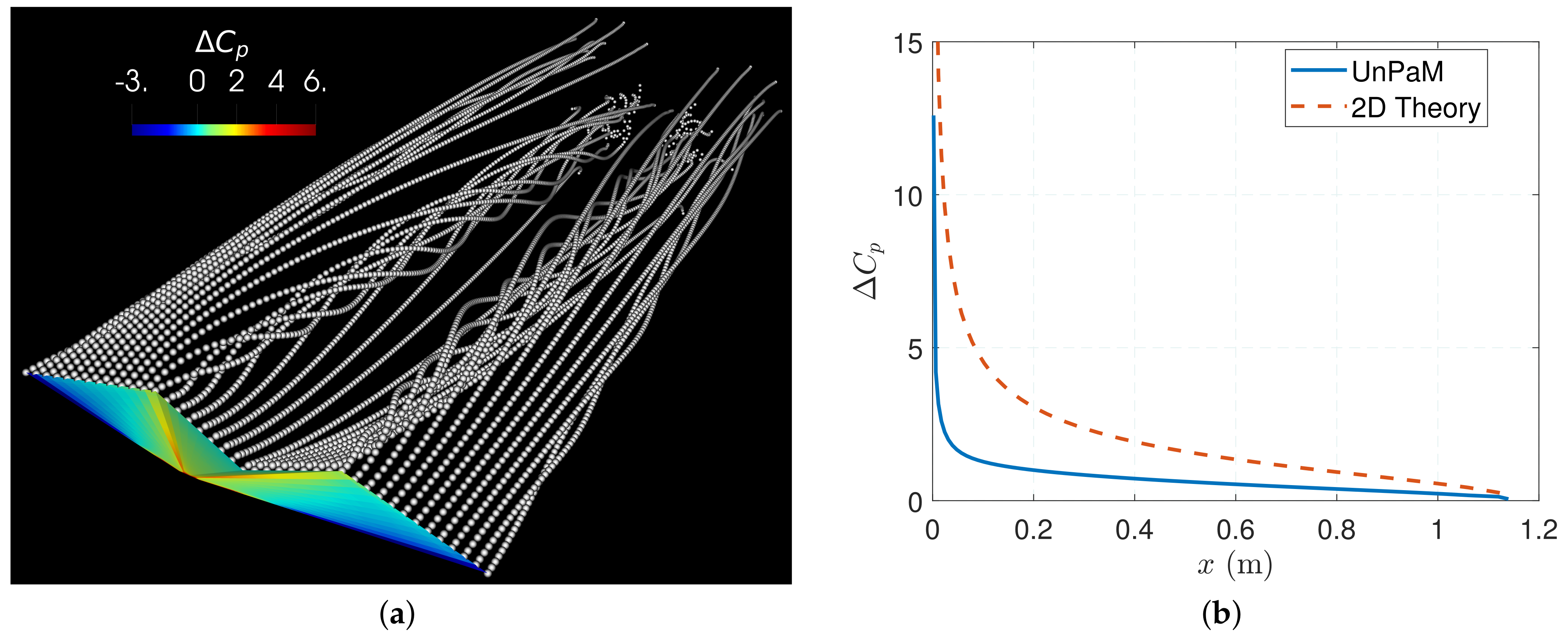
4. Analysis of the Potential Flow

Figure 8 shows the results of UnPaM for α = 20 , β = 0 and T A S = 10 m/s, which are the typical conditions found during the figure-of-eight maneuver. UnPaM, which is a potential flow code, may work properly for these conditions because we checked that the zero-lift line is at an angle of attack of 15 . As explained in Section 2.2.2, the angle of attack is measured with respect to the spine of the kite in our analysis. The color in Figure 8a indicates the difference of the pressure coefficient between the intrados and extrados ( Δ C p ). A very different behavior is observed at the two planes closer to the spine of the kite than in the two other planes that contain the leading edge because these two families of planes have a very different dihedral angle. Consequently, the coefficient Δ C p is positive in the inner part of the kite and negative at the leading edge for this specific angle of attack. The maximum Δ C p is reached at the two diagonals where the planes intersect. These 3-dimensional results have been compared with the Δ C p of a 2-dimensional flat plate. Figure 8b shows the distribution of Δ C p along the spine of the kite from UnPaM and Equation (13) of ref. [39] that reads
Δ C p = 4 c s x x α , x x C M x B ,
where c s = 1.16 m is the length of the spine of our RFD kite, x C M = 0.71 m is the distance between its nose and center of mass, and x B is the coordinate in the body frame. Due to three-dimensional effects, there is a mismatch between both curves and, as expected, UnPaM predicts a lower Δ C p . The simulation also provides valuable information about the structure of the wake. As shown in Figure 8a, two pairs of counter-rotating vortices are formed. The first pair starts at the tips of the kite and the second appears at the intersections of the two families of planes. Opposite roll-up is observed for the vortices generated at the tips and the intersections lines due to the different dihedral angles of the planes that produce Δ C p with different signs.
In order to obtain an idea of the unsteady effects in the flight of the RFD kite, we present now three different types of results: (i) unsteady results obtained by implementing the methodology explained in Section 2.2, (ii) quasi-steady results obtained such as in (i) but ignoring the second term in Equation (8) and eliminating the roll-up of the wake by forcing the geometry of its panels, and (iii) steady results obtained such as in (ii) but setting ω BW = 0 . Figure 9a shows the lift coefficient of the three approaches versus time (left axis) and, for convenience, it also displays the evolution of the angle of attack (right axis) in the figure-of-eight trajectory. The three approaches give the same results for the straight legs of the figure of eight, where the angle of attack and the angular velocity are small and the T A S is high. The main differences occur during the turns, as shown in the detail provided in Figure 9b. The steady approximation mostly underestimates the value of C L . Interestingly, there exists a lag between the C L and α in the unsteady approximation. The maxima of the C L in the unsteady approximation occurs later than the maxima of the angle of attack. Regarding the steady and the quasi-steady approximations, the maxima of the C L and the α curves occur simultaneously. Even during the turning, the differences are small and a steady or a quasi-steady simulation may suffice for the aerodynamic modeling of RFD kites flying in crosswind trajectories.

5. Conclusions

This work benchmarked a three-dimensional unsteady potential aerodynamic tool against experimental data obtained in a flight campaign with a rigid-framed delta kite of 1.86 m 2 . A figure-of-eight orbit, which is the relevant trajectory for airborne wind energy systems, was studied in detail. The kinematic state of the kite in the experiments was used as input for the code. A good and moderate agreement for the lift and the lateral force coefficients, respectively, was found. The drag coefficient matched only for low values of the angle of attack. The potential flow code underestimated the drag because ignores viscous effects. Theoretical and experimental moment coefficients are in the same order of magnitude but they do not follow the same trend. In this case, the confidence on the moment coefficients estimated in the experimental campaign is lower than in the case of the forces due to issues related to the modelization of the bridle of the kite and the comparison is troublesome. The experimental and theoretical results presented in this work are a step toward the understanding and characterization of kite aerodynamics, but more reliable data for the aerodynamic moments (experimental and theoretical) are still necessary.
The experimental results revealed that the lift and drag coefficients can take different values when presented as just a function of the angle of attack. The potential flow code, and a fine analysis of the experimental result, showed that this is not due to a possible dependence of C L on the sideslip angle. This hysteresis in the C L and C D versus α curves, and also the high values of lift coefficients measured in the experiments, may be a consequence of unsteady phenomena. Dynamic stall, which is experienced by wings subject to periodic pitching motions, is one of the candidates to explain it. The results of this study suggest that future works on including dynamic stall semi-empirical methods in the numerical codes can help improve the aerodynamic characterization of the RDF kite while keeping low its computational cost.
UnPaM’s performance in terms of computational time opens the possibility for coupling this tool with AWE flight simulators. In particular, if UnPaM is combined with AWE models based on inelastic tethers to remove the fast time scale (longitudinal waves along the tether), a low-computational-cost numerical tool can be prepared. For instance, for the aerodynamic mesh used in this work, the computational time for UnPaM to carry out one time step in our machine is in the order of magnitude of a second. Considering that the real time required by the kite to perform a full figure-of-eight trajectory is 10 s, and a time-step in the dynamic simulations can be in the order of 1 × 10 2 s, the total time to simulate a full orbit is less than half an hour. Moreover, this work demonstrated that a quasi-steady approximation within the UnPaM suite can be sufficient for the characterization of the lift coefficient during the figure-of-eight trajectory and this can be use to speed-up the simulations. Therefore, the tool could be used for broad parametric analysis and optimal control with medium fidelity. Real-time simulations would be also possible by using the code to generate a broad database of aerodynamic coefficients as a function of the angle of attack and the sideslip angles.

Author Contributions

Conceptualization, R.C. and G.S.-A.; Formal analysis, I.C.-F. and R.B.-M.; Methodology, I.C.-F. and R.B.-M.; Software, I.C.-F. and R.C.; Writing—original draft, I.C.-F.; Writing—review and editing, R.B.-M., R.C., and G.S.-A. All authors have read and agreed to the published version of the manuscript.

Funding

This work was carried out under the framework of the GreenKite-2 project (PID2019-110146RB-I00) funded by MCIN/AEI/10.13039/501100011033.

Institutional Review Board Statement

Not applicable.

Informed Consent Statement

Not applicable.

Conflicts of Interest

The authors declare no conflict of interest.

Abbreviations

The following abbreviations are used in this manuscript:
AWEAirborne Wind
CMKite Center of Mass
GNSSGlobal Navigation Satellite System
IMUInertial Measurement Unit
LELeading Edge
LEILeading Edge Inflatable
RANSReynolds-Averaged Navier-Stokes
RFDRigid-Framed Delta
TETrailing Edge
UnPaMUnsteady Panel Method
VLMVortex Lattice Method

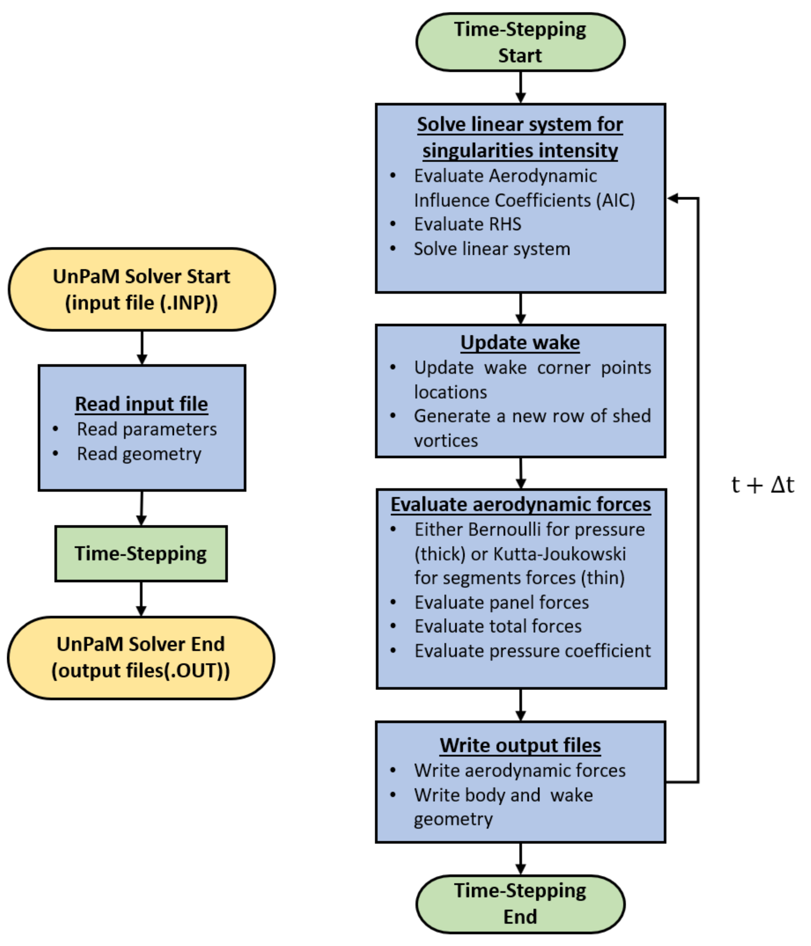
Appendix A. UnPaM High-Level Flowchart

Figure A1 shows a flowchart of the aerodynamic tool UnPaM. The unsteady simulations carried out in this tool are based on a time-stepping algorithm based on a Runge-Kutta 4 integrator to update the relevant kinematic variables (Section 2.2.2). At every time step, the kinematic variables are read and the potential flow is found by using the panel method explained in Section 2.2. The wake of the kite grows gradually until reaching a maximum size defined by the user at the beginning of the simulation. A full description of UnPaM is in [31,32].
Figure A1. High-level flowchart of UnPaM in unsteady simulations.
Energies 14 08080 g0a1

References

  1. European Commission. Study on Challenges in the Commercialisation of Airborne Wind Energy Systems; Technical Report; EU Publications: Brussels, Belgium, 2018. [Google Scholar] [CrossRef]
  2. Vimalakanthan, K.; Caboni, M.; Schepers, G.; Pechenik, E.; Williams, P. Aerodynamic analysis of Ampyx’s airborne wind energy system. J. Phys. Conf. Ser. 2018, 1037, 062008. [Google Scholar] [CrossRef] [Green Version]
  3. Malz, E.; Koenemann, J.; Sieberling, S.; Gros, S. A reference model for airborne wind energy systems for optimization and control. Renew. Energy 2019, 140, 1004–1011. [Google Scholar] [CrossRef]
  4. Mehr, J.; Alvarez, E.J.; Ning, A. Unsteady aerodynamic analysis of wind harvesting aircraft. Aiaa Aviat. 2020 Forum 2020, 1, 1–13. [Google Scholar] [CrossRef]
  5. Wijnja, J.; Schmehl, R.; De Breuker, R.; Jensen, K.; Lind, D.V. Aeroelastic analysis of a large airborne wind turbine. J. Guid. Control. Dyn. 2018, 41, 2374–2385. [Google Scholar] [CrossRef]
  6. Viré, A.; Demkowicz, P.; Folkersma, M.; Roullier, A.; Schmehl, R. Reynolds-averaged Navier-Stokes simulations of the flow past a leading edge inflatable wing for airborne wind energy applications. J. Phys. Conf. Ser. 2020, 1618. [Google Scholar] [CrossRef]
  7. Ali, Q.S.; Kim, M.H. Unsteady aerodynamic performance analysis of an airborne wind turbine under load varying conditions at high altitude. Energy Convers. Manag. 2020, 210, 112696. [Google Scholar] [CrossRef]
  8. Saleem, A.; Kim, M.H. Aerodynamic performance optimization of an airfoil-based airborne wind turbine using genetic algorithm. Energy 2020, 203, 117841. [Google Scholar] [CrossRef]
  9. Cherubini, A.; Papini, A.; Vertechy, R.; Fontana, M. Airborne Wind Energy Systems: A review of the technologies. Renew. Sustain. Energy Rev. 2015, 51, 1461–1476. [Google Scholar] [CrossRef] [Green Version]
  10. Vermillion, C.; Cobb, M.; Fagiano, L.; Leuthold, R.; Diehl, M.; Smith, R.S.; Wood, T.A.; Rapp, S.; Schmehl, R.; Olinger, D.; et al. Electricity in the air: Insights from two decades of advanced control research and experimental flight testing of airborne wind energy systems. Annu. Rev. Control. 2021. [Google Scholar] [CrossRef]
  11. Licitra, G.; Williams, P.; Gillis, J.; Ghandchi, S.; Sieberling, S.; Ruiterkamp, R.; Diehl, M. Aerodynamic Parameter Identification for an Airborne Wind Energy Pumping System. IFAC-PapersOnLine 2017, 50, 11951–11958. [Google Scholar] [CrossRef]
  12. Licitra, G.; Bürger, A.; Williams, P.; Ruiterkamp, R.; Diehl, M. Aerodynamic model identification of an autonomous aircraft for airborne wind energy. Optim. Control Appl. Methods 2019, 40, 422–447. [Google Scholar] [CrossRef]
  13. Leuthold, R. Multiple-Wake Vortex Lattice Method for Membrane-Wing Kites; Technical Report; Delft University of Technology: Delft, The Netherlands, 2015. [Google Scholar] [CrossRef]
  14. Candade, A.A.; Ranneberg, M.; Schmehl, R. Structural analysis and optimization of a tethered swept wing for airborne wind energy generation. Wind Energy 2020, 23, 1006–1025. [Google Scholar] [CrossRef]
  15. Candade, A.A.; Ranneberg, M.; Schmehl, R. Aero-structural Design of Composite Wings for Airborne Wind Energy Applications. J. Phys. Conf. Ser. 2020, 1618. [Google Scholar] [CrossRef]
  16. Ranneberg, M. Direct Wing Design and Inverse Airfoil Identification with the Nonlinear Weissinger Method. arXiv 2015, arXiv:1501.04983v2. [Google Scholar]
  17. Fasel, U.; Keidel, D.; Molinari, G.; Ermanni, P. Aerostructural optimization of a morphing wing for airborne wind energy applications. Smart Mater. Struct. 2017, 26, 095043. [Google Scholar] [CrossRef]
  18. Fasel, U.; Tiso, P.; Keidel, D.; Molinari, G.; Ermanni, P. Reduced-order dynamic model of a morphing airborne wind energy aircraft. AIAA J. 2019, 57, 3586–3598. [Google Scholar] [CrossRef]
  19. Folkersma, M.; Schmehl, R.; Viré, A. Boundary layer transition modeling on leading edge inflatable kite airfoils. Wind Energy 2019, 22, 908–921. [Google Scholar] [CrossRef] [PubMed]
  20. Bosch, A.; Schmehl, R.; Tiso, P.; Rixen, D. Dynamic nonlinear aeroelastic model of a kite for power generation. J. Guid. Control. Dyn. 2014, 37, 1426–1436. [Google Scholar] [CrossRef] [Green Version]
  21. Breukels, J.; Schmehl, R.; Ockels, W. Aeroelastic Simulation of Flexible Membrane Wings based on Multibody System Dynamics. In Airborne Wind Energy. Green Energy and Technology; Springer: Delft, The Netherlands, 2013; pp. 287–305. [Google Scholar] [CrossRef]
  22. Thedens, P.; de Oliveira, G.; Schmehl, R. Ram-air kite airfoil and reinforcements optimization for airborne wind energy applications. Wind Energy 2019, 22, 653–665. [Google Scholar] [CrossRef]
  23. Fagiano, L.; Huynh, K.; Bamieh, B.; Khammash, M. On Sensor Fusion for Airborne Wind Energy Systems. IEEE Trans. Control Syst. Technol. 2014, 22, 930–943. [Google Scholar] [CrossRef] [Green Version]
  24. Hesse, H.; Polzin, M.; Wood, T.A.; Smith, R.S. Visual motion tracking and sensor fusion for kite power systems. In Airborne Wind Energy. Green Energy Technology; Springer: Delft, The Netherlands, 2018; Volume 9789811019, pp. 413–438. [Google Scholar] [CrossRef]
  25. Hummel, J.; Göhlich, D.; Schmehl, R. Automatic measurement and characterization of the dynamic properties of tethered membrane wings. Wind Energy Sci. 2019, 4, 41–55. [Google Scholar] [CrossRef] [Green Version]
  26. Oehler, J.; Schmehl, R. Aerodynamic characterization of a soft kite by in situ flow measurement. Wind Energy Sci. 2019, 4, 1–21. [Google Scholar] [CrossRef] [Green Version]
  27. Hoff, J.; Cook, M. Aircraft parameter identification using an estimation-before-modelling technique. Aeronaut. J. 1968, 100, 259–268. [Google Scholar]
  28. Borobia-Moreno, R.; Ramiro-Rebollo, D.; Schmehl, R.; Sánchez-Arriaga, G. Identification of kite aerodynamic characteristics using the estimation before modeling technique. Wind Energy 2021, 24, 596–608. [Google Scholar] [CrossRef]
  29. Borobia, R.; Serino, A.; Schmehl, R. Flight-Path Reconstruction and Flight Test of Four-Line Power Kites. J. Guid. Control. Dyn. 2018, 41, 2604–2614. [Google Scholar] [CrossRef] [Green Version]
  30. Sánchez-Arriaga, G.; Pastor-Rodríguez, A.; Sanjurjo-Rivo, M.; Schmehl, R. A lagrangian flight simulator for airborne wind energy systems. Appl. Math. Model. 2019, 69, 665–684. [Google Scholar] [CrossRef] [Green Version]
  31. Cavallaro, R.; Nardini, M.; Demasi, L.; Santarpia, E. Amphibious prandtlplane: Preliminary design aspects including propellers integration and ground effect. Special Session: Challenges in the Design of Joined Wings II, AIAA 2015-1185 2015. 56th AIAA/ASCE/AHS/ASC Structures, Structural Dynamics, and Materials Conference, Kissimmee, Florida, 5–9 January 2015; 2015. [Google Scholar] [CrossRef]
  32. Nardini, M. A Computational Multi-Purpose Unsteady Aerodynamic Solver for the Analysis of Innovative Wing Configurations, Helicopter Blades and Wind Turbines; Technical Report; University of Pisa: Pisa, Italy, 2014. [Google Scholar]
  33. Fechner, U.; van der Vlugt, R.; Schreuder, E.; Schmehl, R. Dynamic model of a pumping kite power system. Renew. Energy 2015, 83, 705–716. [Google Scholar] [CrossRef] [Green Version]
  34. Fagiano, L.; Nguyen-Van, S.S. Linear Take-Off and Landing of a Rigid Aircraft for Airborne Wind Energy Extraction. In Airborne Wind Energy. Ser. Green energy Technol; Springer: Delft, The Netherlands, 2018. [Google Scholar] [CrossRef]
  35. Bartlett, G.E.; Vidal, R.J. Experimental Investigation of Influence of Edge Shape on the Aerodynamic Characteristics of Low Aspect Ratio Wings at Low Speeds. J. Aernautical Sci. 1955, 22, 517–533. [Google Scholar] [CrossRef]
  36. Gursul, I. Recent developments in delta wing aerodynamics. Aeronaut. J. 2004, 108, 437–452. [Google Scholar] [CrossRef]
  37. Gray, J.M.; Gursul, I.; Butler, R. Aeroelastic Response of a Flexible Delta Wing Due to Unsteady Vortex Flows. In Proceedings of the 41st Aerospace Sciences Meeting and Exhibit, AIAA 2003, Stanford, CA, USA, 6–9 January 2003; p. 1106. [Google Scholar]
  38. Gordnier, R.E.; Visbal, M.R. Computation of the aeroelastic response of a flexible delta wing at high angles of attack. J. Fluid Struct. 2004, 19, 785–800. [Google Scholar] [CrossRef]
  39. Katz, J.; Plotkin, A. Low-Speed Aerodynamics, 2nd ed.; Cambridge University Press: Cambridge, UK, 2001; p. 629. [Google Scholar]
Figure 1. (a) shows the RFD kite (HQ Fazer XXL) during the experimental campaign. (b) displays the aerodynamic mesh of the VLM model. The color bar represents the aspect ratio of the mesh panels.
Energies 14 08080 g001
Figure 2. Trajectory of the kite in the selected maneuver. The color in (ad) correspond to the true airspeed, the total tension on the two tethers, the angle of attack and the sideslip angle, respectively. The upward red triangle and the downward blue triangle are the starting and final points and the arrows in (a) show the direction of the kite motion.
Energies 14 08080 g002
Figure 3. Mesh convergence analysis for steady conditions with α = 20 and β = 0 .
Energies 14 08080 g003
Figure 4. Reference frames and wake in an UnPaM unsteady simulation at the 20th (a) and 30th (b) times steps. Left image in (a) represents the B and W frames orientation (their origins are at the kite CM) on the x G z G plane at the 20th time step, center and right [left and right] images of (a,b) show the x G z G plane and the y G z G plane, respectively.
Energies 14 08080 g004
Figure 5. Force (ac) for lift, lateral force and drag) and moment (df) for roll, pitch and yaw) coefficients comparison between UnPaM and experimental aerodynamic results.
Energies 14 08080 g005
Figure 6. Lift coefficient (crosses and points for experimental and UnPaM data, respectively) versus the sideslip angle with colormap for α values.
Energies 14 08080 g006
Figure 7. Kite trajectory with color map representing the force coefficients coming from experimental data (left figures) and UnPaM simulations (right figures).
Energies 14 08080 g007
Figure 8. UnPaM aerodynamic simulation (20th time step) at a fixed α of 20º and β of 0º. (a) shows the Δ C p across the kite and the wake roll-up while (b) shows the central spine Δ C p distribution for the 3D case (UnPaM) and 2D theory of a flat plate.
Energies 14 08080 g008
Figure 9. Lift coefficient for unsteady, quasi-steady and steady UnPaM simulations for the kinematics resulting from the figure-of-eight maneuver under study. (a,b) give the full trajectory and and a zoom-in, respectively.
Energies 14 08080 g009
Table 1. RFD kite physical characteristics.
PropertyValue
Mass2 kg
I x B 0.72 kg m 2
I y B 0.09 kg m 2
I z B 0.81 kg m 2
Surface (S)1.86 m 2
Span (b)3.60 m
Chord (c)0.59 m
x A ± 0.07 m
y A ± ± 0.73 m
z A ± 1 m
Tether length39.28 m
Tether frontal surface ( S t )0.08 m 2
Tether drag coeff. ( C d t )1
Publisher’s Note: MDPI stays neutral with regard to jurisdictional claims in published maps and institutional affiliations.

