
Advanced Control to Improve the Ramp-Rate of a Gas Turbine: Optimization of Control Schedule


Abstract
1. Introduction
1.1. Background and Motivation
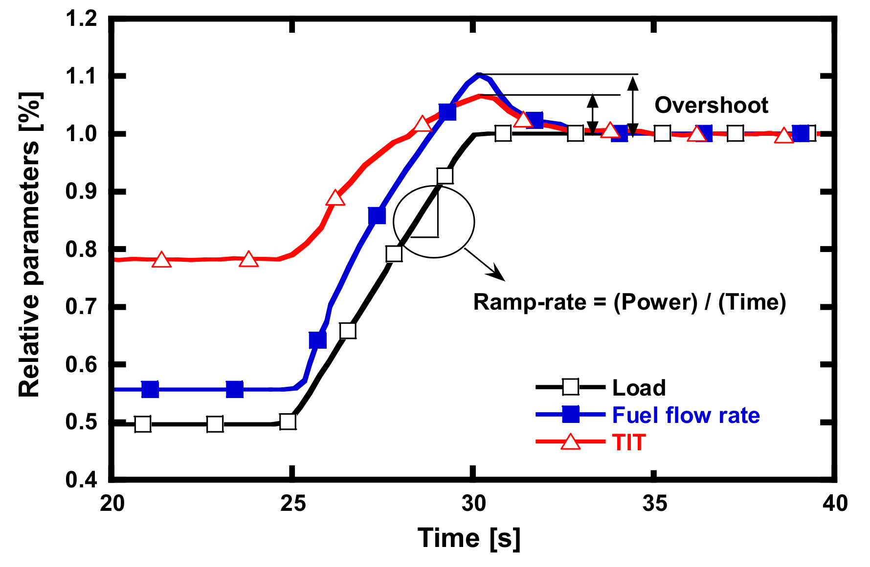
1.2. Increase of GT Ramp-Rate for Operational Flexibility
1.3. Research Objective
2. GT Simulation Model
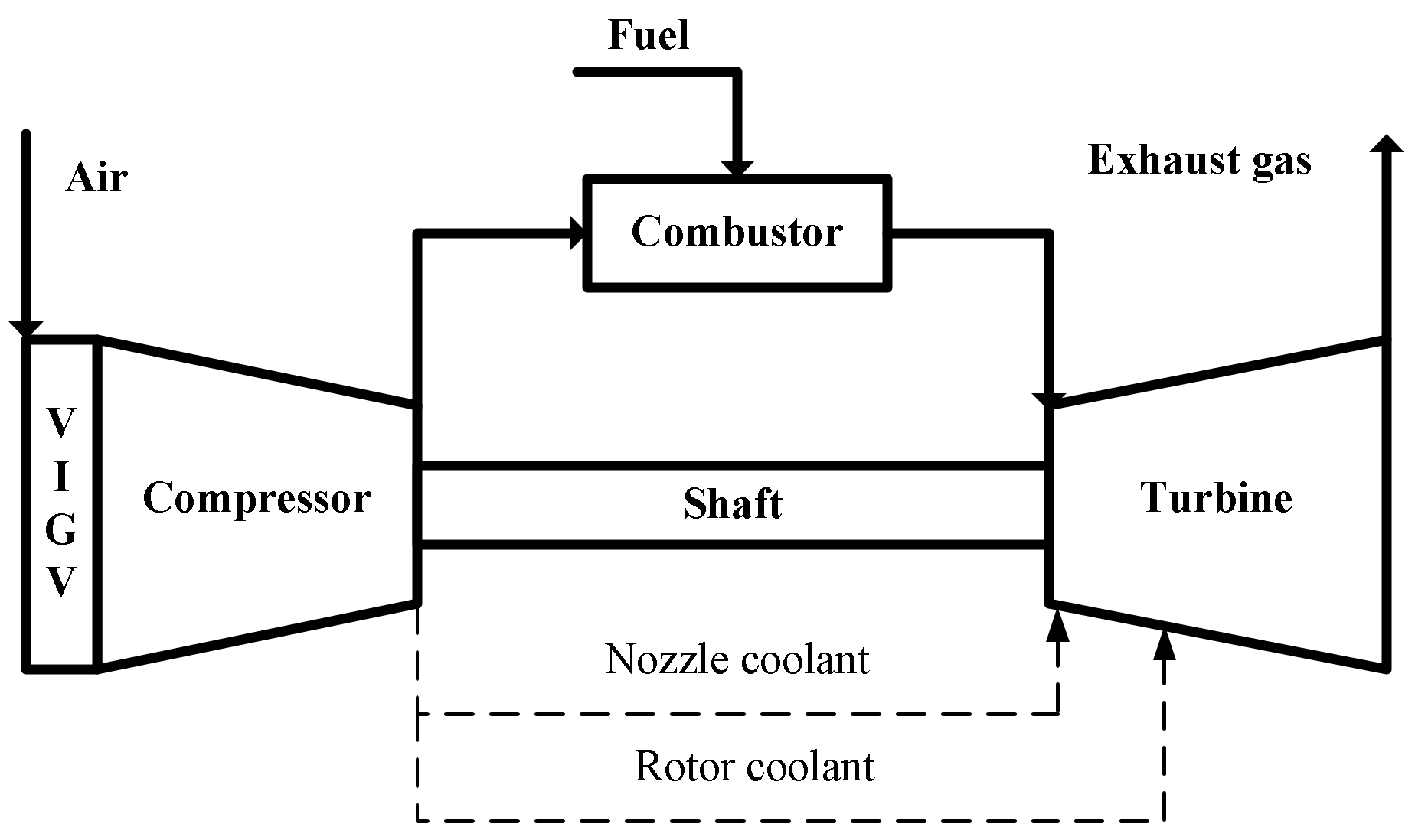
2.1. Design Modeling
2.2. Off-Design Modeling and Validation
2.2.1. Overview
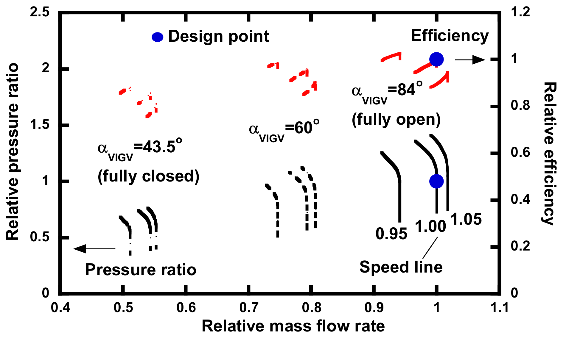
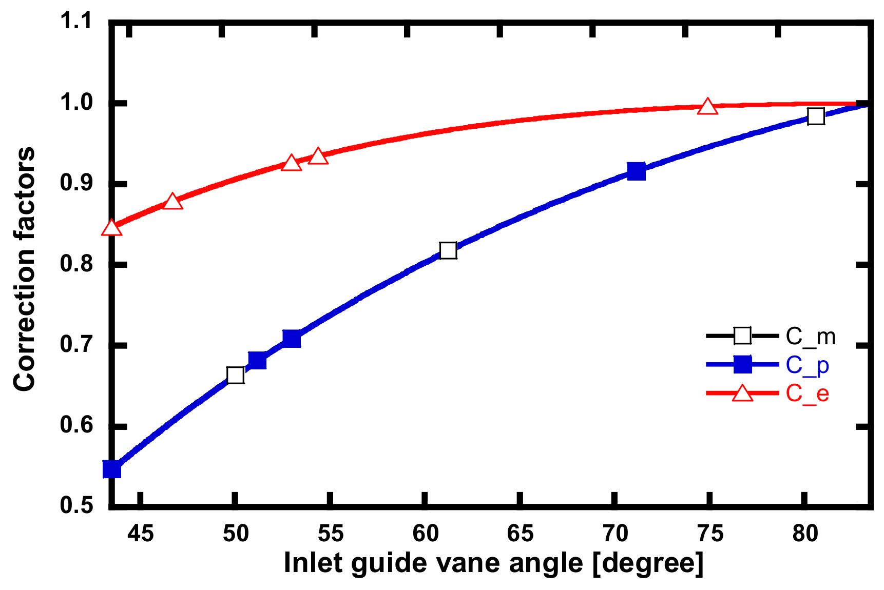
2.2.2. Compressor
2.2.3. Duct
2.2.4. Combustor
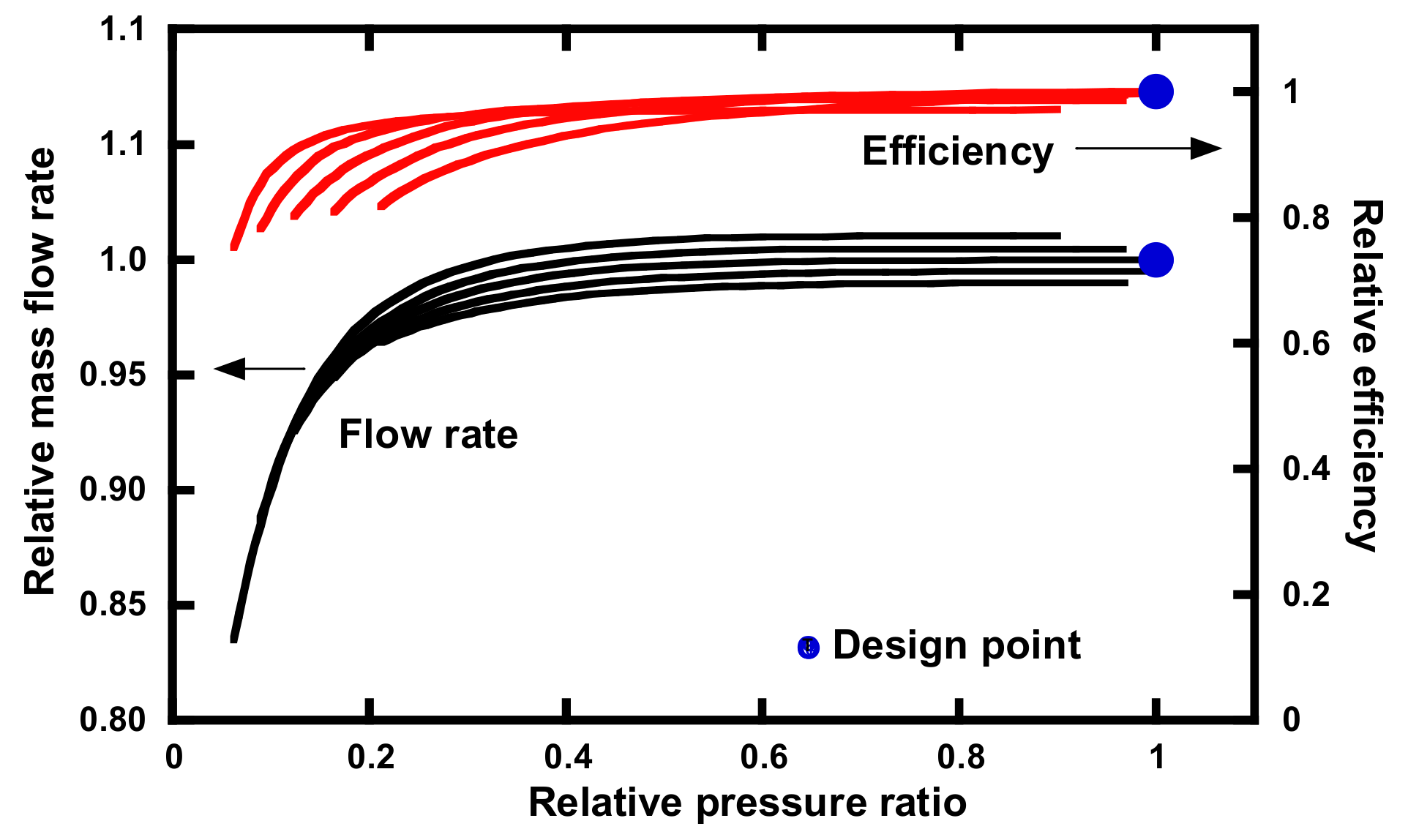
2.2.5. Turbine
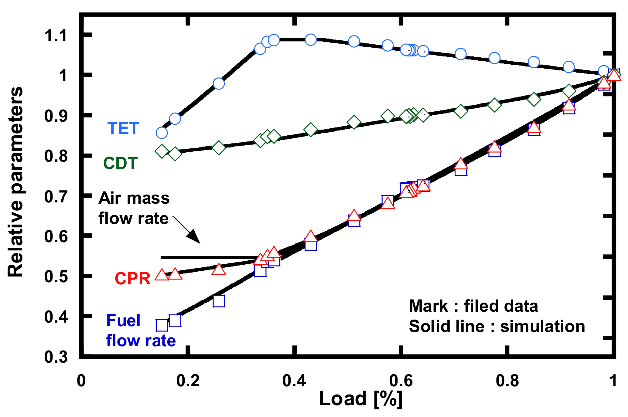
2.2.6. Validation
2.3. Dynamic Modeling
2.3.1. Start-Up Data
2.3.2. Rotating Inertia
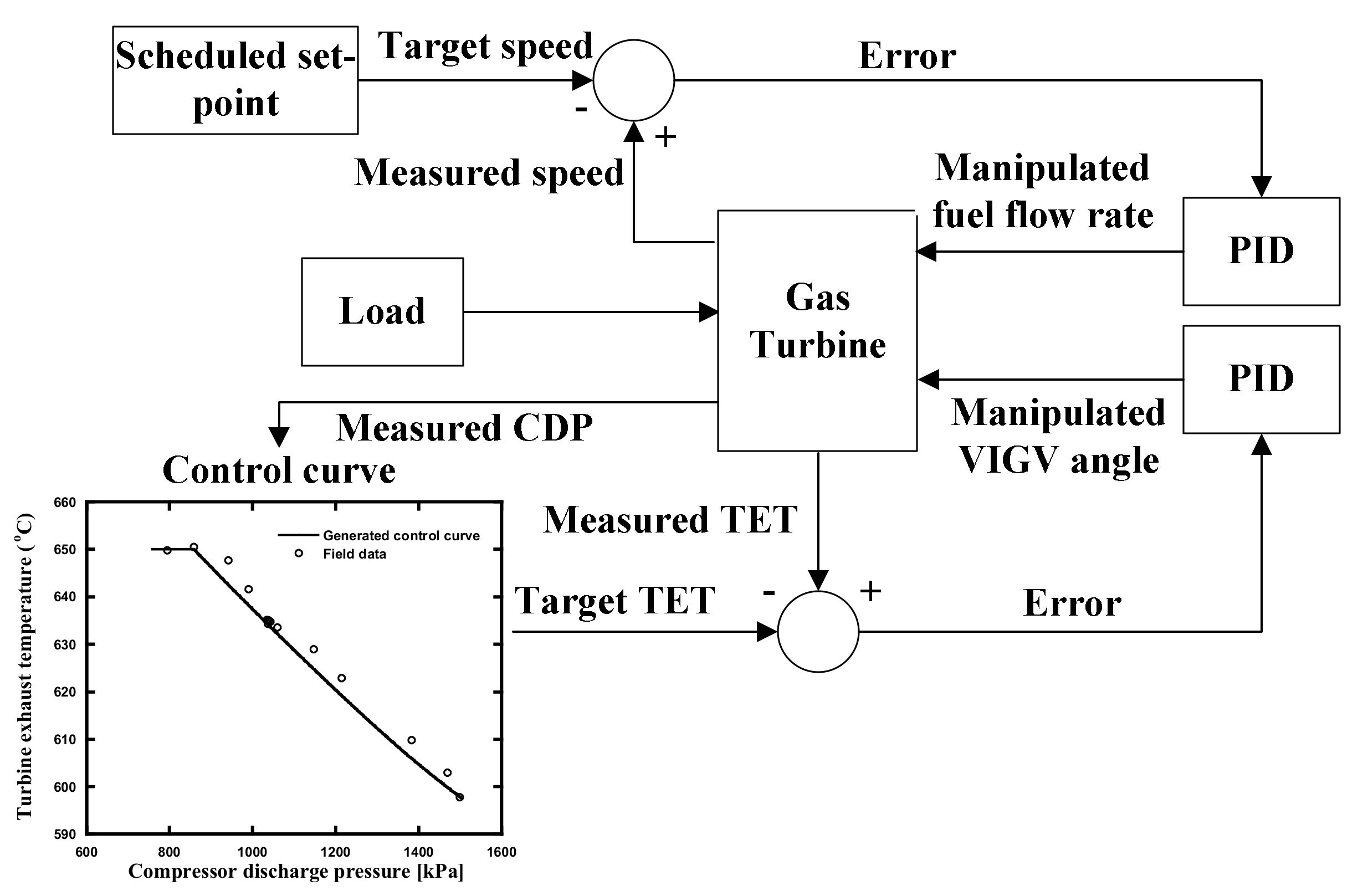
2.3.3. Conventional PID Controller Design (Control Unit)
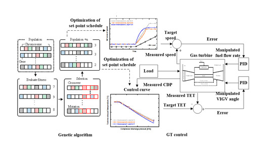
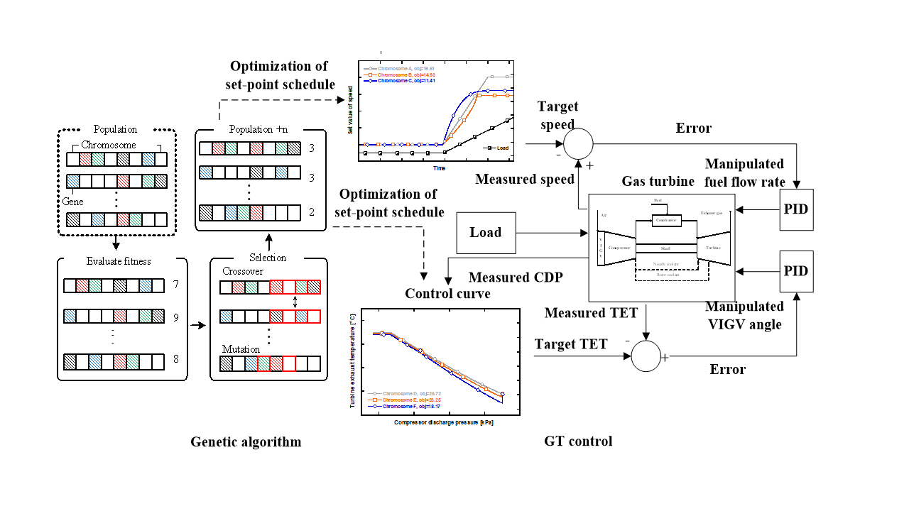
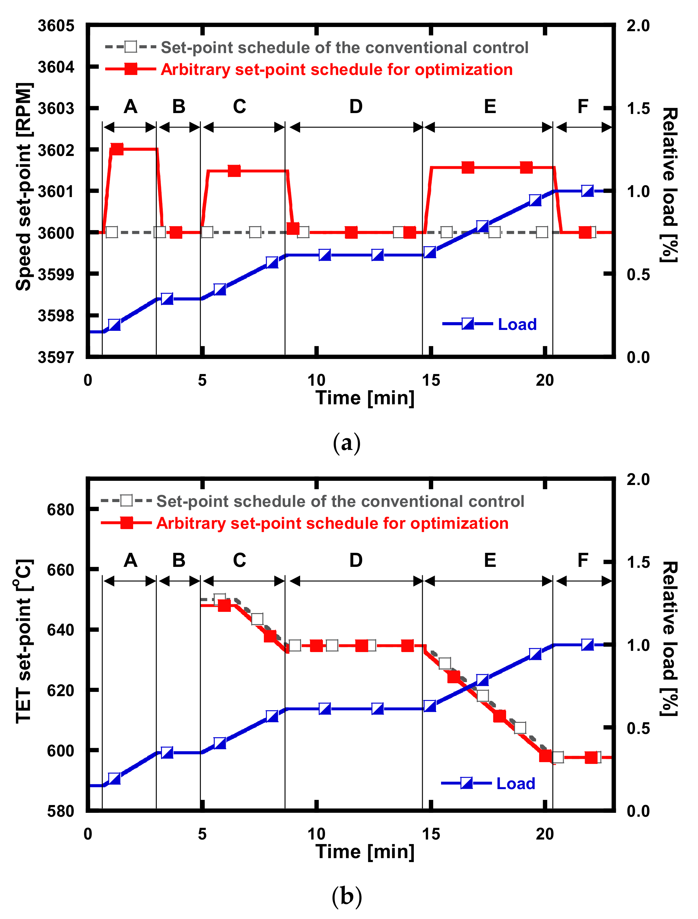
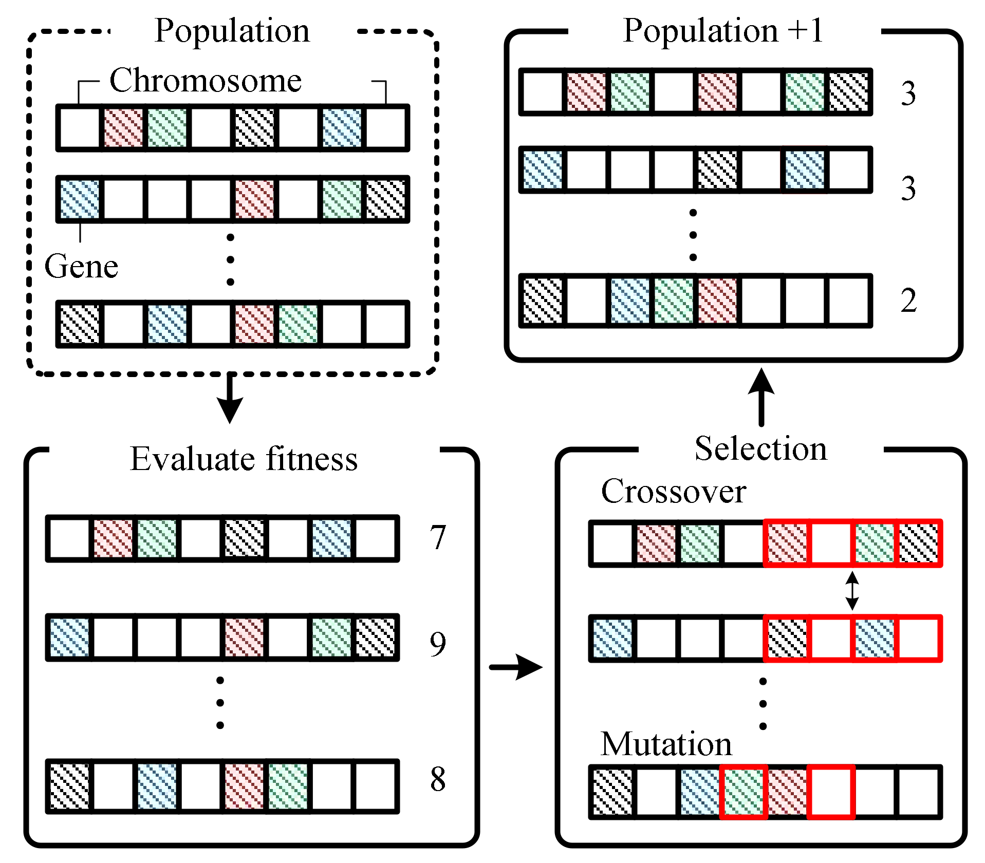
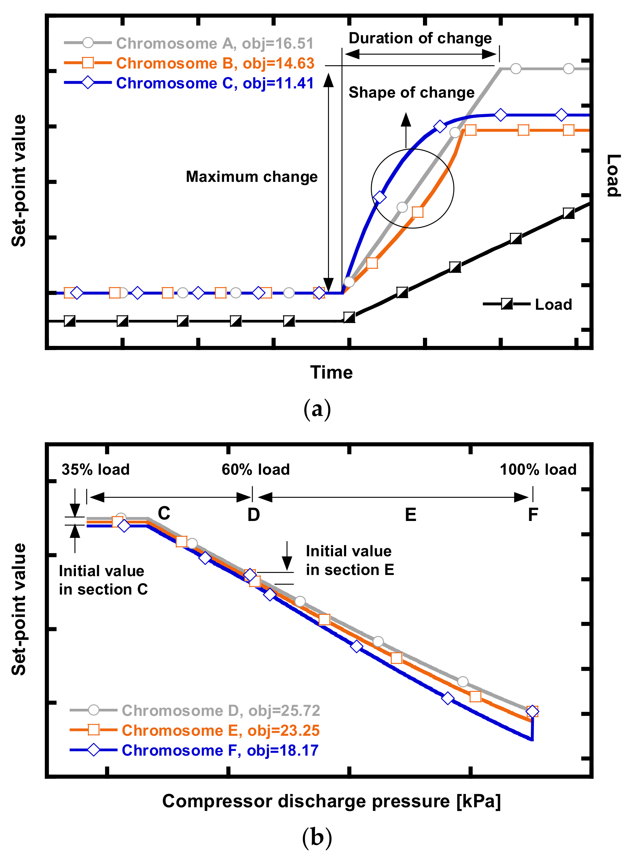
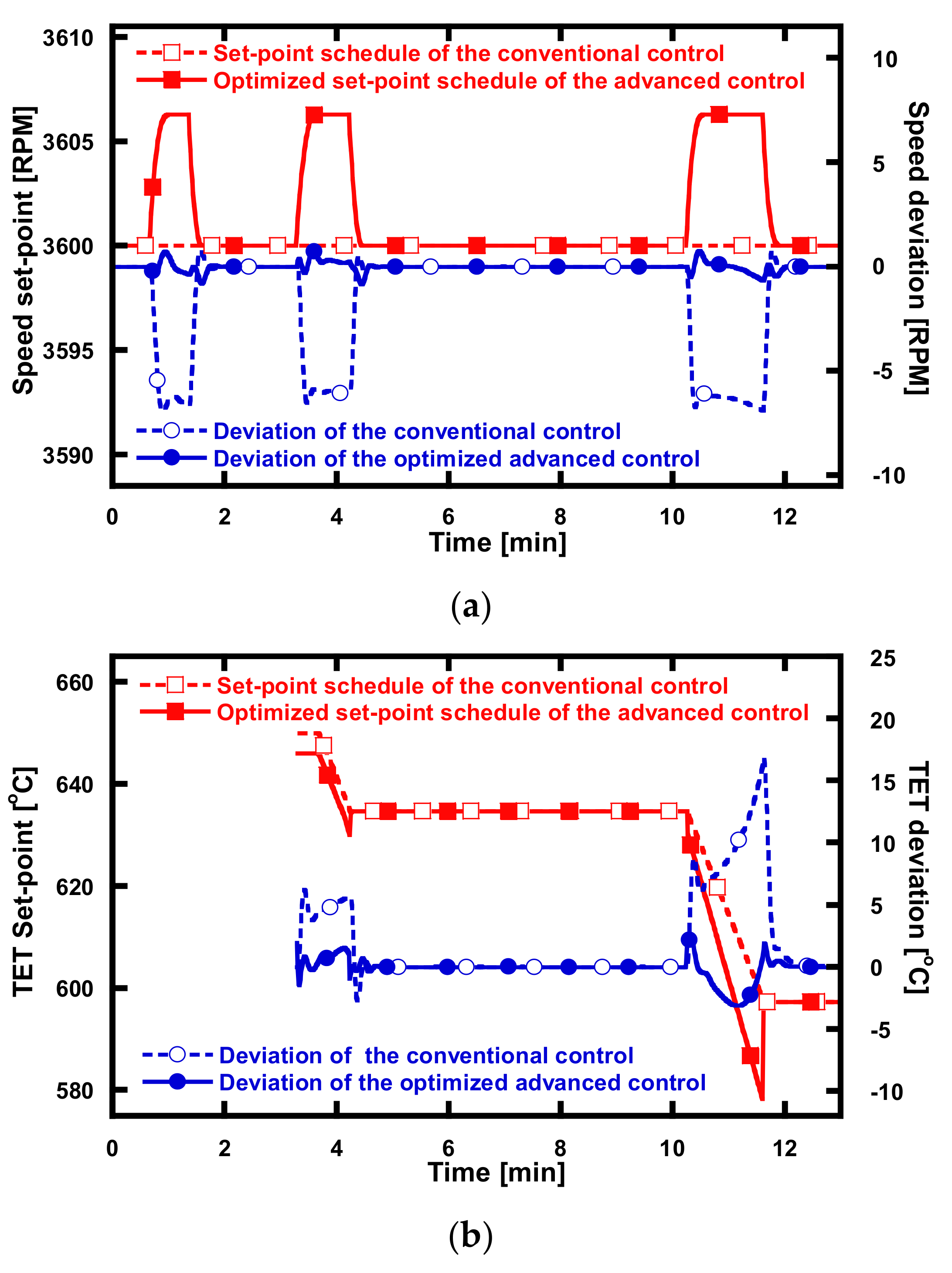
2.3.4. Optimization of the Set-Point Schedule for the Advanced Control
3. Results and Discussion
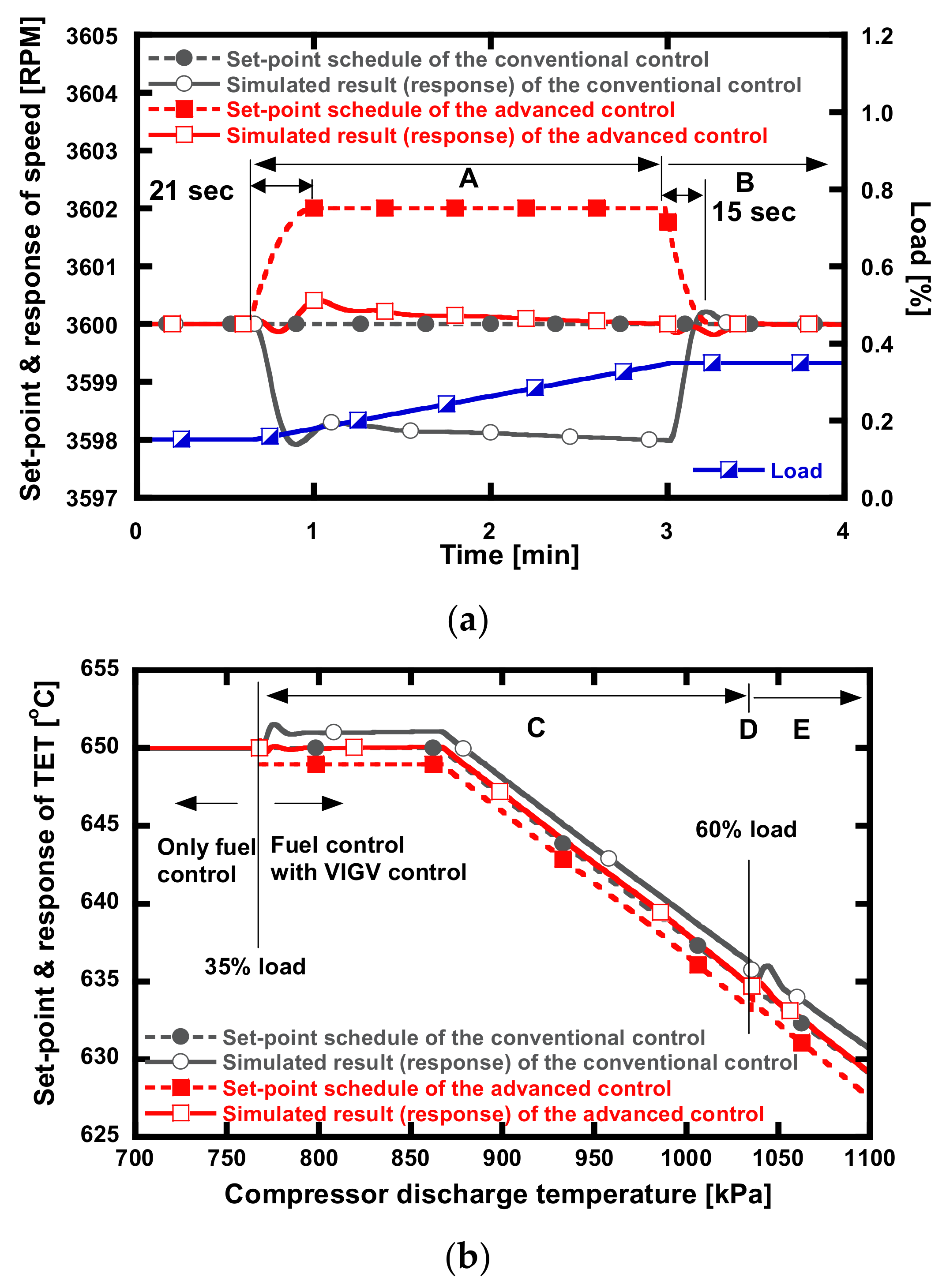
3.1. Impact of the Optimized Control
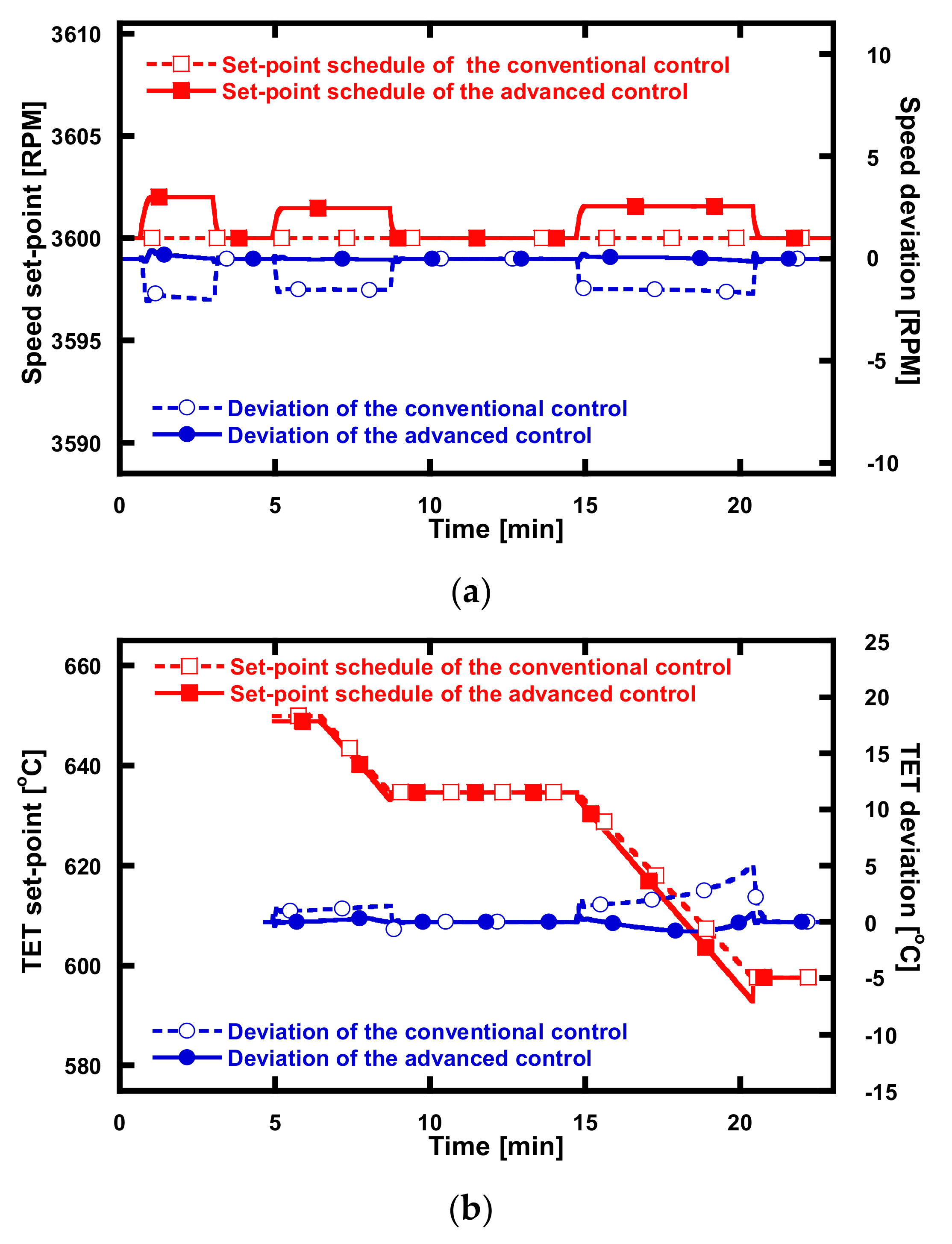
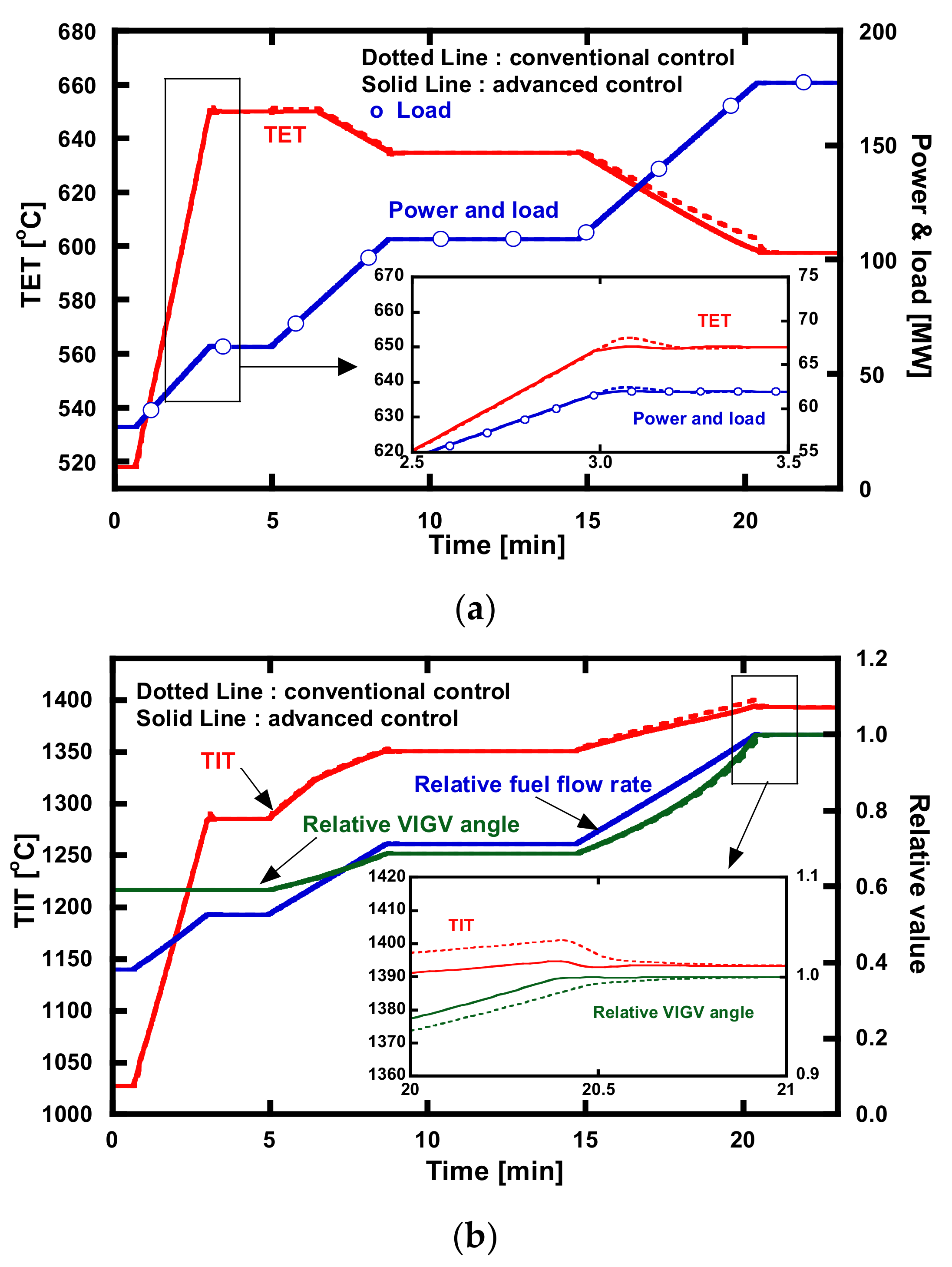
3.2. Effect of Using the Advanced Control for the Reference Ramp-Rates
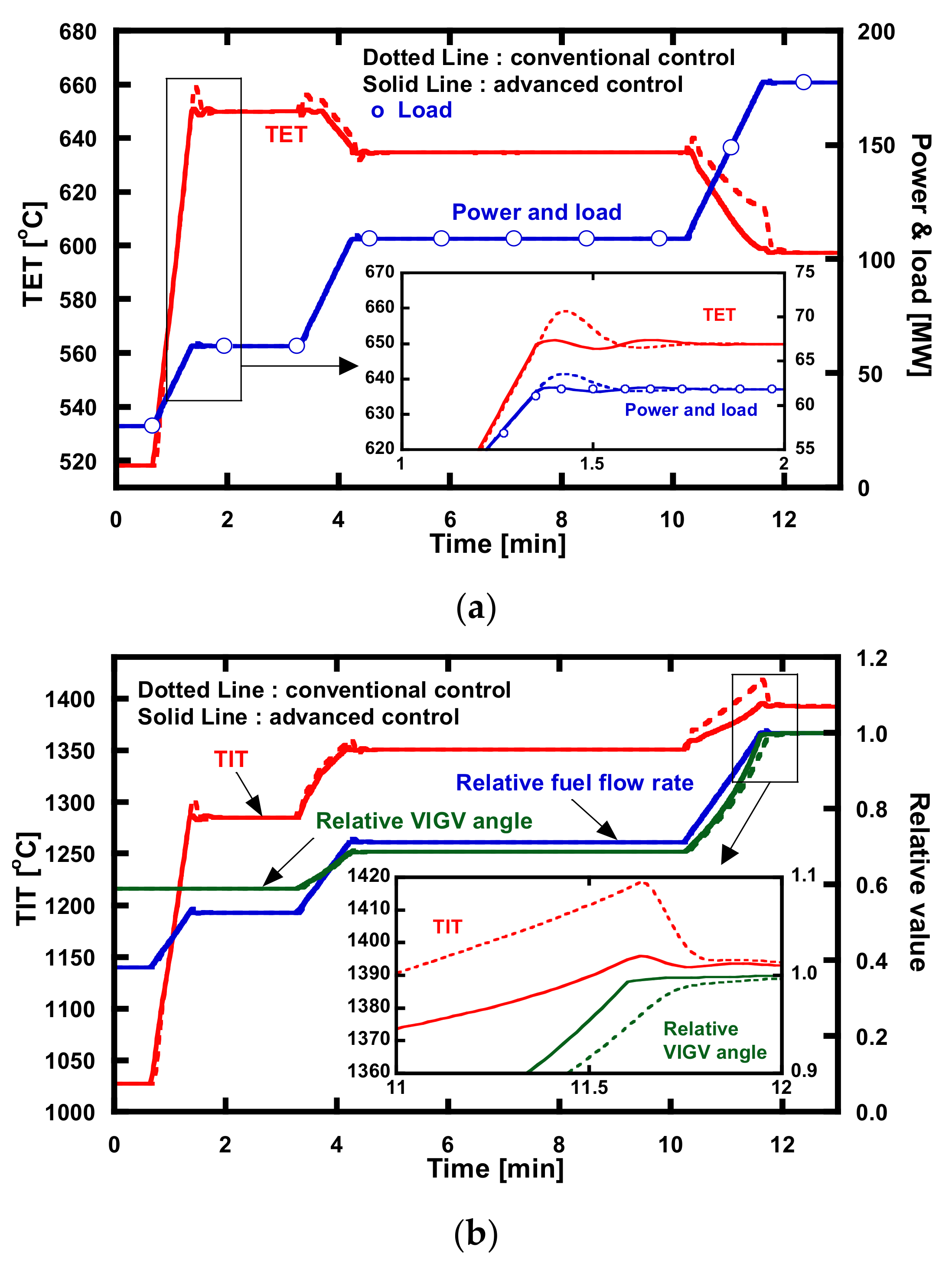
3.3. Effect of Using the Advanced Control for an Increased Ramp-Rate
4. Conclusions
Author Contributions
Funding
Institutional Review Board Statement
Informed Consent Statement
Conflicts of Interest
Nomenclature
| C | Correction factor |
| Energy | |
| e | Error |
| f | Fraction of rotor coolant chargeable to power |
| h | Specific enthalpy (kJ/kg) |
| I | Rotating inertia (kg∙m2) |
| K | Gain |
| Load | Load (kW) |
| M | Semi-dimensionless mass flow rate (kg·K0.5/kN·s) |
| Mass flow rate (kg/s) | |
| MV | Manipulated variable |
| N | Rotation speed (rpm) |
| obj | Objective function |
| P | Pressure (kPa) |
| PR | Pressure ratio |
| PV | Process variable |
| SP | Set-point |
| s | Specific entropy (kJ/kg) |
| T | Temperature (°C) |
| t | Time (sec) |
| Power (kW) | |
| Greek | |
| α | Inlet guide vane angle (°) |
| η | Efficiency (-) |
| Ω | Semi-dimensionless speed (rpm/K0.5) |
| ω | Rotation speed (rad/s) |
| Subscripts | |
| Coolant | Cooling air flow |
| Comb | Combustor |
| Comp | Compressor |
| Conventional | Conventional value |
| Corrected | Corrected value |
| D | Derivative |
| d | Design |
| e | Efficiency |
| field | Field data |
| fuel | Fuel flow |
| GT | Gas turbine |
| I | Integral |
| in | Inlet |
| loss | Losses |
| m | mass flow rate |
| N | Nozzle |
| NC | Nozzle coolant |
| new | New value |
| original | Original value |
| out | Outlet |
| P | Proportional |
| p | Pressure ratio |
| R | Rotor |
| RC | Rotor coolant |
| ref | Reference |
| shaft | Shaft |
| s | Isentropic |
| simulation | Simulation data |
| turb | Turbine |
Abbreviations
| ANN | Artificial neural network |
| CDT | Compressor discharge temperature (°C) |
| CPR | Compressor pressure ratio |
| GT | Gas turbine |
| LHV | Lower heating value (kJ/kg) |
| PID | Proportional-integral-derivative |
| P2G | Power to gas |
| P2L | Power to liquid |
| RMSD | Root mean square deviation |
| TET | Turbine exhaust temperature (°C) |
| TIT | Turbine inlet temperature (°C) |
| VIGV | Variable inlet guide vane |
References
- International Energy Agency. World Energy Outlook; International Energy Agency: Paris, France, 2020; pp. 1–464. [Google Scholar]
- Wang, Y.; Silva, V.; Lopez-Botet-zulueta, M. Impact of high penetration of variable renewable generation on frequency dynamics in the continental Europe interconnected system. IET Renew. Power Gener. 2016, 10, 10–16. [Google Scholar] [CrossRef]
- Sinsel, S.R.; Riemke, R.L.; Hoffmann, V.H. Challenges and solution technologies for the integration of variable renewable energy sources—A review. Renew. Energy 2020, 145, 2271–2285. [Google Scholar] [CrossRef]
- Isaiah, T.G.; Dabbashi, S.; Bosak, D.; Sampath, S.; Di Lorenzo, G.; Pilidis, P. Life Analysis of Industrial Gas Turbines Used as a Back-Up to Renewable Energy Sources. Procedia CIRP 2015, 38, 239–244. [Google Scholar] [CrossRef]
- Jenkins, J.D.; Zhou, Z.; Ponciroli, R.; Vilim, R.B.; Ganda, F.; de Sisternes, F.; Botterud, A. The benefits of nuclear flexibility in power system operations with renewable energy. Appl. Energy 2018, 222, 872–884. [Google Scholar] [CrossRef]
- Wang, B.; Zhang, C.; Dong, Z.Y.; Li, X. Improving Hosting Capacity of Unbalanced Distribution Networks via Robust Allocation of Battery Energy Storage Systems. IEEE Trans. Power Syst. 2021, 36, 2174–2185. [Google Scholar] [CrossRef]
- Bizon, N.; Hoarcă, I.C. Hydrogen saving through optimized control of both fueling flows of the Fuel Cell Hybrid Power System under a variable load demand and an unknown renewable power profile. Energy Convers. Manag. 2019, 184, 1–14. [Google Scholar] [CrossRef]
- Ulbig, A.; Borsche, T.S.; Andersson, G. Impact of low rotational inertia on power system stability and operation. IFAC Proc. 2014, 19, 7290–7297. [Google Scholar] [CrossRef]
- Johnson, S.C.; Papageorgiou, D.J.; Mallapragada, D.S.; Deetjen, T.A.; Rhodes, J.D.; Webber, M.E. Evaluating rotational inertia as a component of grid reliability with high penetrations of variable renewable energy. Energy 2019, 180, 258–271. [Google Scholar] [CrossRef]
- Ulbig, A.; Rinke, T.; Chatzivasileiadis, S.; Andersson, G. Predictive control for real-time frequency regulation and rotational inertia provision in power systems. In Proceedings of the IEEE Conference on Decision and Control, Firenze, Italy, 10–13 December 2013; pp. 2946–2953. [Google Scholar] [CrossRef]
- Boubenia, A.; Hafaifa, A.; Kouzou, A.; Mohammedi, K.; Becherif, M. Carbone dioxide capture and utilization in gas turbine plants via the integration of power to gas. Petroleum 2017, 3, 127–137. [Google Scholar] [CrossRef]
- Albrecht, F.G.; Konig, D.H.; Dietrich, R.U. The potential of using power-to-liquid plants for power storage purposes. In Proceedings of the International Conference on the European Energy Market, EEM, Porto, Portugal, 6–9 June 2016; pp. 1–5. [Google Scholar] [CrossRef][Green Version]
- Ahn, J.H.; Jeong, J.H.; Kim, T.S. Performance Enhancement of a Molten Carbonate Fuel Cell/Micro Gas Turbine Hybrid System with Carbon Capture by Off-Gas Recirculation. J. Eng. Gas Turbines Power 2019, 141, 1–10. [Google Scholar] [CrossRef]
- Bexten, T.; Wirsum, M.; Rosche, B.; Schelenz, R.; Jacobs, G. Model-Based Analysis of a Combined Heat and Power System Featuring a Hydrogen-Fired Gas Turbine with On-Site Hydrogen Production and Storage. In Proceedings of the ASME Turbo Expo, virtual, 21–25 September 2020. [Google Scholar]
- California Independent System Operator. What the Duck Curve Tells Us about Managing a Green Grid; California Independent System Operator: Folsom, CA, USA, 2016. [Google Scholar]
- Scottmadden Inc. Revisiting the California Duck Curve; ScottMadden: Atlanta, GA, USA, 2016. [Google Scholar]
- GE GAS POWER. OpFlex* Advanced Control Solutions. 2021. Available online: https://www.ge.com/content/dam/gepower-new/global/en_US/downloads/gas-new-site/products/digital-and-controls/opflex/opflex-brochure.pdf (accessed on 25 November 2021).
- Power Engineering International. Siemens Blends Past and Present for Next Generation Gas-Fired Power Efficiency. 12 January 2018. Available online: https://www.powerengineeringint.com/coal-fired/siemens-blends-past-and-present-for-next-generation-gas-fired-power-efficiency/ (accessed on 20 November 2021).
- Rowen, W.I. Simplified mathematical representations of single shaft gas turbines in mechanical drive service. In Proceedings of the ASME International Gas Turbine and Aeroengine Congress and Exposition, Cologne, Germany, 1–4 June 1992. [Google Scholar]
- Kim, T.S. Comparative analysis on the part load performance of combined cycle plants considering design performance and power control strategy. Energy 2004, 29, 71–85. [Google Scholar] [CrossRef]
- Camporeale, S.M.; Fortunato, B.; Mastrovito, M. A modular code for real time dynamic simulation of gas turbines in simulink. J. Eng. Gas Turbines Power 2006, 128, 506–517. [Google Scholar] [CrossRef]
- Baggini, A. Handbook of Power Quality; Wiley: New York, NY, USA, 2008; ISBN 9780470754238. [Google Scholar]
- Kavalerov, B.V.; Bakhirev, I.V.; Kilin, G.A. An investigation of adaptive control of the rotation speed of gas turbine power plants. Russ. Electr. Eng. 2016, 87, 607–611. [Google Scholar] [CrossRef]
- Townsend, R.; Winstone, M.; Henderson, M.; Nicholls, J.R.; Partridge, A.; Nath, B.; Wood, M.; Viswanathan, R. Life Assessment of Hot Section Gas Turbine Components; Cambridge University Press: Cambridge, UK, 2000; pp. 37–38. Available online: https://www.scopus.com/record/display.uri?eid=2-s2.0-85064348601&origin=inward (accessed on 20 November 2021).
- Mohamed, W.; Eshati, S.; Pilidis, P.; Ogaji, S.; Laskaridis, P.; Nasir, A. A method to evaluate the impact of power demand on HPT blade creep life. In Proceedings of the ASME Turbo Expo, Vancouver, QC, Canada, 6–10 June 2011; Volume 4, pp. 1–45092. [Google Scholar]
- Abdul Ghafir, M.F. Performance Based Creep Life Estimation for Gas Turbine Application. Ph.D. Thesis, Cranfield University, Bedford, UK, 2011. Available online: https://ethos.bl.uk/OrderDetails.do?uin=uk.bl.ethos.566015 (accessed on 20 November 2021).
- Benato, A.; Bracco, S.; Stoppato, A.; Mirandola, A. LTE: A procedure to predict power plants dynamic behaviour and components lifetime reduction during transient operation. Appl. Energy 2016, 162, 880–891. [Google Scholar] [CrossRef]
- Wood, M.I. Gas turbine hot section components: The challenge of ‘residual life’ assessment. Proc. Inst. Mech. Eng. Part A J. Power Energy 2000, 214, 193–201. [Google Scholar] [CrossRef]
- Rossi, I.; Source, A.; Traverso, A. Gas turbine combined cycle start-up and stress evaluation a simplified dynamic approach. Appl. Energy 2017, 190, 880–890. [Google Scholar] [CrossRef]
- Poursaeidi, E.; Bazvandi, H. Effects of emergency and fired shut down on transient thermal fatigue life of a gas turbine casing. Appl. Therm. Eng. 2016, 100, 453–461. [Google Scholar] [CrossRef]
- Kim, M.J.; Kim, T.S. Feasibility study on the influence of steam injection in the compressed air energy storage system. Energy 2017, 141, 239–249. [Google Scholar] [CrossRef]
- Moon, S.W.; Kim, T.S. Advanced Gas Turbine Control Logic Using Black Box Models for Enhancing Operational Flexibility and Stability. Energies 2020, 13, 5703. [Google Scholar] [CrossRef]
- Eldrid, R.; Kaufman, L.; Marks, P. The 7FB: The Next Evolution of the F Gas Turbine; GE Power Systems: Schenectady, NY, USA, 2001. [Google Scholar]
- Gay, R.R.; Palmer, C.A.; Erbes, M.R. Power Plant Performance Monitoring; Techniz Books International: New Delhi, India, 2006; pp. 110–116. ISBN 0-9755876-0-9. [Google Scholar]
- Moon, S.W.; Kwon, H.M.; Kim, T.S.; Kang, D.W.; Sohn, J.L. A novel coolant cooling method for enhancing the performance of the gas turbine combined cycle. Energy 2018, 160, 625–634. [Google Scholar] [CrossRef]
- Lee, J.H.; Kim, T.S. Novel performance diagnostic logic for industrial gas turbines in consideration of over-firing. J. Mech. Sci. Technol. 2018, 32, 5947–5959. [Google Scholar] [CrossRef]
- Kim, J.H.; Kim, T.S.; Moon, S.J. Development of a program for transient behavior simulation of heavy-duty gas turbines. J. Mech. Sci. Technol. 2016, 30, 5817–5828. [Google Scholar] [CrossRef]
- MathWorks Inc. MATLAB R2021a; MathWorks Inc.: Natick, MA, USA, 2021; Available online: https://mathworks.com/products/matlab.html (accessed on 20 November 2021).
- Kim, M.J.; Kim, J.H.; Kim, T.S. Program development and simulation of dynamic operation of micro gas turbines. Appl. Therm. Eng. 2016, 108, 122–130. [Google Scholar] [CrossRef]
- McBride, B.J.; Zehe, M.J.; Gordon, S. NASA Glenn Coefficient for Calculating Thermodynamic Properties of Individual Species; Glenn Research Center: Cleveland, OH, USA, 2002. [Google Scholar]
- Petkovic, D.; Banjac, M.; Milic, S.; Petrovic, M.V.; Wiedermann, A. Modelling the transient behaviour of gas turbines. In Proceedings of the ASME Turbo Expo, Phoenix, AZ, USA, 17–21 June 2019; pp. 1–91008. [Google Scholar]
- Agrawal, R.K.; Yunis, M. A generalized mathematical model to estimate gas turbine starting characteristics. In Proceedings of the ASME Turbo Expo, Houston, Texas, USA, 9–12 March 1981; pp. 194–202. [Google Scholar]
- Saravanamuttoo, H.I.; MacIsaac, B.D. The use of a hybrid computer in the optimization of gas turbine control parameters. Asme J. Eng. Power 1973, 95, 257–264. [Google Scholar] [CrossRef]
- GasTurb GmbH. GasTurb12; GasTurb GmbH: Aachen, Germany, 2012. [Google Scholar]
- GE Energy. GateCycle ver. 6.1.2.; General Electric: Boston, MA, USA, 2013. [Google Scholar]
- Tarabrin, A.P.; Schurovsky, V.A.; Bodrov, A.I.; Stalder, J.P. Influence of axial compressor fouling on gas turbine unit performance based on different schemes and with different initial parameters. Am. Soc. Mech. Eng. 1998, 78651, 317–325. [Google Scholar] [CrossRef]
- Saravanamuttoo, H.I.; Rogers, G.F.C.; Cohen, H. Gas Turbine Theory; Pearson Education: London, UK, 2001; ISBN 978-1292093093. [Google Scholar]
- Turns, S.R. An Introduction to Combustion: Concepts and Applications, 2nd ed.; McGraw-Hill: New York, NY, USA, 2000; ISBN 10:007235044X. [Google Scholar]
- Palmer, C.A.; Erbes, M.R. Simulation Methods Used to Analyze the Performance of the GE PG6541B Gas Turbine Utilizing Low Heating Value Fuels. In Proceedings of the ASME Cogen Turbo Power, Portland, OR, USA, 25–27 October 1994; pp. 1–8. [Google Scholar]
- Zucca, A.; Khayrulin, S.; Vyazemskaya, N.; Shershnyov, B.; Myers, G. Development of a liquid fuel system for GE MS5002E gas turbine: Rig test validation of the combustor performance. In Proceedings of the ASME Turbo Expo, Düsseldorf, Germany, 16–20 June 2014; pp. 1–8. [Google Scholar] [CrossRef]
- Lahyani, A.; Boughaleb, Y.; Qjani, M. Dynamic Model of a Two Shaft Heavy-Duty Gas Turbine with Variable Geometry. In Proceedings of the International Gas Turbine and Aeroengine Congress and Exposition, Houston, TX, USA, 5 June 1995. [Google Scholar]
- Kim, J.H.; Song, T.W.; Ro, S.T. Model development and simulation of transient behavior of heavy duty gas turbines. J. Eng. Gas Turbines Power 2001, 123, 589–594. [Google Scholar] [CrossRef]
- Panov, V. Gasturbolib—Simulink library for gas turbine engine modelling. In Proceedings of the ASME Turbo Expo, Orlando, FL, USA, 8–12 June 2009; Volume 1, pp. 555–59389. [Google Scholar]
- Bank Tavakoli, M.R.; Vahidi, B.; Gawlik, W. An educational guide to extract the parameters of heavy duty gas turbines model in dynamic studies based on operational data. IEEE Trans. Power Syst. 2009, 24, 1366–1374. [Google Scholar] [CrossRef]
- Rowen, W.I. Operating characteristics of heavy-duty gas turbines in utility service. In Proceedings of the ASME Turbo Expo, Birmingham, UK, 2–5 June 1988; pp. 5–150. [Google Scholar]
- MathWorks, Inc. Global Optimization Toolbox: User’s Guide (R2021b); MathWorks Inc.: Natick, MA, USA, 2021; Available online: https://www.mathworks.com/help/pdf_doc/gads/gads.pdf (accessed on 20 November 2021).


| Parameters | Field Data | In House Code |
|---|---|---|
| Ambient temperature [°C] | 15 | 15 |
| Ambient pressure [kPa] | 101.325 | 101.325 |
| Ambient relative humidity [%] | 60 | 60 |
| Air mass flow rate [kg/s] | N/A | 421.371 [37] |
| Compressor pressure ratio [-] | 15.2 | 15.2 |
| Compressor polytropic efficiency [%] | 91.84 | 91.84 |
| Fuel flow rate [kg/s] | 9.1437 | 9.1437 |
| Turbine inlet temperature [°C] | N/A | 1397 [37] |
| Turbine rotor blade inlet temperature [°C] | N/A | 1327 [37] |
| Turbine exhaust gas temperature [°C] | 608.1 | 608.1 |
| Turbine polytropic efficiency [%] | N/A | 88.57 |
| Total cooling air flow rate [kg/s] | N/A | 81.84 |
| Shaft speed [rpm] | 3600 | 3600 |
| Mechanical efficiency [%] | N/A | 99 [37] |
| Generator efficiency [%] | N/A | 98.5 [37] |
| Net power [MW] | 166.4 | 166.4 |
| Gas turbine Efficiency (LHV) [%] | 36.91 | 36.91 |
| Parameters (Maximum Value) | Reference Ramp-Rates (15 MW/min and 12 MW/min) | Increased Ramp-Rate (50 MW/min) | ||
|---|---|---|---|---|
| Conventional Control | Advanced Control | Conventional Control | Advanced Control | |
| [%] | 0.30 | 0.13 | 1.24 | 0.42 |
| Speed deviation [%] | 0.06 | 0.01 | 0.19 | 0.02 |
| TET [°C] | 652.8 | 650.5 | 659.2 | 651.9 |
| TIT [°C] | 1401.1 | 1394.8 | 1418.6 | 1395.9 |
| Rate of TIT change [°C/s] | 0.7 | 0.4 | 2.3 | 0.6 |
Publisher’s Note: MDPI stays neutral with regard to jurisdictional claims in published maps and institutional affiliations. |
© 2021 by the authors. Licensee MDPI, Basel, Switzerland. This article is an open access article distributed under the terms and conditions of the Creative Commons Attribution (CC BY) license (https://creativecommons.org/licenses/by/4.0/).
Share and Cite
Park, Y.-K.; Moon, S.-W.; Kim, T.-S. Advanced Control to Improve the Ramp-Rate of a Gas Turbine: Optimization of Control Schedule. Energies 2021, 14, 8024. https://doi.org/10.3390/en14238024
Park Y-K, Moon S-W, Kim T-S. Advanced Control to Improve the Ramp-Rate of a Gas Turbine: Optimization of Control Schedule. Energies. 2021; 14(23):8024. https://doi.org/10.3390/en14238024
Chicago/Turabian StylePark, Young-Kwang, Seong-Won Moon, and Tong-Seop Kim. 2021. "Advanced Control to Improve the Ramp-Rate of a Gas Turbine: Optimization of Control Schedule" Energies 14, no. 23: 8024. https://doi.org/10.3390/en14238024
APA StylePark, Y.-K., Moon, S.-W., & Kim, T.-S. (2021). Advanced Control to Improve the Ramp-Rate of a Gas Turbine: Optimization of Control Schedule. Energies, 14(23), 8024. https://doi.org/10.3390/en14238024