Reservoir Simulation of CO₂ Storage Using Compositional Flow Model for Geological Formations in Frio Field and Precaspian Basin

Abstract

CO${}_2$ storage is a greenhouse gas mitigation instrument for many countries. In this paper, we investigate the possibility of CO${}_2$ storage in the region of the Precaspian basin using the compositional flow model that was verified by the data of the Frio pilot project, USA. We use local grid refinement in the commercial reservoir simulator. In the reservoir simulation for data of the Frio Pilot project, we have achieved a good history matching of well pressure. Different scenarios were tested, and post-injection migration was shown for both case studies. The long-term reservoir simulation shows the potential amount of trapped CO${}_2$ by residual and dissolved trapping mechanisms in the Precaspian basin. The performed uncertainty study covered the uncertainty of the model’s parameters resulting in P10, P50 and P90 cases in terms of the amount of trapped CO${}_2$.

1. Introduction

In the last few years, there has been a growing interest in studying many mechanisms to achieve reductions in CO${}_2$ concentration in the atmosphere. The growing infrastructure of countries requires increased consumption of fossil fuels that can result in the greenhouse effect. Efforts of many countries in controlling greenhouse gas emissions were documented in the Paris Agreement. One of the methods to mitigate CO${}_2$ emissions is to inject CO${}_2$ into the geological storage including depleted oil and gas reservoirs or aquifer formations. The injection of CO${}_2$ should be at sufficient depth to allow CO${}_2$ to be in a supercritical state (in general, the depth should approximately be larger than 800 m so that the pressure is above 7.4 MPa and the temperature is above 31 degrees Celsius) in which the storage capacity is maximized. CO${}_2$ has a liquid-like density and gas-like viscosity in the supercritical state and occupies approximately one hundredth of the volume it does as a gas at standard conditions. The recognition of the viable role of carbon sequestration is increasing, and the implementation of such technologies can be found in many projects around world from USA, UK, China, Norway, etc. In [1], the method for evaluating CO${}_2$ storage capacity was proposed in the global context in order to achieve “two degree scenario” objective.

The assessment of the storage capacity is sophisticated since there are many trapping strategies. We highlight four main trapping mechanisms of carbon dioxide in the aquifer such as hydrodynamic trapping when CO${}_2$ migrates upwards and remains just below the cap rock (a structural or stratigraphic trap must exist); immobile phase as residual gas saturation during the imbibition process; dissolution in water; and mineral trapping. The first three trapping mechanisms are the most important instruments as the mineral trapping effects can be observed only after a long period of time (many years, maybe even thousand of years). The most desirable mechanisms for trapping are immobile phase and dissolution in water, because hydrodynamic trapping is risky as the cap rock can partially seal; hence, CO${}_2$ can migrate through it, and its storage efficiency can be reduced.

To address modeling CO${}_2$ storage in the subsurface, many researchers have proposed various numerical models with different realistic data [1,2,3,4]. There are many case studies of such mechanisms around the world such as Johansen formation [5], Utsira formation [6], Cranfield pilot project [7,8], Frio pilot project [9] and others. Large-scale modeling helps to evaluate the behavior of the injected CO${}_2$ in various scenarios, and the models were verified by using additional sources of field projects including the pressure measurements, seismic surveys, etc.

Kazakhstan’s plan on fulfilling the Paris Agreement (2016) may require additional actions in order to be able to achieve the goals of achieving a 25% emission reduction strategy by 2030. According to [10], the current mitigation activities in Kazakhstan may not be enough to reach a reduction of 15% (unconditional target) based on the business as usual(BaU) model. CO${}_2$ sequestration can be a solution for the country in the reduction in CO${}_2$ emissions. Potential locations in Kazakhstan for CO${}_2$ storage were discussed in [11,12], and the locations were estimated to possess around 1003 Mt CO${}_2$ storage capacity of the gas reservoirs of Kazakhstan in [13]. However, most of previous studies do not take into account numerical reservoir simulations of CO${}_2$ storage in Kazakhstan.

In this study, we investigate the reservoir simulation of CO${}_2$ storage in 3D using the compositional flow model for the Frio CO${}_2$ project in the USA and the Precaspian Basin in Kazakhstan. We study the effect of parameters that can be essential in modeling CO${}_2$ storage evaluation in a potential subsurface of Kazakhstan. Model verification was performed by history matching of the well pressure profile based on the data of the Frio field experiment. We utilize the commercial simulator Eclipse 300. To the authors’ knowledge, 3D numerical simulation of CO${}_2$ sequestration in the Prescaspian formation has been scarcely investigated from the point of view of evaluating capacity. We propose the potential location of the CO${}_2$ storage and demonstrate the possible amount of trapped CO${}_2$ and present also plume migration in the post-injection period. The possible amount of trapped CO${}_2$ was presented in terms of P10, P50 and P90 cases resulting from the uncertainty study that covered the most uncertain parameters of the reservoir simulation model. This study uses machine learning algorithms to conduct sensitivity analysis incorporated with the reservoir simulator.

The remainder of the paper is organized as follows. Section 2 describes settings in the compositional flow reservoir simulation. We use the data from the Frio CO${}_2$ project as a case study. Reservoir simulation results for regions from the Frio and Precaspian formation are presented in Section 3. The compositional flow model was verified and applied to Frio CO${}_2$ Project, and then it was applied to the Precaspian formation, Kazakhstan. Section 4 summarizes the results of this study and draws conclusions.

2. Model Description

In this section, we provide an overview of the upper part of the Frio formation in USA and describe the compositional flow model setup and input parameters used for the simulation.

2.1. Overview of the Frio CO${}_2$ Model

The injection pilot project in Frio brine formation is used as a case study for reservoir simulation of CO${}_2$ sequestration. The Frio brine field is a sandstone formation with high porosity and permeability and is located in Houston, TX, USA. In this pilot project, 1600 tons of CO${}_2$ was injected during 10 days into the formation 1500 m below the surface (see for more details [14]). The target for injection was the upper Frio Formation (“C” sandstone), which is a 23-meters thick brine-bearing interval above an oil production zone. The upper part of the “C” formation has a porosity of 30 to 35% and permeability of 2000 to 2500 md. There is also some finer grained sandstone with porosity of 24 to 28% and permeability of 70 to 120 md in the middle of this zone. Finally, there is a cap rock (seal) at the top of “C” formation and that is why the injected CO${}_2$ can be trapped by using a hydrodynamic trapping mechanism. The project consisted of two wells: one injection well and one observation well. The existing oil production well was plugged and recompleted in “C” formation as an observation well. A new injector was completed in “C” formation for the CO${}_2$ injection. There are no faults or fractures between injection and observation wells. The distance between wells is about 33 m, and the dip angle is approximately 16 degrees.

2.2. Compositional Reservoir Simulation Model Set-Up

The compositional reservoir simulation was designed by using the ECLIPSE 300 simulator with CO${}_2$ storage option and was used to investigate the development of the larger scale CO${}_2$ storage experiment.The CO${}_2$ store option can be applicable for a temperature range of 12–100 ${}^{\circ }$C and a reservoir pressure of up to 600 bar. There were two components present in the model: CO${}_2$ and water. In the ECLIPSE 300 simulator, the solubility of CO${}_2$ in water was calculated by using the procedure of Spycher and Pruess [15], which was based on fugacity equilibration between water and CO${}_2$. The fugacities for water and CO₂ were calculated by using Henry’s law and the Redlick–Kwong equation of state, respectively. The compositional model takes into account the important processes happening during the interaction of CO${}_2$ with water, namely the process of CO${}_2$ dissolution in the water, density changes of CO${}_2$-water mixture, trapping of gas as residual saturation and gas gravity effects resulting in hydrodynamic trapping by the cap rock.

The corner point geometry grid was implemented by using a Python script. An angle of 16 degrees was chosen during the construction of the grid (see Figure 1).

The domain of the model was discretized by 150 × 150 × 23 cells. The lateral width of each grid cell was 15 m and layer thickness was 1 m. As there were two sealing faults and salt dome based on the Frio geological model, the no-flow boundary conditions were applied from all sides. The further description on the configuration of the grid could be found in Section 3.

The local grid refinement (LGR) was used where finer grids were set in the area where the CO${}_2$ plume migration may occur in order to obtain accurate calculations (see Figure 2). LGR allows improving the accuracy of the model, and it was reported in many studies of flow and transport problems with error evaluations [16,17,18]. The eight cells in the area of injection and observation wells were refined laterally by a factor of 15, providing cells 1 m in terms of width, and the further two cells from each side was refined by a factor of 10, providing cells 1.5 m in width.

A rock compressibility value of 1.28 × 10${}^{-4}$ 1/bar was applied to the model [19]. The realistic porosity and permeability were digitized from [14] and were averaged over each 1 m in the z-direction using a Python script (see Figure 3). As data were obtained only from one well, permeability and porosity are the same along the layers. Moreover, horizontal permeabilities in both directions x and y were assumed to be the same, i.e., there was no anisotropy in x and y directions.

Two components were considered in the model, such as CO${}_2$ and water with the density of 1026 kg/m${}^3$. The initial pressure and temperature were set as 152 bars and 57 ${}^{\circ }$C, respectively. All equations of state parameters for CO${}_2$ component including critical temperature, critical pressure and molecular weight were standard in the simulator that was specified in previous study [9].

In the model, the relative permeability and capillary pressure figures were digitized from the data in [19], fitted using Corey function (for more details see Equations (1)–(3)) and used in the reservoir simulation model. The fitting for drainage and imbibition relative permeability curves is illustrated in Figure 4a and Figure 4b respectively and the fitting for drainage and imbibition capillary pressure curves is illustrated in Figure 5a and Figure 5b respectively. The saturation of connate water and critical water was defined to equal 15%, the Corey coefficient for drainage and imbibition gas curves ($C_g$) was two, for drainage water curve it was three and for the imbibition water curve ($C_w$) it was 2.5. Relative permeability and capillary pressure hysteresis options (both curves drainage and imbibition were used in the simulation model) were switched on in the reservoir simulation model. The critical gas saturation was assumed to be 5%. The formulas of the relative permeability [20] and the capillary pressure [21] were as follows:

$$k_{rg}=k_{rgmax}{\left[\frac{1-s_w-s_{gcr}}{1-s_{wi}-s_{gcr}}\right]}^{C_g}$$

(1)

where $S_w$ is the water saturation, $S_{wi}$ is the intial water saturation, $S_{gcr}$ is the critical gas saturation and $C_g$ is the Corey gas exponent. Moreover, the following is the case:

$$k_{rw}=k_{rwmax}{\left[\frac{s_w-s_{wcr}}{s_{wmax}-s_{wcr}}\right]}^{C_w}$$

(2)

where $S_w$ is water saturation, $S_{wmax}$ is the maximum water saturation, $S_{wcr}$ is the critical water saturation and $C_w$ is the Corey water exponent.

$$p_c=\frac{c_w}{{\left(\frac{S_w-S_{wr}}{1-S_{wr}}\right)}^{a_w}}+\frac{c_g}{{\left(\frac{S_g-S_{gr}}{1-S_{gr}}\right)}^{a_g}}$$

(3)

$S_w$ is the water saturation, $S_{wr}$ is the critical water saturation, $S_g$ is the gas saturation, $S_{gr}$ is the critical gas saturation, $S_w$ is the water saturation, $a_w$ and $a_g$ are pore-size distribution coefficients for water and gas ($a_w$ = 0.4 and $a_g$ = 0.03 for drainage curve; $a_w$ = 0.34 and $a_g$ = 0.06 for imbibition curve) and $C_w$ and $C_g$ are the entry capillary pressures for water and gas ($C_w$ = 0.347 and $C_g$ = −0.307 for drainage curve; $C_w$ = 0.33 and $C_g$ = −0.3 for imbibition curve).

3. Numerical Results

In this section, we describe the history matching results of the compositional flow model for the injection well pressure and CO${}_2$ plume migration for the Frio project in the USA. Moreover, we show the possibility of CO${}_2$ storage in the proposed region of the Precaspain basin and provide compositional model setups and simulation results.

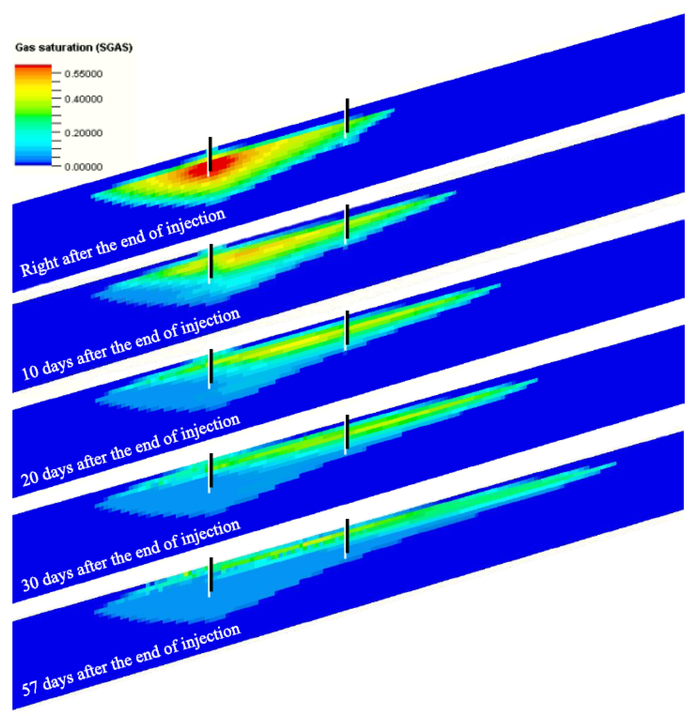
3.1. History Matching of the Well Pressure for Frio Project

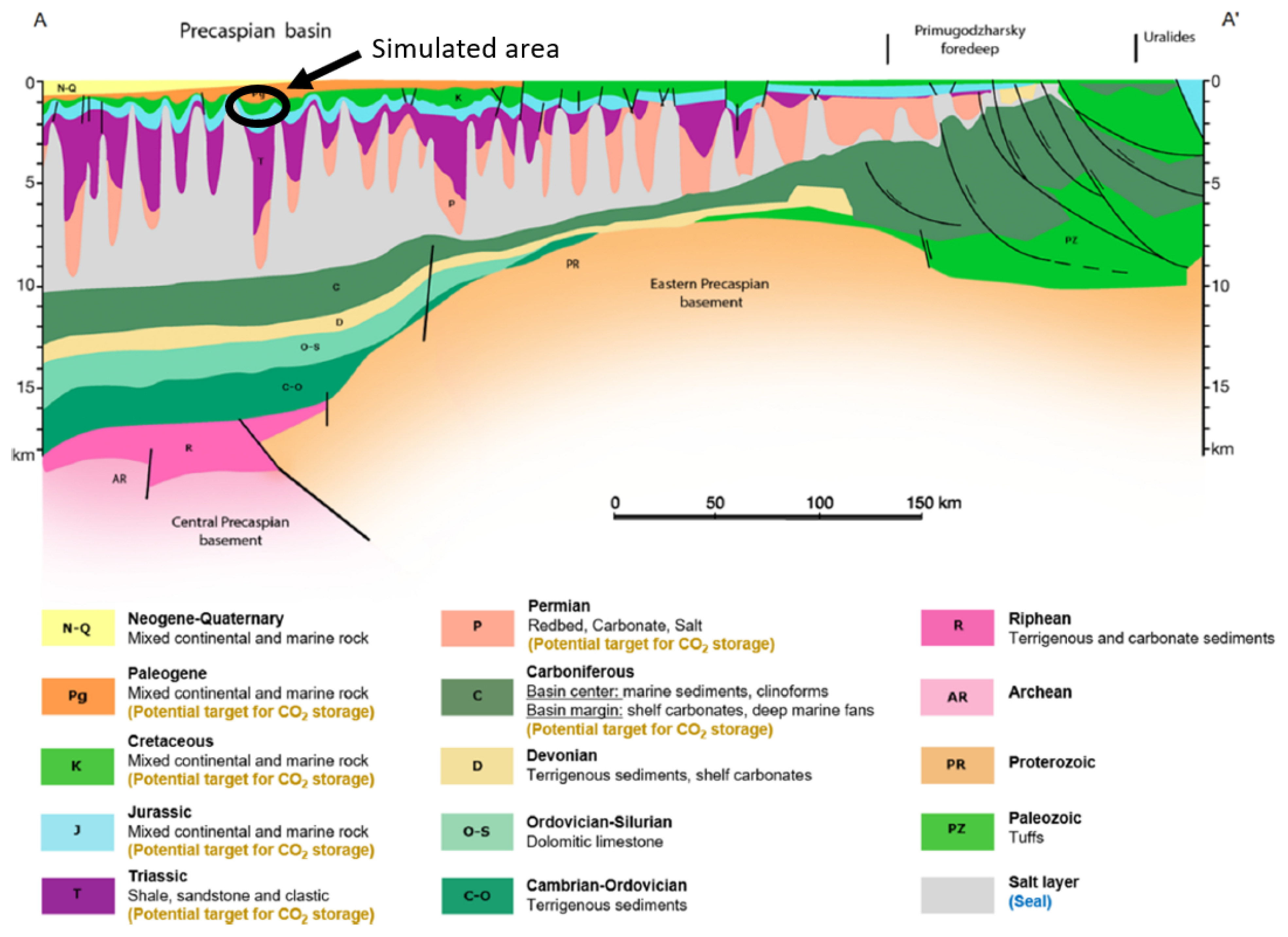
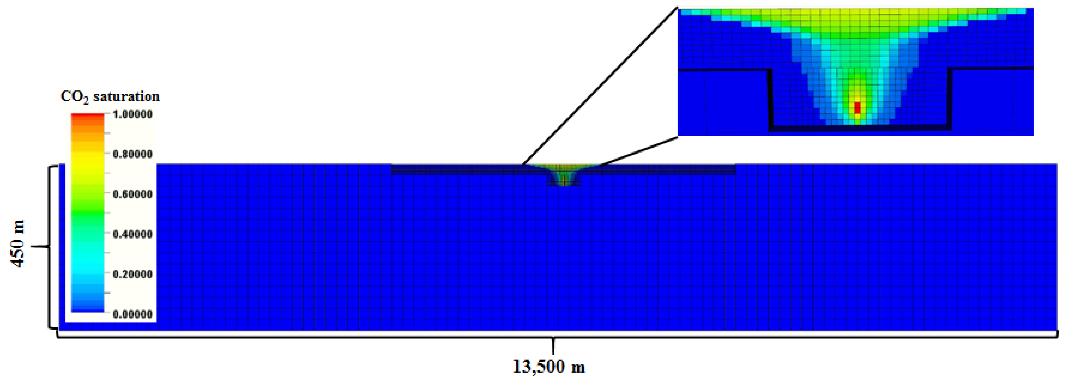
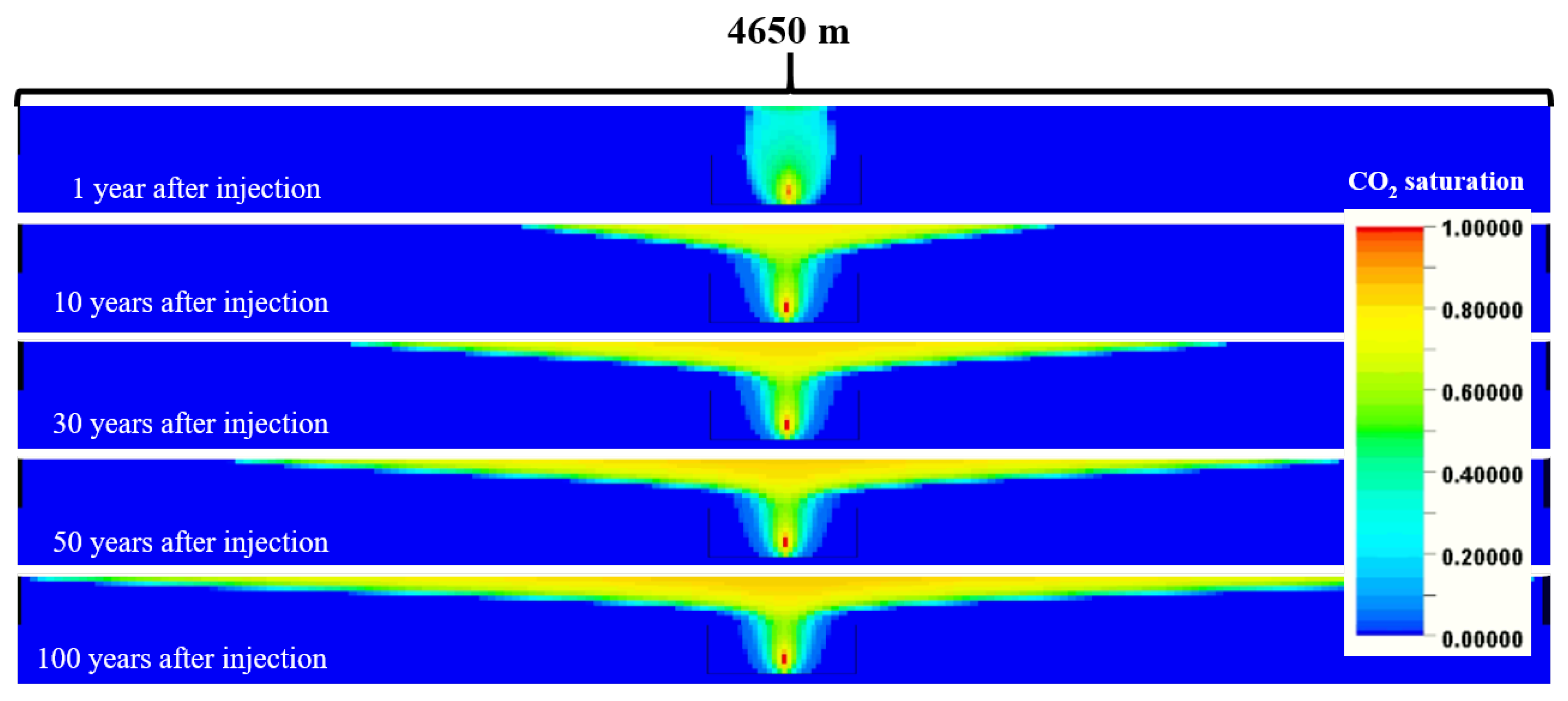
The initial grid for the reservoir simulation of Frio project was set as a square with equal sides of 2250 m (150 cells in each direction with lateral width of 15 m) for the x-y directions (see Figure 6). Another option tried was to shorten the width of the model to 855 m (see Figure 7).

We should note that based on the Frio field geological model in [9,19], there are no-flow boundary conditions from three sides of the reservoir (salt dome from one side and two main faults from the remaining two sides). To improve history matching, we tested different values of pore volume multiplier for the remaining side.

As observed from Figure 8, the width of the reservoir seems to be ambiguous, as when the width of the reservoir is shortened to 855 m (Figure 7), the BHP (bottom-hole pressure) of injector started to deviate from the historically recorded pressure, which was also observed in [22]. It seems that the width should be larger than the width based on the geological model, and the deviation of BHP is shown in Figure 8. The distance from the one of boundaries to the injector in the rectangle model is closer than in the square model (see Figure 6 and Figure 7). Pressure disturbance achieves the closest side boundary earlier in the rectangle model and affects well pressures. The alternative option was tested by placing wells in the center of the grid and retaining the width of 855 meters (see for more details Figure 9). In that case, we can obesrve that well pressure is less affected by the closest boundary as the wells are now situated in the center of the grid. However, we still observe the deviation of the simulated well pressure from the historical BHP (Figure 8). In order to achieve history matching on injector’s BHP and to receive a consistent CO${}_2$ plume shape with width = 2250 m, the different parameters were varied, which are discussed below.

Due to the uncertainty of permeability in the reservoir, we conducted numerical experiments for the vertical to horizontal permeability ratio (kv/kh) from 0.01 to 0.1. We should note that the vertical direction of CO${}_2$ plume flowing towards the reservoir top can be impacted by this ratio. The various numerical experiments demonstrated a small impact of kv/kh variation on injector’s BHP. Finally, the value of 0.1 was kept as a base case because it is commonly used in the industry [23] to account for vertical flow restrictions.

The horizontal permeability far from the injection well trajectory was a key parameter for variation in order to match the injector’s observed BHP and CO${}_2$ plume migration. The simulations indicate that the value of BHP increased when the value of horizontal permeability decreased. Moreover, this slows down horizontal migration of CO${}_2$ plume from the injector towards the producer. The horizontal permeability in x and y directions was multiplied by 0.5 outside the injection well (but not for cells perforated by well, because the data in the well area are measured and known) in order to obtain a history match on injection well flowing BHP. The alternative option is the change of productivity index (PI) of the well instead of changing horizontal permeability. However, the PI application will impact the perforated cells, which should be untouched because permeability was taken directly from the measured permeability curve. Critical gas saturation was one of the main parameters that had to historically match with CO${}_2$ plume migration, as it can impact the movement of gas and the amount of gas left as residual saturation. The values of this parameter such as 0, 1%, 5%, 10% and 20% were tested by using end point scaling (three-point scaling) in order to achieve a comparable CO${}_2$ plume to that of the conducted seismic survey from [24]. The value of 5% was chosen as the best one to match available data.

The pore volume multiplier on the edge cells of the model was the second most influential parameter on injectors’ BHP trend. The application of pore volume multiplier made the BHP trend consistent with the observed BHP trend. Its value of 1000 was chosen based on the iteration process to obtain a BHP trend consistent with an observed one. The multiplier was applied only to edge cells at the opposite side of the salt dome.

As shown in Figure 8, we achieved excellent matching between measured BHP (red dots) and modeled BHP (black line). It is important to note that the history match was improved by utilizing a width of 2250 m.

The CO${}_2$ plume from the history-matched reservoir simulation of the current study at different days is shown in Figure 10. The results are similar to CO${}_2$ plume migration from Figure 7 of [22].

3.2. Application of the CO${}_2$ Storage Model Using Data from Kazakhstan

Kazakhstan has many sedimentary basins or formations that can be used for potential CO${}_2$ storage [13]. The largest basin among them is the Precaspian basin, which has huge storage capacities compared to other basins, and it was chosen for modelling to show CO${}_2$ storage efficiency using a compositional flow simulation. In reservoir modeling, we consider a region of the postsalt formation, which is a good target for CO${}_2$ sequestration with the good reservoir characteristics where porosity is higher than 20% and permeability varies from 30 mD to several hundred millidarcies [13] with a presence of a good cap rock. As shown in Figure 11, the proposed region is located in a Cretaceous reservoir at depths of approximately 1000–2000 m. As its depth is more than 800 m, hydrostatic pressure is above 7.4 MPa, and the temperature is above 31 ${}^{\circ }$C, CO${}_2$ should be in a supercritical state in which the storage capacity is maximized. Another advantage of the proposed region is from economic point of view as the potential cost for drilling a new well is lower with lower formation depths.

In our model, the width and height of the region were set at 14 km and 450 m, respectively. A constant porosity value of 20% and a permeability value of 100 mD were taken as input for the reservoir model. As there was no SCAL (special core analysis) data available, the Frio field’s relative permeability and capillary pressure curves were taken as the basis for building the Precaspian model. The curves were taken only as a starting point; therefore, the study was performed to investigate the uncertainty of curves and their impact on the trapped amount of carbon dioxide. All other settings of the model are presented in

Table 1. Settings for the Precaspian model.

Parameter	Value
Depth of reservoir top, m	1073
Top perforation depth, m	1121
Pore pressure at reservoir top depth, bar	109
Overburden pressure at 1073 m and 1121 m, bar	232, 242
Reservoir temperature, C	55.7
Porosity, %	20
Horizontal permeability, mD	115
Kv/Kh ratio	0.1
Number of cells in I and J directions	90
Number of layers	15
Cell dimensions in I and J directions, m	150
Layer thickness, m	30
Injection rate, tons/day	223
Injection period, years	100
Post injection period, years	130
Total amount injected, millon tons	8.14

.

Similarly to the Frio model, local grid refinement around the injector was used for the the Precaspian basin model in order to achieve a good resolution and accurate movement of CO${}_2$ plume (see Figure 12).

Using a digitization tool, the depth of the reservoir top was taken as 1073 m (see Figure 11). The pore pressure of 109 bar at that depth was calculated by the hydrostatic formula by using a brine density of 1035 kg/m${}^3$. The reservoir temperature was taken as homogeneous in the reservoir, i.e., constant of 55.7 ${}^{\circ }$C. It was calculated by assuming an ambient surface temperature of 20 ${}^{\circ }$C and average geothermal gradient of 27.5 ${}^{\circ }$C/km. The gas injection rate was set at 120,000 m${}^3$/day (223 tons/day). This value is approximately equal to the injection rate in the Frio CO${}_2$ project. The consideration of fracture pressure should be taken into account while injecting CO${}_2$ into the Precaspian basin in order to avoid a generation of fractures around the well, which can act as a potential path for CO${}_2$ migration upwards to the surface. For several years, a great effort has been devoted to study of the properties of the fractured system such as pressure, geometry and other factors [25,26]. Fracture pressure was assumed at 65% from overburden pressure. Sixty-five percent of overburden pressure is potentially the minimum fracture pressure in the reservoir, but it can be higher than this value, achieving the overburden pressure itself. As Cretaceous formations mostly comprise clastic rocks, the average rock density was taken as 2200 kg/m${}^3$. The approximate overburden pressure at perforation depth of 1121 m is about 242 bar; hence, the minimum fracture pressure is 157 bar. In other words, the bottomhole pressure of injector should not increase the pressure of 157 bar.

The amount of trapped CO${}_2$, which includes dissolved CO${}_2$ in water, immobile residual CO${}_2$ and remaining amount of CO${}_2$ in mobile gas phase, was computed by using the reservoir model. The single realization homogeneous model with a constant porosity of 0.2 and permeability of 115 mD showed that after 100 years of injection, most of the CO${}_2$ was left in mobile phase, i.e., 80% of all injected CO${}_2$ (6.47 Mtons). Twelve percent of injected CO${}_2$ was dissolved in water (0.97 Mtons), and 8% was trapped as residual gas (0.69 Mtons). The reason for such an amount of trapped residual CO${}_2$ is that the saturation table of CO${}_2$-water has only 5% of irreducible gas saturation. Here, it should be noted that residual CO${}_2$ saturation is one of the uncertain parameters and can be higher than 5%, which will definitely result in an increased amount of trapped gas by capillary forces.

The extent of the CO${}_2$ migration after 1, 10, 30, 50 and 100 years after its injection is shown on Figure 13.

In order to model the post injection migration, we show the possible effect of residual gas trapping within 130 years after the end of injection. After stopping CO${}_2$ injection, it continues to dissolve in water. The amount of dissolved CO${}_2$ increased over time from 12% to 18% (1.43 Mtons), and the amount of CO${}_2$ trapped as residual gas increased from 8 to 10% (0.81 Mtons). The total of 28% of injected CO${}_2$ is trapped permanently, which is an indication of a good potential for CO${}_2$ storage. The remaining part of CO${}_2$ is in the mobile gas phase, but it also can be trapped by a sealed cap rock. To make it happen, the impermeable cap rock should exist. Moreover, injection pressure should be monitored in order to refrain from fracturing the cap rock. In addition, the spill points should also be monitored in order to prevent CO${}_2$ migration to other formations.

The uncertainty study was performed in order to observe how relative permeability taken from the Frio field and other most uncertain parameters (absolute permeability, porosity, residual CO${}_2$ saturation, critical water saturation, Corey gas and water coefficients) impact the trapped amount of CO${}_2$. The uncertainty range for permeability was taken as 30–200 mD [13]; for porosity it was taken as 10–30% (the porosity range was constrained between 10% and 30%, because the model is homogeneous and the average value should be over 20%); for residual gas saturation it was taken as 1–15%; for critical water saturation it was taken as 1–30%; for Corey gas coefficient it was taken as 1–3; and for Corey water coefficient it was taken as 1–5.

The uncertainty study included the following steps:

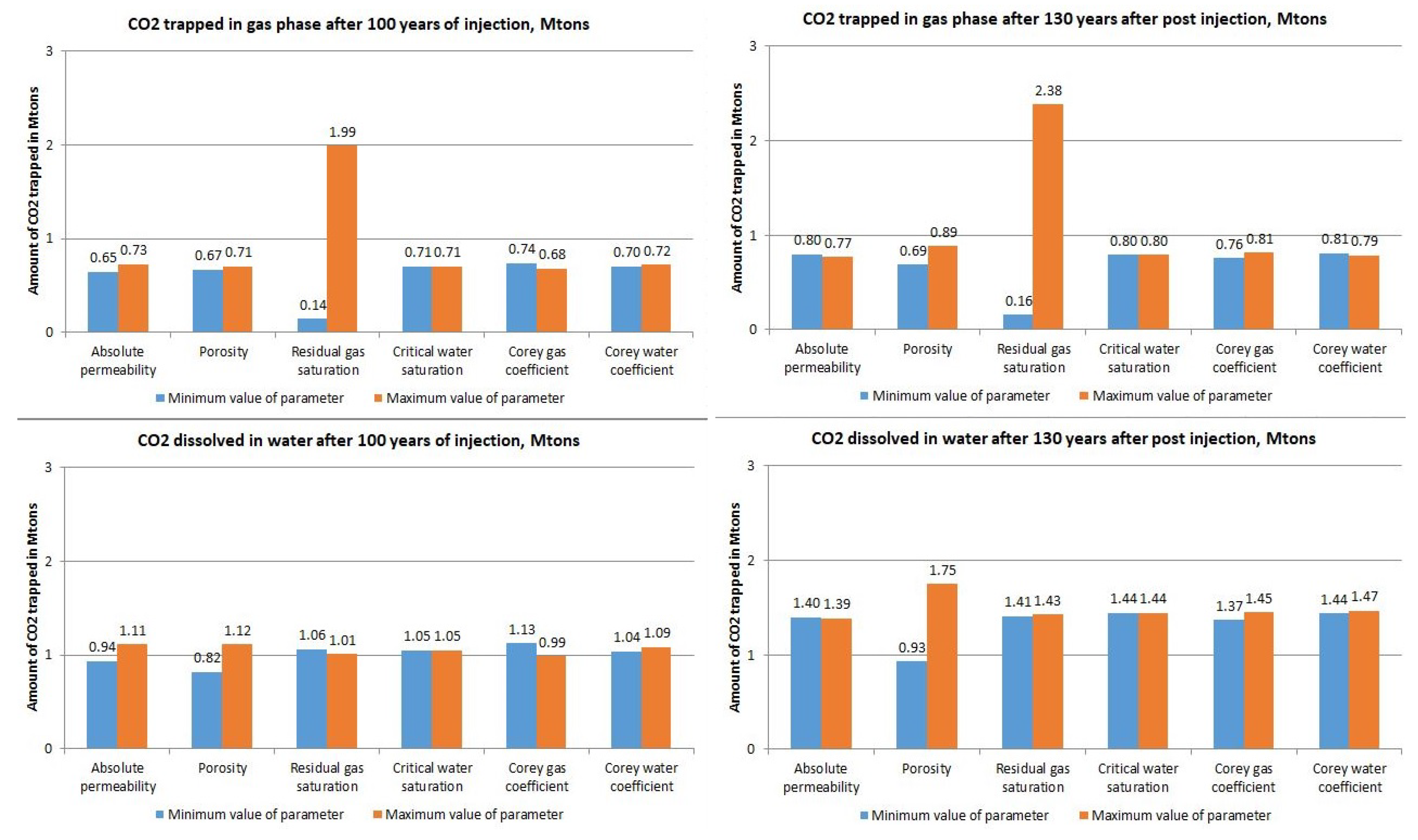
• Sensitivity analysis to determine how different parameters affect the trapped amount of CO${}_2$;
• Monte Carlo Latin Hypercube sampling method was used as experimental design in order to cover the entire range of uncertainty for six parameters;
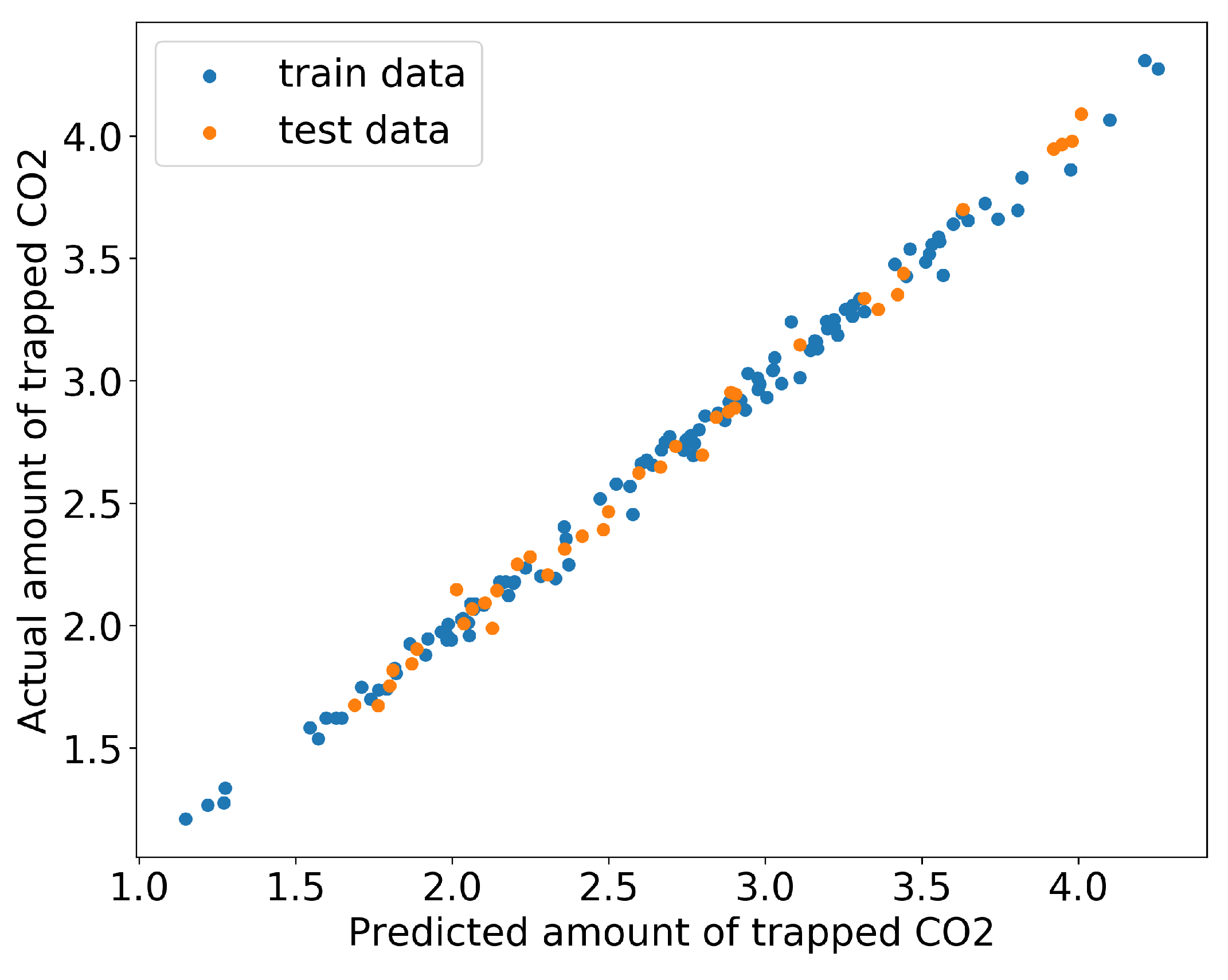
• The supervised learning algorithm was used to train the model using 75% of data taken from Monte Carlo simulation results;
• The trained model was used to explore the uncertainty range in more detail by generating an additional 10,000 cases;
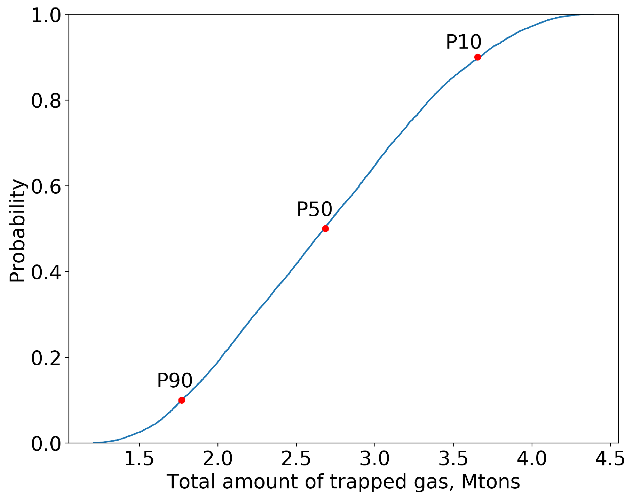
• The probability density function was built based on results of the Monte Carlo simulation and regression model, which gave us P10, P50 and P90 cases.

Firstly, sensitivity analysis on six uncertain parameters was performed to determine their impact on the trapped amount of CO${}_2$ using the OVAT (One-Variable-at-a-Time) technique when only one parameter was changed at a time (the value of parameter set to minimum and then to maximum; for absolute permeability, they are 30 mD and 200 mD; for porosity, they are 10 and 30%; for residual gas saturation, they are 1 and 15%; for critical water saturation, they are 1 and 30%; for Corey gas coefficient, they are 1 and 3; and for Corey water coefficient, they are 1 and 5) keeping all others at their original base values taken from a single realization homogeneous model (for absolute permeability, it is 115 mD; for porosity, it is 20%; for residual, gas saturation it is 5%; for critical water saturation, it is 15%; for Corey gas coefficient, it is 2; and for Corey water coefficient, it is 3). As observed from Figure 14, the trapped amount of CO${}_2$ in the gas phase is influenced mostly by residual gas saturation (the higher the residual gas saturation, the higher the amount of trapped CO${}_2$ in gas phase). The second most influential parameter here is porosity. Porosity is also a primary parameter that impacts the amount of CO${}_2$ dissolved in water mostly. Hence, the two most important and sensitive parameters are porosity and residual gas saturation. Other parameters have lower levels of impact. In addition, it should be mentioned that the only parameter that does not have any impact at all on the amount of trapped gas is critical (residual) water saturation.

Due to a limitation in computational power, we were able to run a small amount of cases. For this purpose, we used the Monte Carlo Latin Hypercube sampling method and generated 150 cases by mixing six most uncertain parameters. The Latin Hypercube sampling method is a good option when we need to cover evenly the entire area of uncertainty with a minimum number of samples [27]. The total injected CO${}_2$ was the same in all 150 cases.

The correlation between parameters and trapped amount of CO${}_2$ on Figure 15 shows that porosity strongly and positively correlates with the amount of CO${}_2$ dissolved in water and residual gas saturation with the amount of CO${}_2$ trapped in the gas phase as residual gas. The other four parameters (permeability, critical water saturation, Corey gas and water coefficients) do not correlate well with the amount of trapped CO${}_2$. These results from uncertainty analysis support the observations made during sensitivity analysis, which also confirms that the most influential parameters are porosity and residual CO${}_2$ saturation.

The last step was to use a machine learning tool to generate much more cases than we could create if using the reservoir simulator. The following supervised learning algorithms were tested for this purpose: random forest, linear regression and the second order polynomial regression model. Data consisting of 150 cases were divided randomly into two parts: 75% of data (e.g., using 112 cases out of 150 cases) for training the models and 25% of data (e.g., using 38 cases out of 150 cases) for testing the performance of models. All six uncertain parameters were used as input parameters for training models. The total amount of trapped CO${}_2$ (including dissolved amount of CO${}_2$ in water and trapped amount of CO${}_2$ in gas phase as residual gas) after 130 years after the post injection period was used as a target. The best algorithm was selected based on the following performance metrics: MAE (mean absolute error), MSE (mean squared error), RMST (root mean squared error) and coefficient of determination $R^2$ (Equations (4)–(7)):

$$MAE=\frac{1}{n}\sum _{j=1}^n|y_i-y_j|$$

(4)

where n is the total number of data points, $y_i$ is predicted value of target and $y_i$ is true value of target:

$$MSE=\frac{1}{n}\sum _{j=1}^n{|y_i-y_j|}^2$$

(5)

where n is the total number of data points, $y_i$ is predicted value of target and $y_i$ is true value of target:

$$MRST=\sqrt{\frac{1}{n}\sum _{j=1}^n{|y_i-y_j|}^2}$$

(6)

where n is the total number of data points, $y_i$ is predicted value of target and $y_i$ is true value of target:

$$R^2=1-\frac{S{S}_{res}}{S{S}_{tot}}=\frac{{\sum }_{j=1}^n(y_i-y_j)}{{\sum }_{j=1}^n(y_i-y_{mean})}$$

(7)

where n is the total number of data points, $y_i$ is predicted value of target, $y_i$ is true value of target, $y_{mean}$ is mean value of all true values of target, $S{S}_{res}$ is residual sum of squared errors and $S{S}_{tot}$ is total sum of squared errors.

As observed from

Table 2. Amount of CO${}_2$ after 130 years after the post injection period.

Algorithm	R2	MAE	MSE	MRST
Random forest	0.94	0.15	0.03	0.17
Linear regression	0.97	0.09	0.01	0.12
Second order polynomial regression	0.99	0.04	0.003	0.06

, the best algorithm was the second order polynomial regression model, which has the lowest MAE, MSE and RMST errors and the highest $R^2$. The performance metrics in Table 2 are calculated on the test data (25% of data which were not used for training the models, i.e., on 38 out of 150 cases) and train data(75%).

The polynomial regression model shows a very good prediction capability (see more details in Figure 16).

The cumulative density function is illustrated in Figure 17. P10, P50 and P90 values from the cumulative density function are as follows: 3.65 Mtons, 2.68 Mtons and 1.77 Mtons, respectively. Single realization homogeneous case (2.24 Mtons) lay between P90 and P50 values being closer to the P50 value.

We also should mention that the lower the injection point (the lower the perforations), the more contact area there is between CO${}_2$ and the formation water, which should result in improved trapping efficiency. The usage of horizontal injection wells should also increase the contact area between CO${}_2$ and the formation water; however, the drilling of such wells should be considered from an economic point of view as the drilling cost of such wells is more expensive.

4. Conclusions

In this paper, we used compositional flow simulation to model CO${}_2$ storage processes for the Frio CO${}_2$ project, USA, and a geological formation in the Precaspian basin, Kazakhstan. We obtained good history matching of the well pressure of the Frio project in the model. The impacts of different parameters on the model behavior were studied and analyzed with provided data. The result of CO${}_2$ migration in the Frio formation is consistent with other studies [22]. Next, we built a compositional flow model for a region of the Precapsian basin by using the relative permeability curves from the verified Frio field CO${}_2$ model.

An uncertainty study was performed to observe how relative permeability taken from the Frio field (end points as residual CO${}_2$ saturation and critical water saturation; and the shape of relative permeability curves as Corey gas and water coefficients) and the other two most uncertain parameters (absolute permeability and porosity) impacted the trapped amount of CO${}_2$. Sensitivity analysis showed that the most influential parameters are porosity and residual CO${}_2$ saturation. It was clear from the uncertainty study that the residual CO${}_2$ saturation has a strong positive correlation with the amount of CO${}_2$ trapped in the gas phase and that porosity has a strong positive correlation with the amount of CO${}_2$ dissolved in water. The overall study has shown that approximately 8.14 million tons of CO${}_2$ can be injected into the region of the Precaspian basin within 100 years with an injection rate of 223 tons/day. The period of 130 years of post injection showed that the total amount of trapped CO${}_2$ is about 2.68 Mtons (which is about 33 % of total injected CO${}_2$) based on the P50 case. The minimum amount of CO${}_2$, which is expected to be trapped, should be about 1.77 Mtons based on the P10 case. On the other hand, the results show that most of injected CO${}_2$ remains in mobile gaseous phases and can be trapped only by hydrodynamic trapping mechanisms due to having a good cap rock. The findings suggest that this approach could be useful for decision makers in considering a CO${}_2$ sequestration project in Kazakhstan.

References

1. Ringrose, P.S.; Meckel, T.A. Maturing global CO2 storage resources on offshore continental margins to achieve 2DS emissions reductions. Sci. Rep. 2019, 9, 1–10. [Google Scholar]
2. Aminu, M.D.; Nabavi, S.A.; Rochelle, C.A.; Manovic, V. A review of developments in carbon dioxide storage. Appl. Energy 2017, 208, 1389–1419. [Google Scholar] [CrossRef] [Green Version]
3. Min, B.; Sun, A.Y.; Wheeler, M.F.; Jeong, H. Utilization of Multiobjective Optimization for Pulse Testing Dataset from a CO2-EOR/Sequestration Field. J. Pet. Sci. Eng. 2018, 170, 244–266. [Google Scholar] [CrossRef]
4. Ringrose, P. How to Store CO2 Underground: Insights from Early-Mover CCS Projects; Springer: Berlin/Heidelberg, Germany, 2020. [Google Scholar]
5. Eigestad, G.T.; Dahle, H.K.; Hellevang, B.; Riis, F.; Johansen, W.T.; Øian, E. Geological modeling and simulation of CO2 injection in the Johansen formation. Comput. Geosci. 2009, 13, 435. [Google Scholar] [CrossRef]
6. Nilsen, H.M.; Lie, K.A.; Andersen, O. Analysis of CO2 trapping capacities and long-term migration for geological formations in the Norwegian North Sea using MRST-co2lab. Comput. Geosci. 2015, 79, 15–26. [Google Scholar] [CrossRef] [Green Version]
7. Delshad, M.; Kong, X.; Tavakoli, R.; Hosseini, S.A.; Wheeler, M.F. Modeling and simulation of carbon sequestration at Cranfield incorporating new physical models. Int. J. Greenh. Gas Control. 2013, 18, 463–473. [Google Scholar] [CrossRef]
8. Lu, X.; Lotfollahi, M.; Ganis, B.; Min, B.; Wheeler, M.F. An integrated flow-geomechanical analysis of flue gas injection in cranfield. In Proceedings of the SPE Improved Oil Recovery Conference. Society of Petroleum Engineers, Tulsa, OK, USA, 14–18 April 2018. [Google Scholar]
9. Ghomian, Y.; Pope, G.A.; Sepehrnoori, K. Reservoir simulation of CO2 sequestration pilot in Frio brine formation, USA Gulf Coast. Energy 2008, 33, 1055–1067. [Google Scholar] [CrossRef]
10. Kerimray, A.; Suleimenov, B.; De Miglio, R.; Rojas-Solórzano, L.; Gallachóir, B.Ó. Long-term climate change mitigation in Kazakhstan in a post Paris agreement context. In Limiting Global Warming to Well Below 2 °C: Energy System Modelling and Policy Development; Springer: Berlin/Heidelberg, Germany, 2018; pp. 297–314. [Google Scholar]
11. Heidug, W.; Lipponen, J.; McCoy, S.; Benoit, P. Storing CO2 through Enhanced Oil Recovery: Combining EOR with CO2 Storage (EOR+) for Profit; IEA: Paris, France, 2015. [Google Scholar]
12. Nurseitova, D. Carbon capture and storage in geological formations: The potential for Kazakhstan 1. In Sustainable Energy in Kazakhstan; Routledge: Milton, UK, 2017; pp. 134–143. [Google Scholar]
13. Abuov, Y.; Seisenbayev, N.; Lee, W. CO2 storage potential in sedimentary basins of Kazakhstan. Int. J. Greenh. Gas Control. 2020, 103, 103186. [Google Scholar] [CrossRef]
14. Hovorka, S.D.; Benson, S.M.; Doughty, C.; Freifeld, B.M.; Sakurai, S.; Daley, T.M.; Kharaka, Y.K.; Holtz, M.H.; Trautz, R.C.; Nance, H.S. Measuring permanence of CO2 storage in saline formations: The Frio experiment. Environ. Geosci. 2006, 13, 105–121. [Google Scholar] [CrossRef]
15. Spycher, N.; Pruess, K. CO2-H2O mixtures in the geological sequestration of CO2. II. Partitioning in chloride brines at 12–100 °C and up to 600 bar. Geochim. Cosmochim. Acta 2005, 69, 3309–3320. [Google Scholar] [CrossRef]
16. Amanbek, Y.; Singh, G.; Wheeler, M.F.; van Duijn, H. Adaptive numerical homogenization for upscaling single phase flow and transport. J. Comput. Phys. 2019, 387, 117–133. [Google Scholar] [CrossRef]
17. Amanbek, Y.; Singh, G.; Pencheva, G.; Wheeler, M.F. Error indicators for incompressible Darcy Flow problems using Enhanced Velocity Mixed Finite Element Method. Comput. Methods Appl. Mech. Eng. 2020, 363, 112884. [Google Scholar] [CrossRef] [Green Version]
18. Li, H.; Leung, W.T.; Wheeler, M.F. Sequential local mesh refinement solver with separate temporal and spatial adaptivity for non-linear two-phase flow problems. J. Comput. Phys. 2020, 403, 109074. [Google Scholar] [CrossRef] [Green Version]
19. Doughty, C.; Freifeld, B.M.; Trautz, R.C. Site characterization for CO2 geologic storage and vice versa: The Frio brine pilot, Texas, USA as a case study. Environ. Geol. 2008, 54, 1635–1656. [Google Scholar] [CrossRef]
20. Brooks, R.H.; Corey, A. Hydraulic Properties of Porous Media; Colorado State University: Fort Collins, CO, USA, 1964. [Google Scholar]
21. Skjaeveland, S.; Siqveland, L.; Kjosavik, A.; Hammervold, W.; Virnovsky, G. Capillary Pressure Correlation for Mixed-Wet Reservoirs. SPE Reserv. Eval. Eng. 2000, 3, 60–67. [Google Scholar] [CrossRef]
22. Jung, H.; Singh, G.; Espinoza, D.N.; Wheeler, M.F. Quantification of a maximum injection volume of CO2 to avert geomechanical perturbations using a compositional fluid flow reservoir simulator. Adv. Water Resour. 2018, 112, 160–169. [Google Scholar] [CrossRef]
23. Fanchi, J.R. 4-Porosity and Permeability. In Integrated Reservoir Asset Management; Fanchi, J.R., Ed.; Gulf Professional Publishing: Boston, MA, USA, 2010; pp. 49–69. [Google Scholar] [CrossRef]
24. Hovorka, S.D.; Sakurai, S.; Kharaka, Y.K.; Nance, H.S.; Doughty, C.; Benson, S.M.; Freifeld, B.M.; Trautz, R.C.; Phelps, T.; Daley, T.M. Monitoring CO2 Storage in Brine Formations: Lessons Learned from the Frio Field Test One Year Post Injection. 2006. Available online: https://www.beg.utexas.edu/gccc/bookshelf/Final%20Papers/06-06-Final.pdf (accessed on 6 March 2021).
25. Amanbek, Y.; Merembayev, T.; Srinivasan, S. Framework of Fracture Network Modeling using Conditioned Data with Sequential Gaussian Simulation. arXiv 2020, arXiv:2003.01327. [Google Scholar]
26. Almani, T.; Kumar, K.; Singh, G.; Wheeler, M.F. Stability of multirate explicit coupling of geomechanics with flow in a poroelastic medium. Comput. Math. Appl. 2019, 78, 2682–2699. [Google Scholar] [CrossRef]
27. Latin Hypercube Sampling. Wikipedia. 23 June 2021. Available online: https://en.wikipedia.org/wiki/Latin_hypercube_sampling (accessed on 16 August 2021).
Figure 1. Grid for Frio project.
Energies 14 08023 g001
Figure 2. Local grid refinement around wells: 1—injection well; 2—observation well.
Energies 14 08023 g002
Figure 3. The porosity and horizontal permeability curves from Frio field and averaged values per meter. (a) Porosity. (b) Permeability.
Energies 14 08023 g003
Figure 4. Relative permeability curves for CO 2 and water where S w = 0.15 . Corey function was fitted to drainage and imbibition relative permeability curves from [19]. (a) Drainage relative permeability curves, K R G -relative permeability of gas, K R W -relative permeability of water, Digitized-data from [19]. (b) Imbibition relative permeability curves, K R G -relative permeability of gas, K R W -relative permeability of water, Digitized-data from [19].
Energies 14 08023 g004
Figure 5. Corey function was fitted to drainage and imbibition capillary pressure curves from [19]. (a) Drainage capillary pressure. (b) Imbibition capillary pressure.
Energies 14 08023 g005
Figure 6. Square model with a length and width of 2250 m.
Energies 14 08023 g006
Figure 7. Rectangle model with a width of 855 m and length of 2250 m.
Energies 14 08023 g007
Figure 8. History match of injector’s BHP. BHP for model with width = 2250 m (black line), model with width = 855 m (blue line), model with width = 855 m and wells placed in the center of the grid (green line). Length of the models = 2250 in all 3 cases.
Energies 14 08023 g008
Figure 9. Rectangle model with a width of 855 m and length of 2250 m where the well is in the center.
Energies 14 08023 g009
Figure 10. CO 2 plume migration for the Frio project based on the history-matched simulation model.
Energies 14 08023 g010
Figure 11. Potential reservoirs for CO 2 storage in Precaspian basin adopted from [13].
Energies 14 08023 g011
Figure 12. Grid with local grid refinement in the center of the Precaspian model.
Energies 14 08023 g012
Figure 13. CO 2 migration in Precaspian model for 1, 10, 30, 50 and 100 years.
Energies 14 08023 g013
Figure 14. Sensitivity analysis on uncertain parameters and their impact on trapped amount of CO 2 during 100 years of injection and after 130 years of post injection.
Energies 14 08023 g014
Figure 15. Correlation between parameters and trapped amount of CO 2 at 130 years after the end of injection.
Energies 14 08023 g015
Figure 16. Correlation between predicted amount of trapped CO 2 by the second order polynomial regression and actual amount of trapped CO 2 simulated by reservoir simulator.
Energies 14 08023 g016
Figure 17. Cumulative density function for total amount of trapped CO 2 after 130 years after the end of injection.
Energies 14 08023 g017