
A Hybrid Optimization Algorithm for Solving of the Unit Commitment Problem Considering Uncertainty of the Load Demand

 ,
,  ,
,  ,
,  , and
, and 
Abstract
:1. Introduction
1.1. Unit Commitment
1.2. Literature Review
1.3. Contributions
- Solving the UCP under deterministic and probabilistic states. In a stochastic case, the uncertainty in the load side is considered.
- An efficient hybrid approach between modified particle swarm optimization and equilibrium optimizer (MPSO-EO) is proposed for solving the UCP.
- Validation the performance of the MPSO-EO through standard benchmark functions.
- A comparison between the proposed algorithm and well-known techniques such as EO, PSO, GWO and SCA for the solution of the UCP.
2. Problem Formulation
2.1. Objective Function
2.1.1. Fuel Cost
2.1.2. Start-Up Cost
2.1.3. Shutdown Cost
2.2. Constraints
2.2.1. Thermal Units Constraints
- (a)
- Generation power limits
- (b)
- Minimum up/down time constraints
- Minimum up time constraint
- Minimum down time constraint
- (c)
- Spinning reserve
2.2.2. System Constraints
- (a)
- Power balance constraint
2.3. Load Uncertainty Model
3. Optimization Algorithm
3.1. Particle Swarm Optimization (PSO)
3.2. Equilibrium Optimizer (EO)
3.2.1. Initialization
3.2.2. Equilibrium Candidates and Equilibrium Pool
3.2.3. Exponential Term and Concentrations Update
3.2.4. Generation Rate and Concentrations Update
3.2.5. Memory Saving for Particles
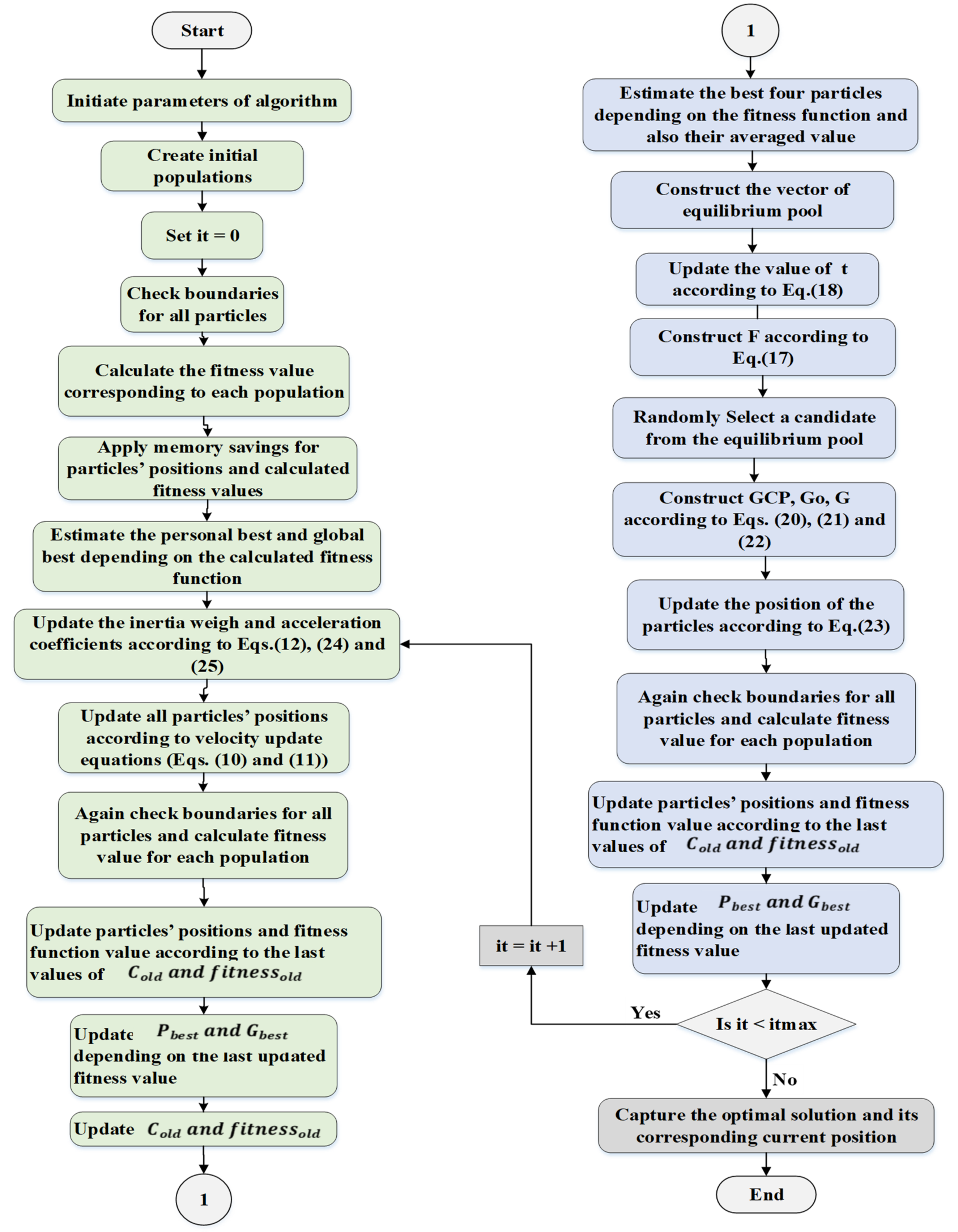
3.3. The Proposed Hybrid Methodology
4. Results and Discussion
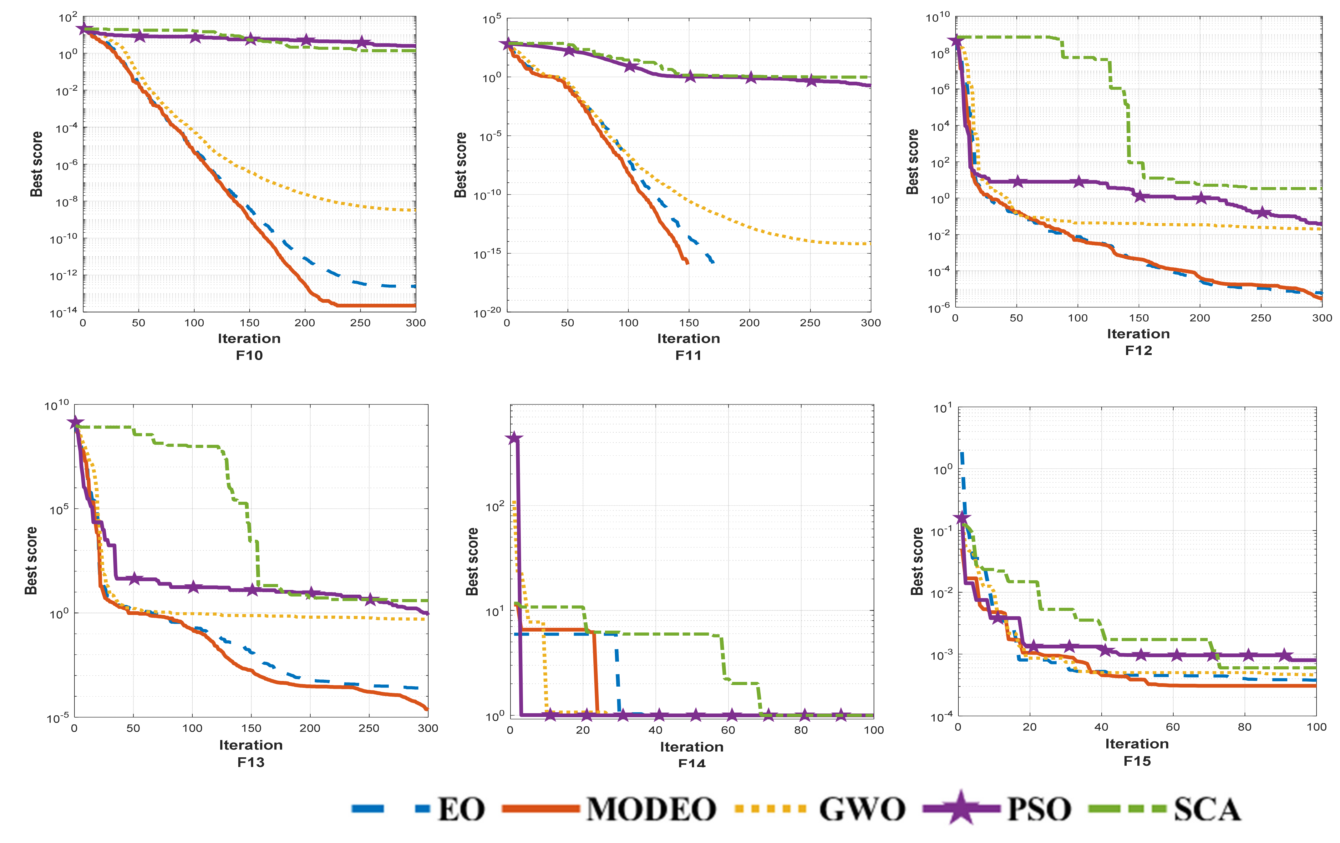
4.1. First: Application on Benchmark Test Functions
4.1.1. Benchmark Test Functions
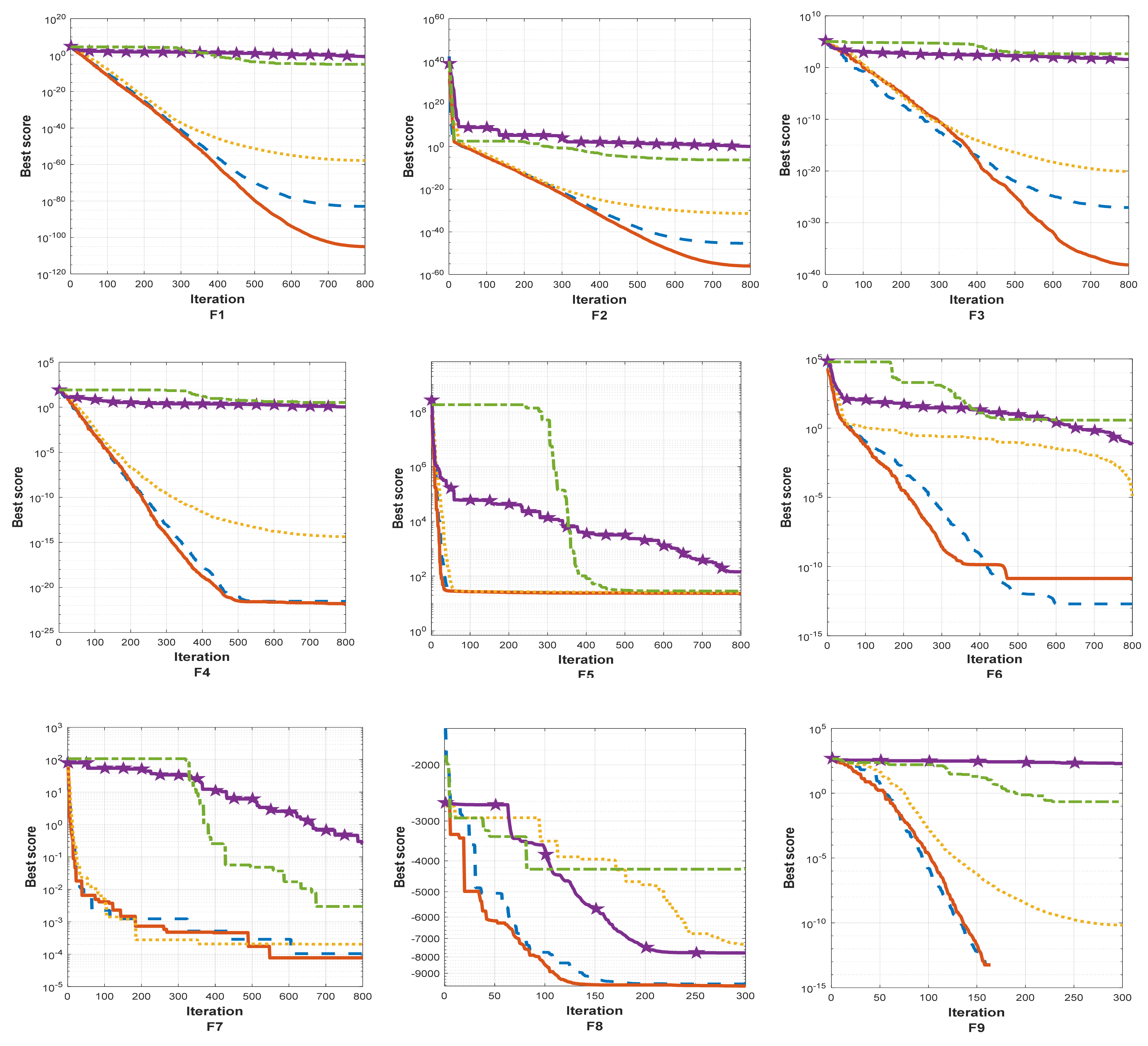
4.1.2. Benchmark Test Functions Comparison
4.2. Second: Application on the UCP
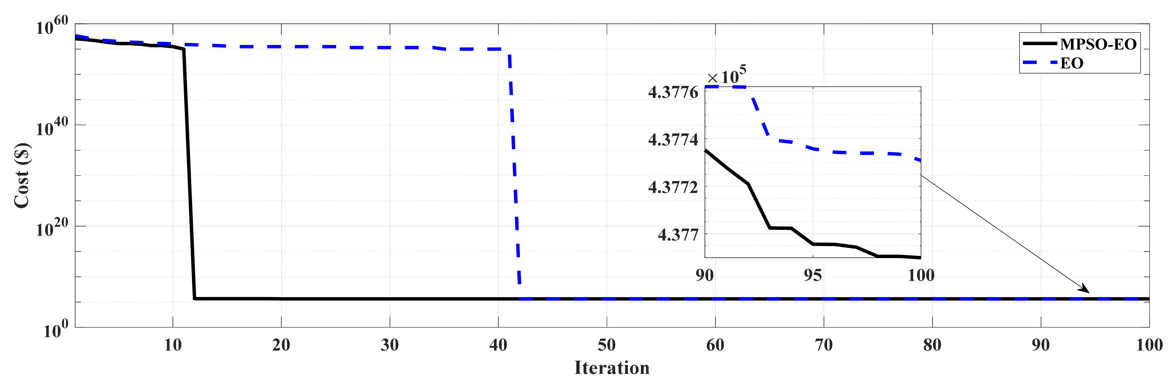
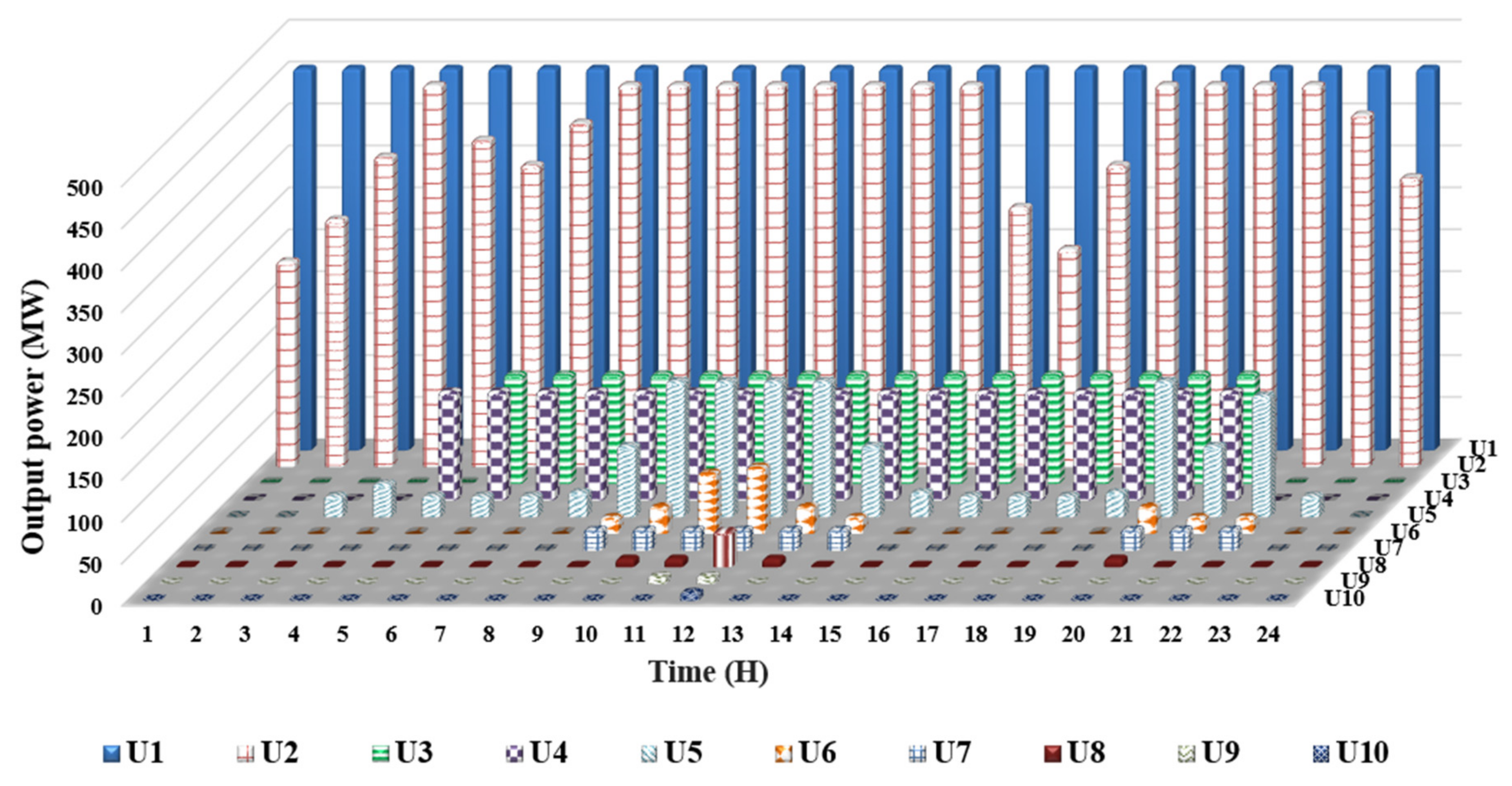
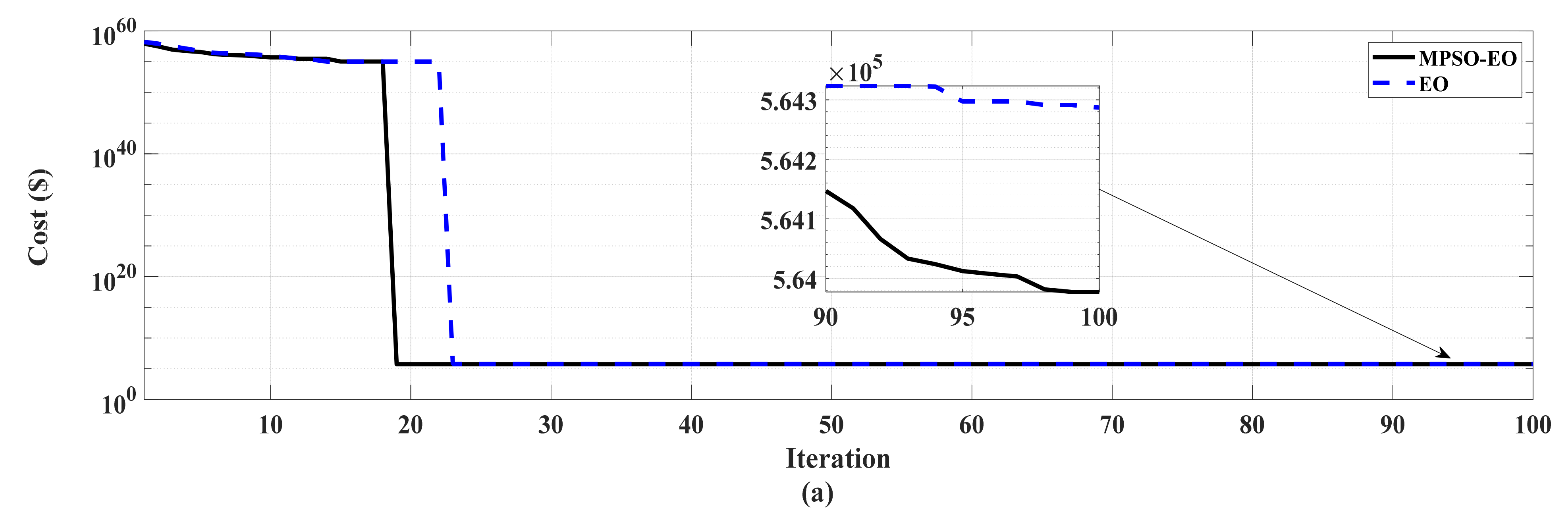
4.2.1. Performance of MPSO-EO for Test System 1
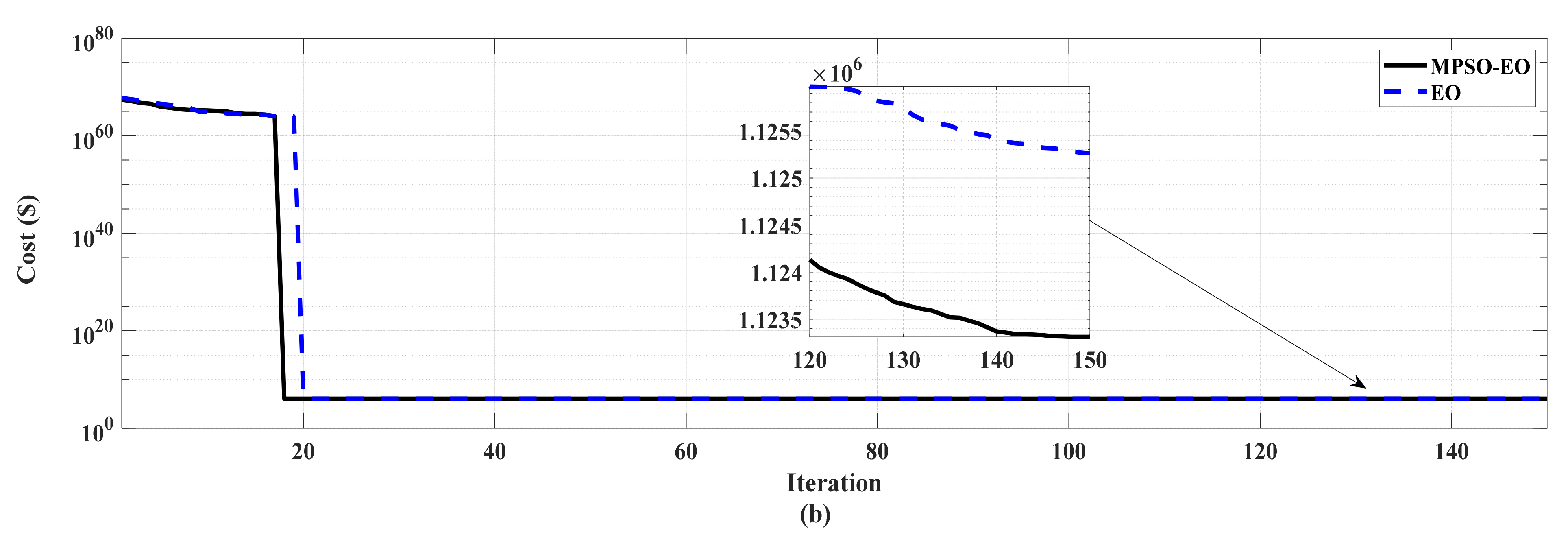
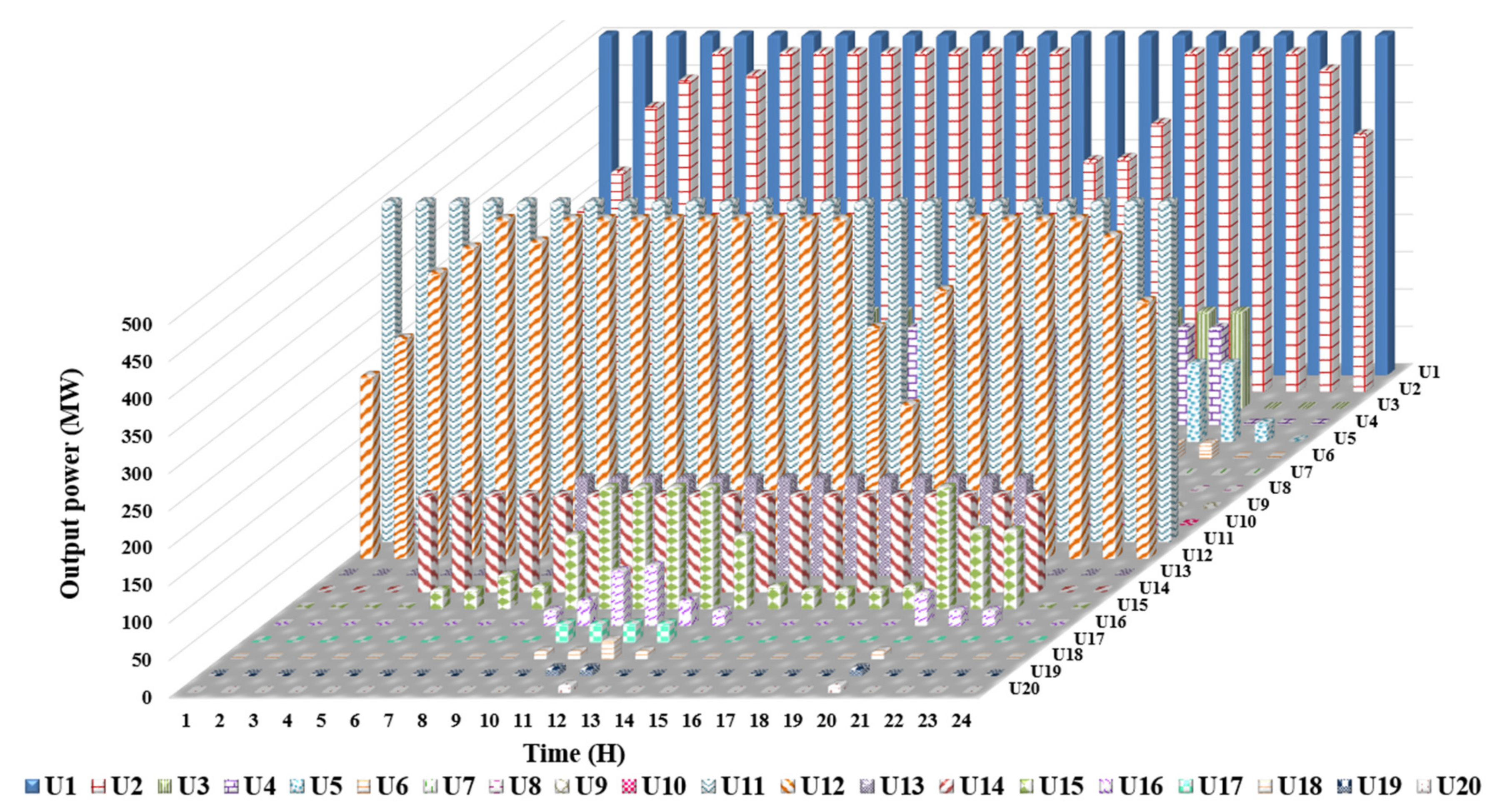
4.2.2. Performance of MPSO-EO for Test System 2
5. Conclusions
- Solving the UCP with the integration of renewable energy sources and energy storage systems;
- Solving the stochastic UCP by considering uncertainty in both load and generation sides to have a more reliable solution.
Author Contributions
Funding
Institutional Review Board Statement
Informed Consent Statement
Data Availability Statement
Acknowledgments
Conflicts of Interest
Nomenclature
| t | Index of time horizon for a set of T |
| i | Index of thermal generating units for a set of N |
| Fuel cost function of thermal unit i at time t | |
| Start-up cost function of thermal unit i at time t | |
| Shutdown cost function of thermal unit i at time t | |
| Hot start-up cost of thermal unit i | |
| Cold start-up cost of thermal unit i | |
| Minimum up time of thermal unit i | |
| Minimum down time of thermal unit i | |
| Time period that unit i was continuously off | |
| Time period that unit i was continuously on | |
| Time period for cooling down of unit i | |
| Minimum generation limit of thermal unit i | |
| Maximum generation limit of thermal unit i | |
| Load demand of the system at time t | |
| Spinning reserve requirements of the system at time t | |
| Standard deviation of the load demand at time t | |
| Mean deviation of the load demand at time t | |
| Total operating cost (objective function) | |
| Output power of thermal unit i at time t | |
| On/off state of the thermal unit i at time t |
References
- Bhardwaj, A.; Tung, N.S.; Shukla, V.K.; Kamboj, V.K. The important impacts of unit commitment constraints in power system planning. Int. J. Emerg. Trends Eng. Dev. 2012, 5, 301–306. [Google Scholar]
- Burns, R. Optimization of priority lists for a unit commitment program. In Proceedings of the IEEE Power Engineering Society Summer Meeting, San Francisco, CA, USA, 20–25 July 1975. [Google Scholar]
- Zhu, J. Optimization of Power System Operation; John Wiley & Sons: New York, NY, USA, 2015. [Google Scholar]
- Ananth, D.; Vineela, K. A review of different optimisation techniques for solving single and multi-objective optimisation problem in power system and mostly unit commitment problem. Int. J. Ambient. Energy 2021, 42, 1676–1698. [Google Scholar] [CrossRef]
- Virmani, S.; Adrian, E.C.; Imhof, K.; Mukherjee, S. Implementation of a Lagrangian relaxation based unit commitment problem. IEEE Trans. Power Syst. 1989, 4, 1373–1380. [Google Scholar] [CrossRef]
- Ongsakul, W.; Petcharaks, N. Unit commitment by enhanced adaptive Lagrangian relaxation. IEEE Trans. Power Syst. 2004, 19, 620–628. [Google Scholar] [CrossRef]
- Bakirtzis, A.; Zoumas, C. Lambda of Lagrangian relaxation solution to unit commitment problem. IEE Proc.-Gener. Transm. Distrib. 2000, 147, 131–136. [Google Scholar] [CrossRef]
- Senjyu, T.; Shimabukuro, K.; Uezato, K.; Funabashi, T. A fast technique for unit commitment problem by extended priority list. IEEE Trans. Power Syst. 2003, 18, 882–888. [Google Scholar] [CrossRef]
- Tingfang, Y.; Ting, T. Methodological Priority List for Unit Commitment Problem. In Proceedings of the 2008 International Conference on Computer Science and Software Engineering, Washington, DC, USA, 12–14 December 2008; IEEE: Manhattan, NY, USA, 2008; pp. 176–179. [Google Scholar]
- Muckstadt, J.A.; Wilson, R.C. An application of mixed-integer programming duality to scheduling thermal generating systems. IEEE Trans. Power Appar. Syst. 1968, PAS-87, 1968–1978. [Google Scholar] [CrossRef]
- Su, C.-C.; Hsu, Y.-Y. Fuzzy dynamic programming: An application to unit commitment. IEEE Trans. Power Syst. 1991, 6, 1231–1237. [Google Scholar]
- Patra, S.; Goswami, S.; Goswami, B. Fuzzy and simulated annealing based dynamic programming for the unit commitment problem. Expert Syst. Appl. 2009, 36, 5081–5086. [Google Scholar] [CrossRef]
- Kazarlis, S.A.; Bakirtzis, A.; Petridis, V. A genetic algorithm solution to the unit commitment problem. IEEE Trans. Power Syst. 1996, 11, 83–92. [Google Scholar] [CrossRef]
- Swarup, K.; Yamashiro, S. Unit commitment solution methodology using genetic algorithm. IEEE Trans. Power Syst. 2002, 17, 87–91. [Google Scholar] [CrossRef]
- Zhao, B.; Guo, C.; Bai, B.; Cao, Y. An improved particle swarm optimization algorithm for unit commitment. Int. J. Electr. Power Energy Syst. 2006, 28, 482–490. [Google Scholar] [CrossRef]
- Pappala, V.S.; Erlich, I. A new approach for solving the unit commitment problem by adaptive particle swarm optimization. In Proceedings of the 2008 IEEE Power and Energy Society General Meeting-Conversion and Delivery of Electrical Energy in the 21st Century, Pittsburgh, PA, USA, 20–24 July 2008; IEEE: Manhattan, NY, USA, 2008; pp. 1–6. [Google Scholar]
- Roy, P.K. Solution of unit commitment problem using gravitational search algorithm. Int. J. Electr. Power Energy Syst. 2013, 53, 85–94. [Google Scholar] [CrossRef]
- Pan, J.-S.; Hu, P.; Chu, S.-C. Binary fish migration optimization for solving unit commitment. Energy 2021, 226, 120329. [Google Scholar] [CrossRef]
- Chandrasekaran, K.; Simon, S.P.; Padhy, N.P. Binary real coded firefly algorithm for solving unit commitment problem. Inf. Sci. 2013, 249, 67–84. [Google Scholar] [CrossRef]
- Mantawy, A.; Abdel-Magid, Y.L.; Selim, S.Z. A simulated annealing algorithm for unit commitment. IEEE Trans. Power Syst. 1998, 13, 197–204. [Google Scholar] [CrossRef]
- Venkatesh Kumar, C.; Ramesh Babu, M. An Exhaustive Solution of Power System Unit Commitment Problem Using Enhanced Binary Salp Swarm Optimization Algorithm. J. Electr. Eng. Technol. 2021, 1–19. [Google Scholar] [CrossRef]
- Rajan, C.C.A.; Mohan, M. An evolutionary programming-based tabu search method for solving the unit commitment problem. IEEE Trans. Power Syst. 2004, 19, 577–585. [Google Scholar] [CrossRef]
- Kamboj, V.K. A novel hybrid PSO–GWO approach for unit commitment problem. Neural Comput. Appl. 2016, 27, 1643–1655. [Google Scholar] [CrossRef]
- Bavafa, M.; Monsef, H.; Navidi, N. A new hybrid approach for unit commitment using lagrangian relaxation combined with evolutionary and quadratic programming. In Proceedings of the 2009 Asia-Pacific Power and Energy Engineering Conference, Wuhan, China, 28–31 March 2009; IEEE: Manhattan, NY, USA, 2009; pp. 1–6. [Google Scholar]
- Anand, H.; Narang, N.; Dhillon, J. Multi-objective combined heat and power unit commitment using particle swarm optimization. Energy 2019, 172, 794–807. [Google Scholar] [CrossRef]
- Trivedi, A.; Srinivasan, D.; Biswas, S.; Reindl, T. A genetic algorithm–differential evolution based hybrid framework: Case study on unit commitment scheduling problem. Inf. Sci. 2016, 354, 275–300. [Google Scholar] [CrossRef]
- Trivedi, A.; Srinivasan, D.; Biswas, S.; Reindl, T. Hybridizing genetic algorithm with differential evolution for solving the unit commitment scheduling problem. Swarm Evol. Comput. 2015, 23, 50–64. [Google Scholar] [CrossRef]
- Zobaa, A.F.; Aleem, S.A. Uncertainties in Modern Power Systems; Academic Press: Cambridge, MA, USA, 2020. [Google Scholar]
- Unit, S.E. Reducing Re-Offending by Ex-Prisoners; Social Exclusion Unit London: London, UK, 2002. [Google Scholar]
- Kennedy, J.; Eberhart, R. Particle swarm optimization. In Proceedings of the ICNN’95-International Conference on Neural Networks, Perth, Australia, 27 November–1 December 1995; IEEE: Manhattan, NY, USA, 1995; pp. 1942–1948. [Google Scholar]
- Khan, A.; Hizam, H.; Abdul-Wahab, N.I.; Othman, M.L. Solution of Optimal Power Flow Using Non-Dominated Sorting Multi Objective Based Hybrid Firefly and Particle Swarm Optimization Algorithm. Energies 2020, 13, 4265. [Google Scholar] [CrossRef]
- Riaz, M.; Hanif, A.; Hussain, S.J.; Memon, M.I.; Ali, M.U.; Zafar, A. An optimization-based strategy for solving optimal power flow problems in a power system integrated with stochastic solar and wind power energy. Appl. Sci. 2021, 11, 6883. [Google Scholar] [CrossRef]
- Faramarzi, A.; Heidarinejad, M.; Stephens, B.; Mirjalili, S. Equilibrium optimizer: A novel optimization algorithm. Knowl.-Based Syst. 2020, 191, 105190. [Google Scholar] [CrossRef]
- Zellagui, M.; Lasmari, A.; Settoul, S.; El-Sehiemy, R.A.; El-Bayeh, C.Z.; Chenni, R. Simultaneous allocation of photovoltaic DG and DSTATCOM for techno-economic and environmental benefits in electrical distribution systems at different loading conditions using novel hybrid optimization algorithms. Int. Trans. Electr. Energy Syst. 2021, 31, e12992. [Google Scholar] [CrossRef]
- Anita, J.M.; Raglend, I.J. Solution of unit commitment problem using shuffled frog leaping algorithm. In Proceedings of the 2012 International Conference on Computing, Electronics and Electrical Technologies (ICCEET), Nagercoil, India, 21–22 March 2012; IEEE: Manhattan, NY, USA, 2012; pp. 109–115. [Google Scholar]
- Juste, K.; Kita, H.; Tanaka, E.; Hasegawa, J. An evolutionary programming solution to the unit commitment problem. IEEE Trans. Power Syst. 1999, 14, 1452–1459. [Google Scholar] [CrossRef]
- Simopoulos, D.N.; Kavatza, S.D.; Vournas, C.D. Unit commitment by an enhanced simulated annealing algorithm. IEEE Trans. Power Syst. 2006, 21, 68–76. [Google Scholar] [CrossRef]
- Saravanan, B.; Vasudevan, E.; Kothari, D. Unit commitment problem solution using invasive weed optimization algorithm. Int. J. Electr. Power Energy Syst. 2014, 55, 21–28. [Google Scholar] [CrossRef]
- Damousis, I.G.; Bakirtzis, A.G.; Dokopoulos, P.S. A solution to the unit-commitment problem using integer-coded genetic algorithm. IEEE Trans. Power Syst. 2004, 19, 1165–1172. [Google Scholar] [CrossRef]
- Viana, A.; de Sousa, J.P.; Matos, M. Using GRASP to solve the unit commitment problem. Ann. Oper. Res. 2003, 120, 117–132. [Google Scholar] [CrossRef]
- Jeong, Y.-W.; Park, J.-B.; Shin, J.-R.; Lee, K.Y. A thermal unit commitment approach using an improved quantum evolutionary algorithm. Electr. Power Compon. Syst. 2009, 37, 770–786. [Google Scholar] [CrossRef]
- Yuan, X.; Nie, H.; Su, A.; Wang, L.; Yuan, Y. An improved binary particle swarm optimization for unit commitment problem. Expert Syst. Appl. 2009, 36, 8049–8055. [Google Scholar] [CrossRef]
- Lau, T.; Chung, C.; Wong, K.; Chung, T.; Ho, S.L. Quantum-inspired evolutionary algorithm approach for unit commitment. IEEE Trans. Power Syst. 2009, 24, 1503–1512. [Google Scholar] [CrossRef]
- Panwar, L.K.; Reddy, S.; Verma, A.; Panigrahi, B.K.; Kumar, R. Binary grey wolf optimizer for large scale unit commitment problem. Swarm Evol. Comput. 2018, 38, 251–266. [Google Scholar] [CrossRef]
- Saravanan, B.; Mishra, S.; Nag, D. A solution to stochastic unit commitment problem for a wind-thermal system coordination. Front. Energy 2014, 8, 192–200. [Google Scholar] [CrossRef]
- Micev, M.; Ćalasan, M.; Ali, Z.M.; Hasanien, H.M.; Abdel Aleem, S.H.E. Optimal design of automatic voltage regulation controller using hybrid simulated annealing—Manta ray foraging optimization algorithm. Ain Shams Eng. J. 2021, 12, 641–657. [Google Scholar] [CrossRef]
- Refaat, M.M.; Aleem, S.H.E.; Atia, Y.; Ali, Z.M.; El-Shahat, A.; Sayed, M.M. A Mathematical Approach to Simultaneously Plan Generation and Transmission Expansion Based on Fault Current Limiters and Reliability Constraints. Mathematics 2021, 9, 2771. [Google Scholar] [CrossRef]
- Zobaa, A.F.; Aleem, S.H.E.A.; Abdelaziz, A.Y. Classical and Recent Aspects of Power System Optimization; Academic Press: Cambridge, MA, USA; Elsevier: Amsterdam, The Netherlands, 2018. [Google Scholar]


| Function No. | MPSO-EO | EO | PSO | GWO | SCA | |
|---|---|---|---|---|---|---|
| F1 | Best | 9.0495 × 10−106 | 1.1579 × 10−83 | 0.1215795 | 1.6997 × 10−58 | 9.3414 × 10⁻⁶ |
| Worst | 3.1214 × 10−100 | 4.2725 × 10−79 | 1.531071 | 6.1888 × 10−55 | 3.765 | |
| Mean | 1.573 × 10−101 | 4.3309 × 10−80 | 0.4307582 | 7.1958 × 10−56 | 0.1748 | |
| Std | 5.7719 × 10−101 | 9.83229 × 10−80 | 0.2737527 | 1.3523 × 10−55 | 0.6923 | |
| F2 | Best | 3.6375 × 10−56 | 6.6036 × 10−46 | 0.7375 | 1.3512 × 10⁻³² | 2.9791 × 10⁻⁶ |
| Worst | 3.4786 × 10−54 | 1.1718 × 10−43 | 41.2712 | 1.009 × 10⁻³⁰ | 0.00096 | |
| Mean | 4.2934 × 10−55 | 2.4282 × 10−44 | 4.8417 | 2.2264 × 10⁻³¹ | 0.00019 | |
| Std | 7.2358 × 10−55 | 2.9957 × 10−44 | 7.4781 | 2.389 × 10⁻³¹ | 0.0002 | |
| F3 | Best | 3.558 × 10−38 | 1.1168 × 10⁻²⁷ | 33.78574 | 1.7032 × 10⁻²⁰ | 17.18137 |
| Worst | 1.7073 × 10⁻²⁶ | 5.8834 × 10⁻²⁰ | 112.7994 | 8.5859 × 10⁻¹⁴ | 7716.624 | |
| Mean | 5.7827 × 10⁻²⁸ | 2.9493 × 10⁻²¹ | 65.95589 | 4.1645 × 10⁻¹⁵ | 2545.905 | |
| Std | 3.1155 × 10⁻²⁷ | 1.0939 × 10⁻²⁰ | 21.51473 | 1.5601 × 10⁻¹⁴ | 1954.96 | |
| F4 | Best | 8.9129 × 10⁻²³ | 1.0421 × 10⁻²² | 1.0515 | 1.8572 × 10⁻¹⁵ | 4.7894 |
| Worst | 3.0663 × 10⁻¹⁶ | 1.1162 × 10⁻¹⁹ | 1.8308 | 6.9359 × 10⁻¹³ | 46.8004 | |
| Mean | 2.9137 × 10⁻¹⁷ | 1.3109 × 10⁻²⁰ | 1.4866 | 8.9864 × 10⁻¹⁴ | 18.5352 | |
| Std | 6.3935 × 10⁻¹⁷ | 2.8049 × 10⁻²⁰ | 0.2206 | 1.333 × 10⁻¹³ | 10.9167 | |
| F5 | Best | 23.1873 | 23.8427 | 139.5195 | 24.9101 | 28.3771 |
| Worst | 24.2688 | 24.5458 | 1110.277 | 27.9375 | 10,848.22 | |
| Mean | 23.6952 | 24.1897 | 342.3329 | 26.40021 | 689.1504 | |
| Std | 0.29534 | 0.1921 | 211.188 | 0.7468 | 1999.06 | |
| F6 | Best | 1.3896 × 10⁻¹¹ | 2.0002 × 10⁻¹³ | 0.0669 | 1.2974 × 10⁻⁵ | 3.7721 |
| Worst | 7.1921 × 10⁻⁹ | 6.1705 × 10⁻¹⁰ | 0.8661 | 1.0023 | 5.5307 | |
| Mean | 8.3805 × 10⁻¹⁰ | 3.686 × 10⁻¹¹ | 0.3458 | 0.4026 | 4.4089 | |
| Std | 1.3708 × 10⁻⁹ | 1.1153 × 10⁻¹⁰ | 0.2197 | 0.2869 | 0.4089 | |
| F7 | Best | 7.6647 × 10⁻⁵ | 0.0001 | 0.2622 | 0.0002 | 0.0029 |
| Worst | 0.0005 | 0.00097 | 21.6872 | 0.0019 | 0.1073 | |
| Mean | 0.0003 | 0.00046 | 5.2364 | 0.0008 | 0.0285 | |
| Std | 0.0001 | 0.00019 | 5.8439 | 0.0004 | 0.0254 | |
| F8 | Best | −9865.201 | −9719.074 | −7770.439 | −7315.422 | −4246.805 |
| Worst | −7414.904 | −6908.452 | −2747.769 | −3016.587 | −3119.04 | |
| Mean | −8589.561 | −8503.638 | −5479.792 | −5846.141 | −3616.961 | |
| Std | 712.506 | 719.2974 | 1361.11 | 1328.698 | 283.2907 | |
| F9 | Best | 0 | 0 | 163.1299 | 5.5707 × 10⁻¹² | 21.3267 |
| Worst | 5.6843 × 10⁻¹⁴ | 2.2737 × 10⁻¹³ | 307.7645 | 20.5118 | 180.1624 | |
| Mean | 4.5474 × 10⁻¹⁵ | 2.9559 × 10⁻¹⁴ | 243.6789 | 6.4631 | 70.2827 | |
| Std | 1.5739 × 10⁻¹⁴ | 5.2201 × 10⁻¹⁴ | 38.1449 | 4.8576 | 33.9405 | |
| F10 | Best | 2.2204 × 10⁻¹⁴ | 2.4603 × 10⁻¹³ | 2.4881 | 3.2538 × 10⁻⁹ | 1.3701 |
| Worst | 5.7732 × 10⁻¹⁴ | 3.2623 × 10⁻¹² | 4.237 | 2.7796 × 10⁻⁸ | 20.4224 | |
| Mean | 3.4852 × 10⁻¹⁴ | 1.0424 × 10⁻¹² | 3.4253 | 1.1751 × 10⁻⁸ | 15.9039 | |
| Std | 7.7484 × 10⁻¹⁵ | 7.9499 × 10⁻¹³ | 0.4637 | 6.4636 × 10⁻⁹ | 7.5859 | |
| F11 | Best | 0 | 0 | 0.1689 | 6.3283 × 10⁻¹⁵ | 0.9503 |
| Worst | 0.0197 | 0.0246 | 0.6164 | 0.0296 | 9.5659 | |
| Mean | 0.0008 | 0.0042 | 0.3849 | 0.0087 | 2.1191 | |
| Std | 0.0039 | 0.0082 | 0.0847 | 0.0115 | 1.8833 | |
| F12 | Best | 2.7601 × 10⁻⁶ | 5.3834 × 10⁻⁶ | 0.0383 | 0.0201 | 3.3341 |
| Worst | 0.1039 | 0.1037 | 1.6209 | 0.1148 | 668,487 | |
| Mean | 0.0044 | 0.0042 | .3266 | 0.0547 | 344,523.6 | |
| Std | 0.02076 | 0.02073 | 0.3562 | 0.0273 | 134,615 | |
| F13 | Best | 2.1984 × 10⁻⁵ | 0.0002 | 0.7789 | 0.4995 | 3.8972 |
| Worst | 0.4761 | 0.4005 | 2.9736 | 1.2256 | 1.83 × 10⁷ | |
| Mean | 0.1437 | 0.081 | 1.5124 | 0.7896 | 134,352 | |
| Std | 0.15062 | 0.102 | 0.5359 | 0.1984 | 369,891 | |
| F14 | Best | 0.998 | 0.998 | 0.998 | 0.998 | 0.998 |
| Worst | 4.9505 | 2.9821 | 11.7187 | 15.5038 | 10.7631 | |
| Mean | 1.3945 | 1.5539 | 5.0092 | 5.8148 | 3.6726 | |
| Std | 0.9033 | 0.8142 | 3.1811 | 4.648 | 3.3029 | |
| F15 | Best | 0.00031 | 0.00037 | 0.0008 | 0.0005 | 0.0006 |
| Worst | 0.0204 | 0.02036 | 0.0203 | 0.0203 | 0.0025 | |
| Mean | 0.0013 | 0.0015 | 0.0068 | 0.0069 | 0.0015 | |
| Std | 0.0039 | 0.0039 | 0.0087 | 0.0094 | 0.0006 |
| Time | 1 | 2 | 3 | 4 | 5 | 6 | 7 | 8 | 9 | 10 | 11 | 12 |
|---|---|---|---|---|---|---|---|---|---|---|---|---|
| Load demand | 700 | 750 | 850 | 950 | 1000 | 1100 | 1150 | 1200 | 1300 | 1400 | 1450 | 1500 |
| Reserve values | 70 | 75 | 85 | 95 | 100 | 110 | 115 | 120 | 130 | 140 | 145 | 150 |
| Time | 13 | 14 | 15 | 16 | 17 | 18 | 19 | 20 | 21 | 22 | 23 | 24 |
| Load demand | 1400 | 1300 | 1200 | 1050 | 1000 | 1100 | 1200 | 1400 | 1300 | 1100 | 900 | 800 |
| Reserve values | 140 | 130 | 120 | 105 | 100 | 110 | 120 | 140 | 130 | 110 | 90 | 80 |
| Unit | a ($/h) | b ($/MWh) | c h) | (MW) | (MW) | (h) | (h) | (h) | Initial State (h) | ||
|---|---|---|---|---|---|---|---|---|---|---|---|
| Un 1 | 1000 | 16.19 | 0.00048 | 455 | 150 | 4500 | 9000 | 8 | 8 | 5 | 8 |
| Un 2 | 970 | 17.26 | 0.00031 | 455 | 150 | 5000 | 10,000 | 8 | 8 | 5 | 8 |
| Un 3 | 700 | 16.6 | 0.002 | 130 | 20 | 550 | 1100 | 5 | 5 | 4 | −5 |
| Un 4 | 680 | 16.5 | 0.00211 | 130 | 20 | 560 | 1120 | 5 | 5 | 4 | −5 |
| Un 5 | 450 | 19.7 | 0.00398 | 162 | 25 | 900 | 1800 | 6 | 6 | 4 | −6 |
| Un 6 | 370 | 22.26 | 0.00712 | 80 | 20 | 170 | 340 | 3 | 3 | 2 | −3 |
| Un 7 | 480 | 27.74 | 0.00079 | 85 | 25 | 260 | 520 | 3 | 3 | 2 | −3 |
| Un 8 | 660 | 25.92 | 0.00413 | 55 | 10 | 30 | 60 | 1 | 1 | 0 | −1 |
| Un 9 | 665 | 27.27 | 0.00222 | 55 | 10 | 30 | 60 | 1 | 1 | 0 | −1 |
| Un 10 | 670 | 27.79 | 0.00173 | 55 | 10 | 30 | 60 | 1 | 1 | 0 | −1 |
| Scale | Maximum Iterations | No. of Population | Independent Runs |
|---|---|---|---|
| 10 unit | 100 | 25 | 30 |
| 20 unit | 150 | 50 | 30 |
| Hour | 1 | 2 | 3 | 4 | 5 | 6 | 7 | 8 | 9 | 10 | 11 | 12 | 13 | 14 | 15 | 16 | 17 | 18 | 19 | 20 | 21 | 22 | 23 | 24 |
|---|---|---|---|---|---|---|---|---|---|---|---|---|---|---|---|---|---|---|---|---|---|---|---|---|
| Un 1 | 1 | 1 | 1 | 1 | 1 | 1 | 1 | 1 | 1 | 1 | 1 | 1 | 1 | 1 | 1 | 1 | 1 | 1 | 1 | 1 | 1 | 1 | 1 | 1 |
| Un 2 | 1 | 1 | 1 | 1 | 1 | 1 | 1 | 1 | 1 | 1 | 1 | 1 | 1 | 1 | 1 | 1 | 1 | 1 | 1 | 1 | 1 | 1 | 1 | 1 |
| Un 3 | 0 | 0 | 0 | 0 | 0 | 1 | 1 | 1 | 1 | 1 | 1 | 1 | 1 | 1 | 1 | 1 | 1 | 1 | 1 | 1 | 1 | 0 | 0 | 0 |
| Un 4 | 0 | 0 | 0 | 0 | 1 | 1 | 1 | 1 | 1 | 1 | 1 | 1 | 1 | 1 | 1 | 1 | 1 | 1 | 1 | 1 | 1 | 0 | 0 | 0 |
| Un 5 | 0 | 0 | 1 | 1 | 1 | 1 | 1 | 1 | 1 | 1 | 1 | 1 | 1 | 1 | 1 | 1 | 1 | 1 | 1 | 1 | 1 | 1 | 1 | 0 |
| Un 6 | 0 | 0 | 0 | 0 | 0 | 0 | 0 | 0 | 1 | 1 | 1 | 1 | 1 | 1 | 0 | 0 | 0 | 0 | 0 | 1 | 1 | 1 | 0 | 0 |
| Un 7 | 0 | 0 | 0 | 0 | 0 | 0 | 0 | 0 | 1 | 1 | 1 | 1 | 1 | 1 | 0 | 0 | 0 | 0 | 0 | 1 | 1 | 1 | 0 | 0 |
| Un 8 | 0 | 0 | 0 | 0 | 0 | 0 | 0 | 0 | 0 | 1 | 1 | 1 | 1 | 0 | 0 | 0 | 0 | 0 | 0 | 1 | 0 | 0 | 0 | 0 |
| Un 9 | 0 | 0 | 0 | 0 | 0 | 0 | 0 | 0 | 0 | 0 | 1 | 1 | 0 | 0 | 0 | 0 | 0 | 0 | 0 | 0 | 0 | 0 | 0 | 0 |
| Un 10 | 0 | 0 | 0 | 0 | 0 | 0 | 0 | 0 | 0 | 0 | 0 | 1 | 0 | 0 | 0 | 0 | 0 | 0 | 0 | 0 | 0 | 0 | 0 | 0 |
| Hour | Un 1 | Un 2 | Un 3 | Un 4 | Un 5 | Un 6 | Un 7 | Un 8 | Un 9 | Un 10 |
|---|---|---|---|---|---|---|---|---|---|---|
| 1 | 455 | 245 | 0 | 0 | 0 | 0 | 0 | 0 | 0 | 0 |
| 2 | 455 | 295 | 0 | 0 | 0 | 0 | 0 | 0 | 0 | 0 |
| 3 | 455 | 370 | 0 | 0 | 25 | 0 | 0 | 0 | 0 | 0 |
| 4 | 455 | 455 | 0 | 0 | 40 | 0 | 0 | 0 | 0 | 0 |
| 5 | 455 | 390 | 0 | 130 | 25 | 0 | 0 | 0 | 0 | 0 |
| 6 | 455 | 360 | 130 | 130 | 25 | 0 | 0 | 0 | 0 | 0 |
| 7 | 455 | 410 | 130 | 130 | 25 | 0 | 0 | 0 | 0 | 0 |
| 8 | 455 | 455 | 130 | 130 | 30 | 0 | 0 | 0 | 0 | 0 |
| 9 | 455 | 455 | 130 | 130 | 85 | 20 | 25 | 0 | 0 | 0 |
| 10 | 455 | 455 | 130 | 130 | 162 | 33 | 25 | 10 | 0 | 0 |
| 11 | 455 | 455 | 130 | 130 | 162 | 73 | 25 | 10 | 10 | 0 |
| 12 | 455 | 455 | 130 | 130 | 162 | 80 | 25 | 43 | 10 | 10 |
| 13 | 455 | 455 | 130 | 130 | 162 | 33 | 25 | 10 | 0 | 0 |
| 14 | 455 | 455 | 130 | 130 | 85 | 20 | 25 | 0 | 0 | 0 |
| 15 | 455 | 455 | 130 | 130 | 30 | 0 | 0 | 0 | 0 | 0 |
| 16 | 455 | 310 | 130 | 130 | 25 | 0 | 0 | 0 | 0 | 0 |
| 17 | 455 | 260 | 130 | 130 | 25 | 0 | 0 | 0 | 0 | 0 |
| 18 | 455 | 360 | 130 | 130 | 25 | 0 | 0 | 0 | 0 | 0 |
| 19 | 455 | 455 | 130 | 130 | 30 | 0 | 0 | 0 | 0 | 0 |
| 20 | 455 | 455 | 130 | 130 | 162 | 33 | 25 | 10 | 0 | 0 |
| 21 | 455 | 455 | 130 | 130 | 85 | 20 | 25 | 0 | 0 | 0 |
| 22 | 455 | 455 | 0 | 0 | 145 | 20 | 25 | 0 | 0 | 0 |
| 23 | 455 | 420 | 0 | 0 | 25 | 0 | 0 | 0 | 0 | 0 |
| 24 | 455 | 345 | 0 | 0 | 0 | 0 | 0 | 0 | 0 | 0 |
| Hour | 1 | 2 | 3 | 4 | 5 | 6 | 7 | 8 | 9 | 10 | 11 | 12 | 13 | 14 | 15 | 16 | 17 | 18 | 19 | 20 | 21 | 22 | 23 | 24 |
|---|---|---|---|---|---|---|---|---|---|---|---|---|---|---|---|---|---|---|---|---|---|---|---|---|
| Un 1 | 1 | 1 | 1 | 1 | 1 | 1 | 1 | 1 | 1 | 1 | 1 | 1 | 1 | 1 | 1 | 1 | 1 | 1 | 1 | 1 | 1 | 1 | 1 | 1 |
| Un 2 | 1 | 1 | 1 | 1 | 1 | 1 | 1 | 1 | 1 | 1 | 1 | 1 | 1 | 1 | 1 | 1 | 1 | 1 | 1 | 1 | 1 | 1 | 1 | 1 |
| Un 3 | 0 | 0 | 0 | 0 | 0 | 1 | 1 | 1 | 1 | 1 | 1 | 1 | 1 | 1 | 1 | 1 | 1 | 1 | 1 | 1 | 1 | 0 | 0 | 0 |
| Un 4 | 0 | 0 | 0 | 0 | 0 | 1 | 1 | 1 | 1 | 1 | 1 | 1 | 1 | 1 | 1 | 1 | 1 | 1 | 1 | 1 | 1 | 0 | 0 | 0 |
| Un 5 | 0 | 0 | 1 | 1 | 1 | 1 | 1 | 1 | 1 | 1 | 1 | 1 | 1 | 1 | 1 | 1 | 1 | 1 | 1 | 1 | 1 | 1 | 1 | 0 |
| Un 6 | 0 | 0 | 0 | 0 | 0 | 0 | 0 | 0 | 1 | 1 | 1 | 1 | 1 | 1 | 0 | 0 | 0 | 0 | 0 | 1 | 1 | 1 | 0 | 0 |
| Un 7 | 0 | 0 | 0 | 0 | 0 | 0 | 0 | 0 | 1 | 1 | 1 | 1 | 1 | 1 | 0 | 0 | 0 | 0 | 0 | 0 | 0 | 0 | 0 | 0 |
| Un 8 | 0 | 0 | 0 | 0 | 0 | 0 | 0 | 0 | 0 | 1 | 1 | 1 | 1 | 0 | 0 | 0 | 0 | 0 | 0 | 1 | 1 | 0 | 0 | 0 |
| Un 9 | 0 | 0 | 0 | 0 | 0 | 0 | 0 | 0 | 0 | 0 | 1 | 1 | 0 | 0 | 0 | 0 | 0 | 0 | 0 | 1 | 0 | 0 | 0 | 0 |
| Un 10 | 0 | 0 | 0 | 0 | 0 | 0 | 0 | 0 | 0 | 0 | 0 | 1 | 0 | 0 | 0 | 0 | 0 | 0 | 0 | 0 | 0 | 0 | 0 | 0 |
| Un 11 | 1 | 1 | 1 | 1 | 1 | 1 | 1 | 1 | 1 | 1 | 1 | 1 | 1 | 1 | 1 | 1 | 1 | 1 | 1 | 1 | 1 | 1 | 1 | 1 |
| Un 12 | 1 | 1 | 1 | 1 | 1 | 1 | 1 | 1 | 1 | 1 | 1 | 1 | 1 | 1 | 1 | 1 | 1 | 1 | 1 | 1 | 1 | 1 | 1 | 1 |
| Un 13 | 0 | 0 | 0 | 0 | 0 | 0 | 0 | 1 | 1 | 1 | 1 | 1 | 1 | 1 | 1 | 1 | 1 | 1 | 1 | 1 | 1 | 0 | 0 | 0 |
| Un 14 | 0 | 0 | 0 | 1 | 1 | 1 | 1 | 1 | 1 | 1 | 1 | 1 | 1 | 1 | 1 | 1 | 1 | 1 | 1 | 1 | 1 | 1 | 0 | 0 |
| Un 15 | 0 | 0 | 0 | 0 | 1 | 1 | 1 | 1 | 1 | 1 | 1 | 1 | 1 | 1 | 1 | 1 | 1 | 1 | 1 | 1 | 1 | 1 | 0 | 0 |
| Un 16 | 0 | 0 | 0 | 0 | 0 | 0 | 0 | 0 | 1 | 1 | 1 | 1 | 1 | 1 | 0 | 0 | 0 | 0 | 0 | 1 | 1 | 1 | 0 | 0 |
| Un 17 | 0 | 0 | 0 | 0 | 0 | 0 | 0 | 0 | 0 | 1 | 1 | 1 | 1 | 0 | 0 | 0 | 0 | 0 | 0 | 0 | 0 | 0 | 0 | 0 |
| Un 18 | 0 | 0 | 0 | 0 | 0 | 0 | 0 | 0 | 0 | 1 | 1 | 1 | 1 | 0 | 0 | 0 | 0 | 0 | 0 | 1 | 0 | 0 | 0 | 0 |
| Un 19 | 0 | 0 | 0 | 0 | 0 | 0 | 0 | 0 | 0 | 0 | 1 | 1 | 0 | 0 | 0 | 0 | 0 | 0 | 0 | 1 | 0 | 0 | 0 | 0 |
| Un 20 | 0 | 0 | 0 | 0 | 0 | 0 | 0 | 0 | 0 | 0 | 0 | 1 | 0 | 0 | 0 | 0 | 0 | 0 | 0 | 1 | 0 | 0 | 0 | 0 |
| Scale | Fuel Cost | Start-Up Cost | Total Operating Cost |
|---|---|---|---|
| 10 unit | 559,887.0172 | 4090 | 563,977.0172 |
| 20 unit | 1,114,911.5105 | 8400 | 1,123,311.5105 |
| 10 Unit | 20 Unit | |||||
|---|---|---|---|---|---|---|
| Approach | Worst | Average | Best | Worst | Average | Best |
| MPSO-EO | 568,400.16 | 564,795.331 | 563,977.017 | 1,127,752.147 | 1,124,356.478 | 1,123,311.510 |
| EO | 577,281.91 | 568,893.790 | 564,286.949 | 1,140,682.515 | 1,131,797.256 | 1,125,263.048 |
| LR [13] | 565,825 | 565,825 | 565,825 | 1,130,660 | 1,130,660 | 1,130,660 |
| EP [36] | 566,231 | 565,352 | 564,551 | 1,129,793 | 1,127,257 | 1,125,494 |
| SA [37] | 566,260 | 565,988 | 565,828 | 1,129,112 | 1,127,955 | 1,126,251 |
| MA [38] | 567,022 | 566,787 | 566,686 | 1,128,403 | 1,128,213 | 1,128,192 |
| ICGA [39] | 566,404 | 566,404 | 566,404 | __ | __ | 1,127,244 |
| GRASP [40] | 565,825 | 565,825 | 565,825 | __ | __ | __ |
| PSO-GWO [23] | __ | __ | 565,210.2 | __ | __ | __ |
| DPLR [6] | 564,049 | 564,049 | 564,049 | __ | __ | 1,128,098 |
| IQEA [41] | 563,977 | 563,977 | 563,977 | 1,124,504 | 1,124,320 | 1,123,890 |
| IBPSO [42] | 565,312 | 564,155 | 563,977 | 1,125,216 | 1,125,448 | 1,125,730 |
| QEA [43] | 564,672 | 563,969 | 563,938 | 1,125,715 | 1,124,689 | 1,123,607 |
| BGWO1 [44] | 565,518.14 | 564,378.58 | 563,976.64 | 1,127,393.2 | 1,126,126.3 | 1,125,546.4 |
| hGADE/cur1 [27] | 564,350 | 564,088 | 563,959 | 1,125,076 | 1,124,502 | 1,123,426 |
| ABFMO [18] | __ | 565,136 | __ | __ | 1,131,551 | __ |
| BFMO [18] | __ | 564,864 | __ | __ | 1,131,958 | __ |
| Time | 1 | 2 | 3 | 4 | 5 | 6 | 7 | 8 | 9 | 10 | 11 | 12 |
|---|---|---|---|---|---|---|---|---|---|---|---|---|
| Mean deviation (μ) | 1035.71 | 832.06 | 778.66 | 827.79 | 723.28 | 876.95 | 870.79 | 810.08 | 899.87 | 850.46 | 957.60 | 713.67 |
| Standard deviation (σ) | 9.448 | 9.627 | 10.960 | 11.435 | 8.367 | 9.364 | 10.076 | 10.131 | 9.928 | 12.044 | 10.465 | 10.123 |
| Time | 13 | 14 | 15 | 16 | 17 | 18 | 19 | 20 | 21 | 22 | 23 | 24 |
| Mean deviation (μ) | 890.86 | 816.91 | 1099.55 | 825.49 | 943.54 | 788.79 | 894.74 | 697.60 | 859.55 | 901.18 | 941.85 | 850.42 |
| Standard deviation (σ) | 9.668 | 10.432 | 9.505 | 10.651 | 8.501 | 9.229 | 10.588 | 8.637 | 9.783 | 11.136 | 9.694 | 9.475 |
| Hour | 1 | 2 | 3 | 4 | 5 | 6 | 7 | 8 | 9 | 10 | 11 | 12 | 13 | 14 | 15 | 16 | 17 | 18 | 19 | 20 | 21 | 22 | 23 | 24 |
|---|---|---|---|---|---|---|---|---|---|---|---|---|---|---|---|---|---|---|---|---|---|---|---|---|
| Un 1 | 1 | 1 | 1 | 1 | 1 | 1 | 1 | 1 | 1 | 1 | 1 | 1 | 1 | 1 | 1 | 1 | 1 | 1 | 1 | 1 | 1 | 1 | 1 | 1 |
| Un 2 | 1 | 1 | 1 | 1 | 1 | 1 | 1 | 1 | 1 | 1 | 1 | 1 | 1 | 1 | 1 | 1 | 1 | 1 | 1 | 1 | 1 | 1 | 1 | 1 |
| Un 3 | 0 | 1 | 1 | 1 | 1 | 1 | 0 | 0 | 0 | 0 | 0 | 0 | 0 | 0 | 1 | 1 | 1 | 1 | 1 | 1 | 1 | 1 | 1 | 1 |
| Un 4 | 0 | 1 | 1 | 1 | 1 | 1 | 0 | 0 | 0 | 0 | 0 | 0 | 0 | 0 | 1 | 1 | 1 | 1 | 1 | 1 | 1 | 1 | 1 | 1 |
| Un 5 | 1 | 1 | 1 | 1 | 1 | 1 | 1 | 1 | 0 | 0 | 0 | 0 | 0 | 0 | 1 | 1 | 1 | 1 | 1 | 1 | 1 | 1 | 1 | 1 |
| Un 6 | 0 | 0 | 0 | 0 | 0 | 0 | 0 | 0 | 0 | 0 | 0 | 0 | 0 | 0 | 0 | 0 | 0 | 0 | 0 | 0 | 0 | 0 | 0 | 0 |
| Un 7 | 0 | 0 | 0 | 0 | 0 | 0 | 0 | 0 | 0 | 0 | 0 | 0 | 0 | 0 | 0 | 0 | 0 | 0 | 0 | 0 | 0 | 0 | 0 | 0 |
| Un 8 | 1 | 0 | 0 | 0 | 0 | 0 | 0 | 0 | 0 | 0 | 1 | 0 | 0 | 0 | 0 | 0 | 0 | 0 | 0 | 0 | 0 | 0 | 0 | 0 |
| Un 9 | 1 | 0 | 0 | 0 | 0 | 0 | 0 | 0 | 1 | 0 | 1 | 0 | 1 | 0 | 0 | 0 | 0 | 0 | 0 | 0 | 0 | 0 | 0 | 0 |
| Un 10 | 0 | 0 | 0 | 0 | 0 | 0 | 0 | 0 | 1 | 1 | 1 | 1 | 1 | 0 | 0 | 0 | 0 | 0 | 0 | 0 | 0 | 0 | 0 | 0 |
| Hour | Un 1 | Un 2 | Un 3 | Un 4 | Un 5 | Un 6 | Un 7 | Un 8 | Un 9 | Un 10 |
|---|---|---|---|---|---|---|---|---|---|---|
| 1 | 455 | 455 | 0 | 0 | 106 | 0 | 0 | 10 | 10 | 0 |
| 2 | 455 | 150 | 92 | 110 | 25 | 0 | 0 | 0 | 0 | 0 |
| 3 | 455 | 150 | 65 | 85 | 25 | 0 | 0 | 0 | 0 | 0 |
| 4 | 455 | 150 | 89 | 108 | 25 | 0 | 0 | 0 | 0 | 0 |
| 5 | 455 | 150 | 36 | 58 | 25 | 0 | 0 | 0 | 0 | 0 |
| 6 | 455 | 150 | 116 | 130 | 25 | 0 | 0 | 0 | 0 | 0 |
| 7 | 455 | 390 | 0 | 0 | 25 | 0 | 0 | 0 | 0 | 0 |
| 8 | 455 | 330 | 0 | 0 | 25 | 0 | 0 | 0 | 0 | 0 |
| 9 | 455 | 425 | 0 | 0 | 0 | 0 | 0 | 0 | 10 | 10 |
| 10 | 455 | 384 | 0 | 0 | 0 | 0 | 0 | 0 | 0 | 10 |
| 11 | 455 | 455 | 0 | 0 | 0 | 0 | 0 | 45 | 10 | 10 |
| 12 | 455 | 249 | 0 | 0 | 0 | 0 | 0 | 0 | 0 | 10 |
| 13 | 455 | 416 | 0 | 0 | 0 | 0 | 0 | 0 | 10 | 10 |
| 14 | 455 | 361 | 0 | 0 | 0 | 0 | 0 | 0 | 0 | 0 |
| 15 | 455 | 358 | 130 | 130 | 25 | 0 | 0 | 0 | 0 | 0 |
| 16 | 455 | 150 | 88 | 108 | 25 | 0 | 0 | 0 | 0 | 0 |
| 17 | 455 | 204 | 130 | 130 | 25 | 0 | 0 | 0 | 0 | 0 |
| 18 | 455 | 150 | 69 | 90 | 25 | 0 | 0 | 0 | 0 | 0 |
| 19 | 455 | 156 | 130 | 130 | 25 | 0 | 0 | 0 | 0 | 0 |
| 20 | 455 | 150 | 23 | 45 | 25 | 0 | 0 | 0 | 0 | 0 |
| 21 | 455 | 150 | 106 | 124 | 25 | 0 | 0 | 0 | 0 | 0 |
| 22 | 455 | 162 | 130 | 130 | 25 | 0 | 0 | 0 | 0 | 0 |
| 23 | 455 | 202 | 130 | 130 | 25 | 0 | 0 | 0 | 0 | 0 |
| 24 | 455 | 150 | 101 | 119 | 25 | 0 | 0 | 0 | 0 | 0 |
| Fuel Cost | Start-Up Cost | Total Operating Cost | |
|---|---|---|---|
| 10 unit | 433,369.9353 | 4320 | 437,689.9353 |
| Approach | 10 Unit | ||
|---|---|---|---|
| Worst | Average | Best | |
| MPSO-EO | 440,761.2383 | 438,129.907 | 437,689.9353 |
| EO | 448,188.7534 | 441,034.2414 | 437,730.8655 |
Publisher’s Note: MDPI stays neutral with regard to jurisdictional claims in published maps and institutional affiliations. |
© 2021 by the authors. Licensee MDPI, Basel, Switzerland. This article is an open access article distributed under the terms and conditions of the Creative Commons Attribution (CC BY) license (https://creativecommons.org/licenses/by/4.0/).
Share and Cite
Sayed, A.; Ebeed, M.; Ali, Z.M.; Abdel-Rahman, A.B.; Ahmed, M.; Abdel Aleem, S.H.E.; El-Shahat, A.; Rihan, M. A Hybrid Optimization Algorithm for Solving of the Unit Commitment Problem Considering Uncertainty of the Load Demand. Energies 2021, 14, 8014. https://doi.org/10.3390/en14238014
Sayed A, Ebeed M, Ali ZM, Abdel-Rahman AB, Ahmed M, Abdel Aleem SHE, El-Shahat A, Rihan M. A Hybrid Optimization Algorithm for Solving of the Unit Commitment Problem Considering Uncertainty of the Load Demand. Energies. 2021; 14(23):8014. https://doi.org/10.3390/en14238014
Chicago/Turabian StyleSayed, Aml, Mohamed Ebeed, Ziad M. Ali, Adel Bedair Abdel-Rahman, Mahrous Ahmed, Shady H. E. Abdel Aleem, Adel El-Shahat, and Mahmoud Rihan. 2021. "A Hybrid Optimization Algorithm for Solving of the Unit Commitment Problem Considering Uncertainty of the Load Demand" Energies 14, no. 23: 8014. https://doi.org/10.3390/en14238014
APA StyleSayed, A., Ebeed, M., Ali, Z. M., Abdel-Rahman, A. B., Ahmed, M., Abdel Aleem, S. H. E., El-Shahat, A., & Rihan, M. (2021). A Hybrid Optimization Algorithm for Solving of the Unit Commitment Problem Considering Uncertainty of the Load Demand. Energies, 14(23), 8014. https://doi.org/10.3390/en14238014