
Extended Equal Area Criterion Revisited: A Direct Method for Fast Transient Stability Analysis


Abstract
:1. Introduction
2. Extended Equal Area Criterion
2.1. One-Machine Infinite Bus Concept and General Formulation
- The critical generators responsible for the loss of synchronism
- The non-critical generators
2.2. Extended Equal Area Criterion Concept
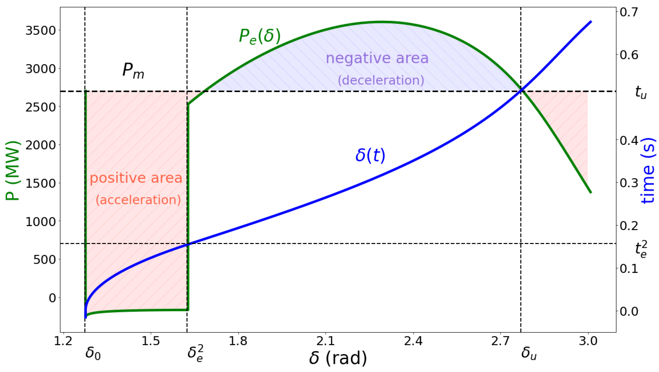
2.3. Approximations for Rapid Estimation of CCA
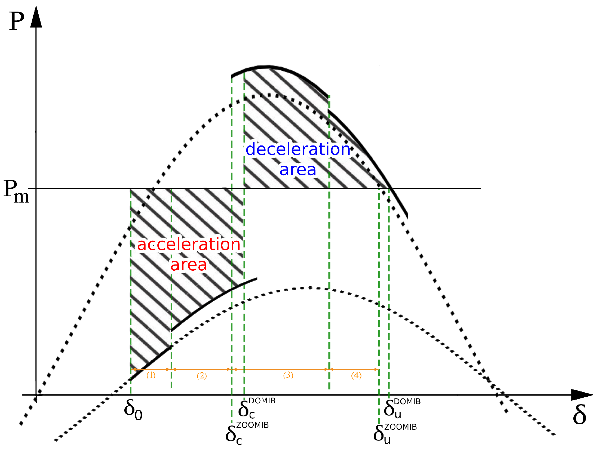
2.4. Definition and Conditions of OMIB Stability
2.5. The EEAC Functions
3. Critical Machines Identification and Critical Cluster Formation
3.1. Critical Machines Identification
3.1.1. Acceleration Criterion
3.1.2. Composite Criterion
3.1.3. Trajectory Criterion
3.2. Critical Cluster Formation
3.3. CMI and CCF Functions
4. Integration
5. Combining Algorithms for a Full-Resolution Scheme
6. Simulation Studies and Discussions
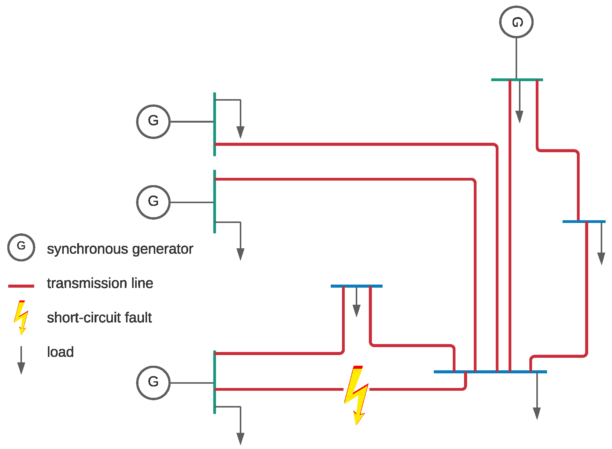
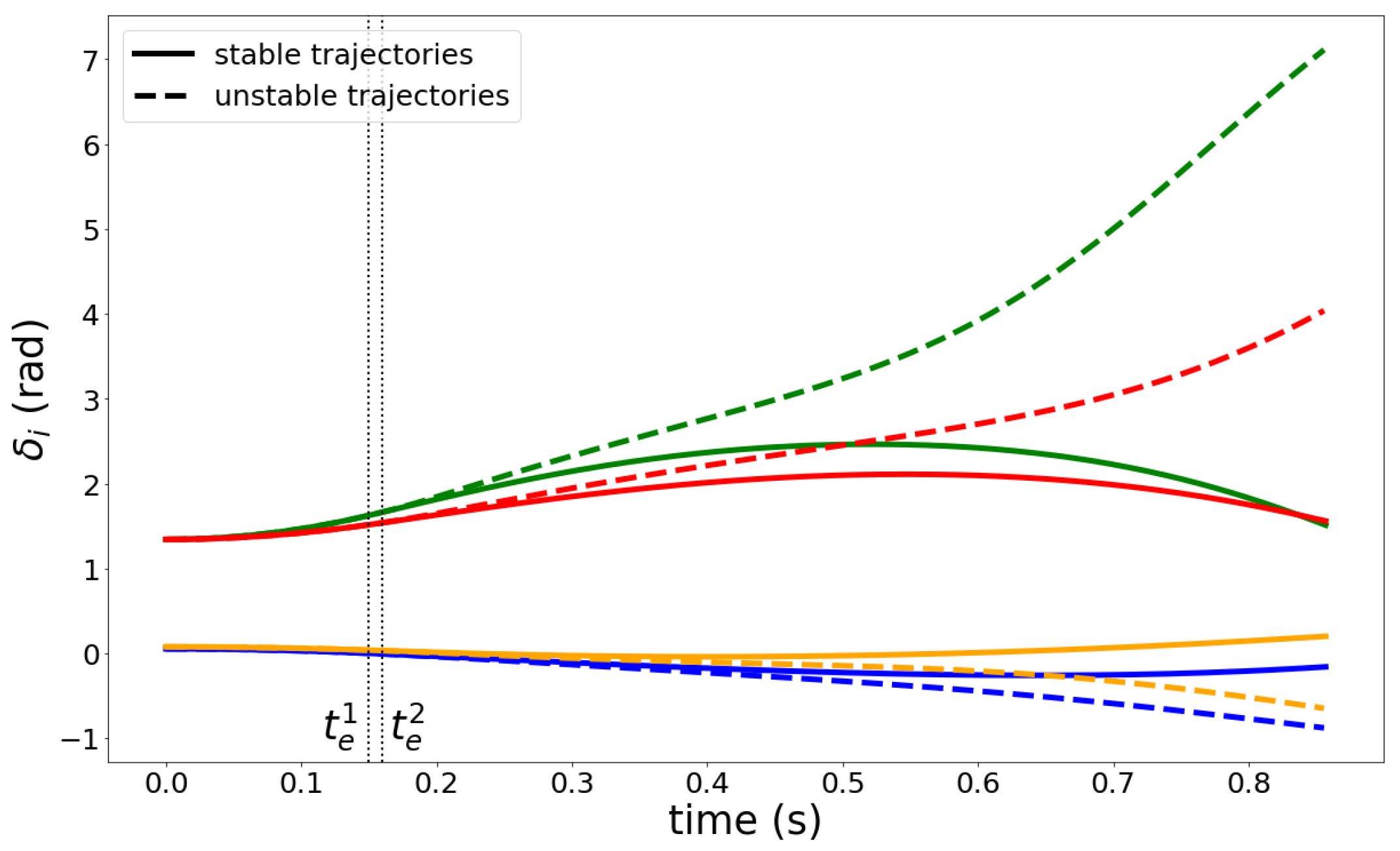
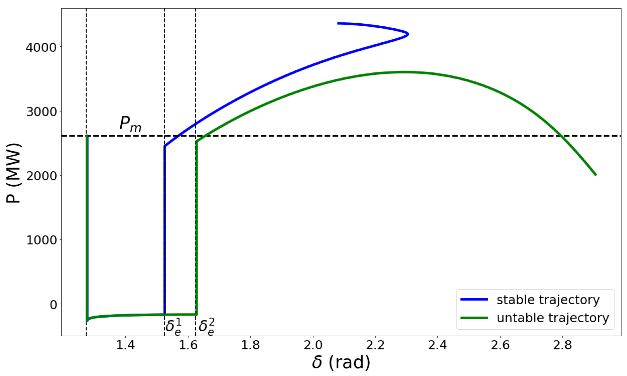
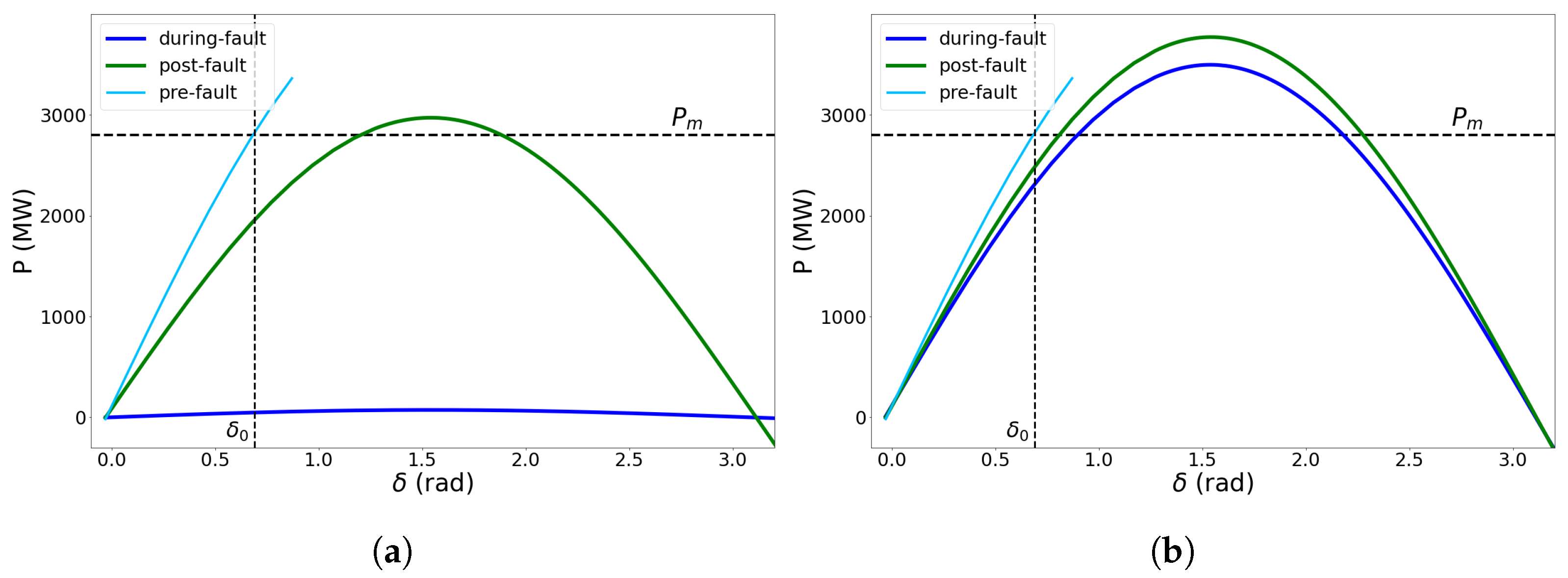
6.1. Four-Machine System
6.2. French Network
7. Conclusions
Author Contributions
Funding
Institutional Review Board Statement
Informed Consent Statement
Conflicts of Interest
Abbreviations
| TSO | Transmission System Operator |
| TSA | Transient Stability Analysis |
| EAC | Equal Area Criterion |
| EEAC | Extended Equal Area Criterion |
| OMIB | One-Machine Infinite Bus |
| SMIB | Single Machine connected to an Infinite Bus |
| SIME | Single-Machine Equivalent |
| CCT | Critical Clearing Time |
| CCA | Critical Clearing Angle |
| CMI | Critical Machines Identification |
| CCF | Critical Cluster Formation |
| CC | Critical Cluster of generators |
| NC | Non-critical Cluster of generators |
| COA | Center of Angle |
| PCOA | Partial Centre of Angle |
| ZOOMIB | Zero Offset OMIB |
| COOMIB | Constant Offset OMIB |
| DOMIB | Dynamic OMIB |
Appendix A. OMIB Electrical Power with the Classical Model
Appendix A.1. Considering Zero Rotor Angle Offsets with Respect to PCOA
Appendix A.2. Considering Constant Rotor Angle Offsets with Respect to PCOA
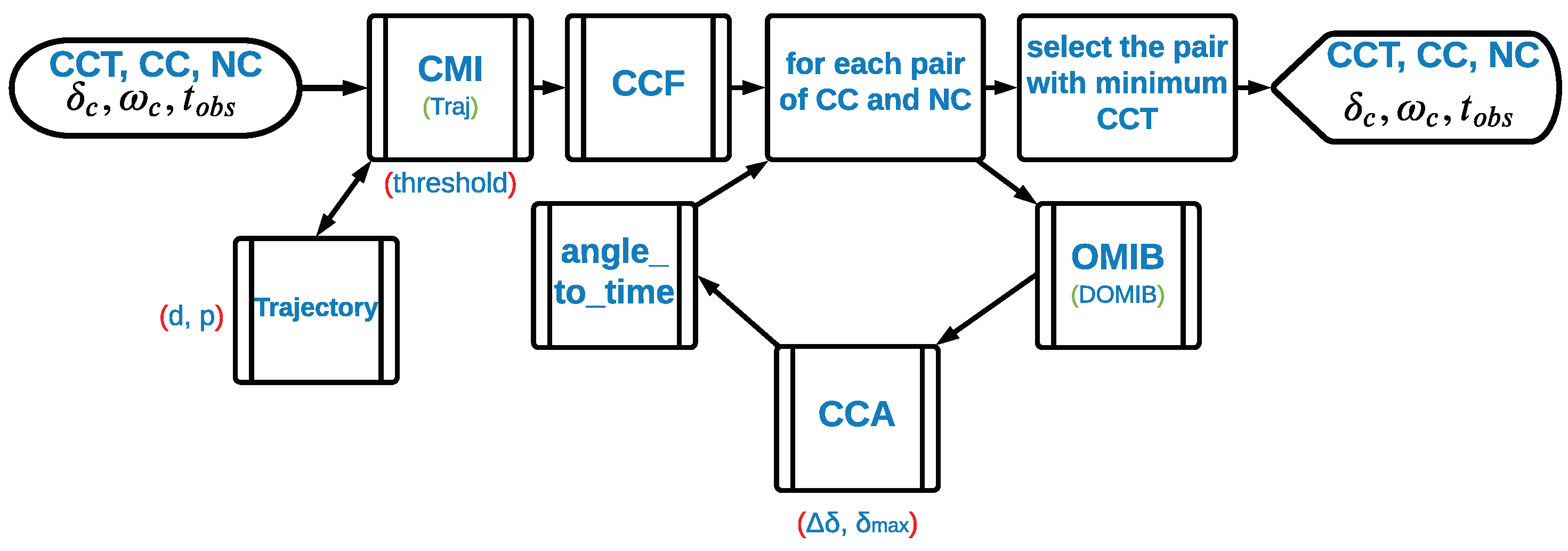
Appendix B. Pseudocodes
| Algorithm A1 Forming the OMIB equivalent of a multi-machine power system |
OMIB (, , , , , ) Input
Output
|
- : the intervals are continuous, the end of an interval corresponds to the beginning of the next one
- : the interval angles increase monotonically
- : the post-fault intervals include the maximum angle
- : the during-fault intervals include the initial angle
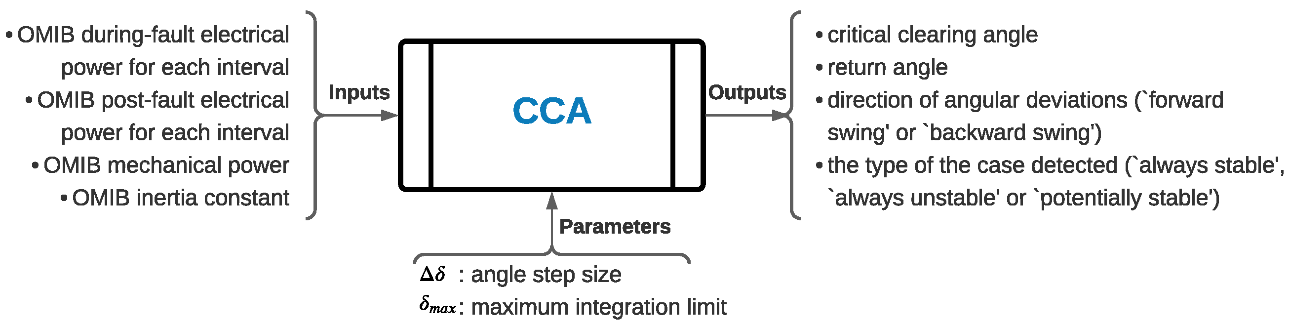
| Algorithm A2 Calculation of critical clearing angle of an OMIB model |
CCA (, ) Input
Output
Parameter
|
| Algorithm A3 Finding the area between and for desired and |
compute-area (, , ) Input
Output
|
| Algorithm A4 Finding electrical and mechanical powers at any desired angle |
compute-power (, ) Input
Output
|
| Algorithm A5 Returning the negated values of power vector elements |
negation () Input
Output
|
| Algorithm A6 Critical machines identification |
CMI (, , , , , , f, , ) Input
Output
Parameter
|
| Algorithm A7 Critical clusters formation |
CCF (, ) Input
Output
|
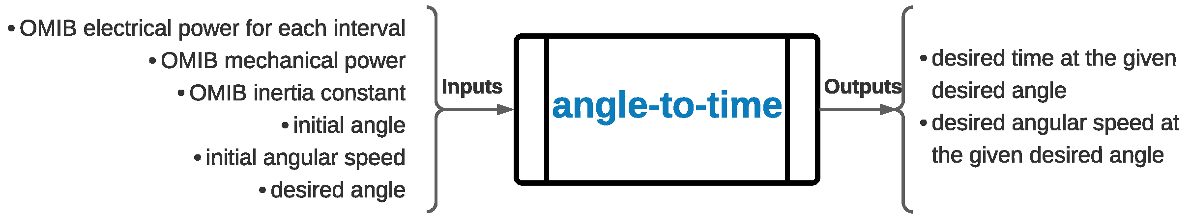
| Algorithm A8 Finding the time and angular speed associated to a desired angle for the OMIB model using the global Taylor series |
angle-to-time (, M, , , ) Input
Output
|
| Algorithm A9 Global Taylor series to find the OMIB time and angular speed associated with a desired angle, starting from an initial angle, time and angular speed |
GTS (, M, , , , i) Input
Output
Parameter
|
| Algorithm A10 Finding synchronous generators’ angle trajectory in time using an individual Taylor series |
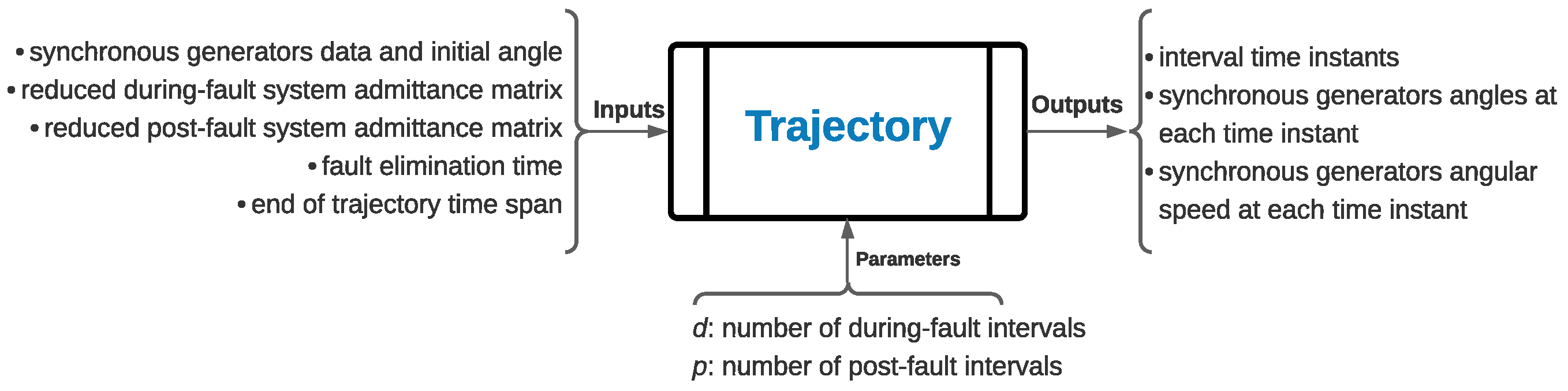
Trajectory (, , , , ) Input
Output
Parameter
|
| Algorithm A11 Individual Taylor series to find generators’ angle and angular speed at a desired time, starting from an initial angle and angular speed |
ITS (, , ,i) Input
Output
Parameter
|
| Algorithm A12 Basic scheme for EEAC |
basic-eeac (, , , , , , , f) Input
Output
Parameter
|
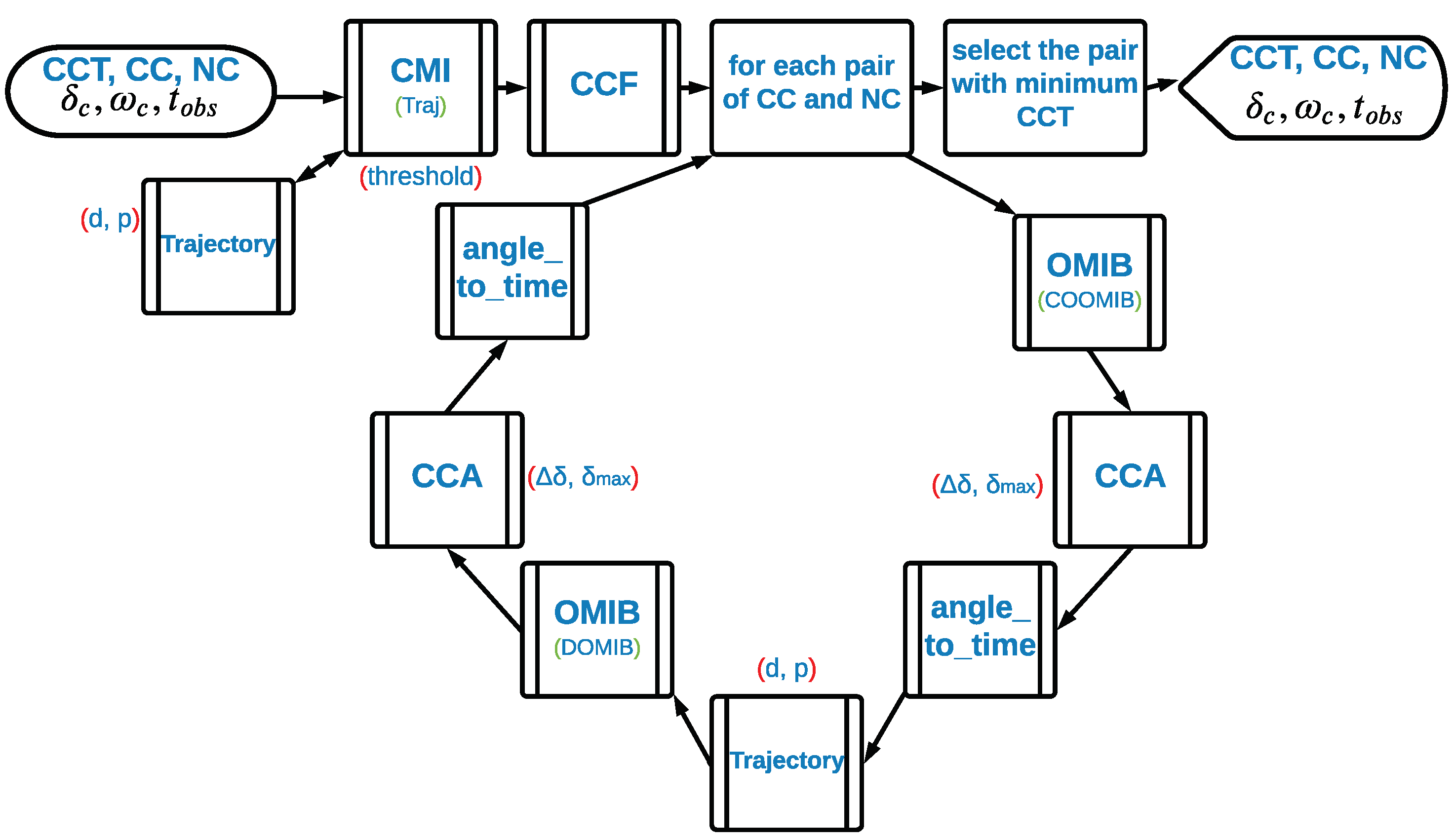
| Algorithm A13 Third refinement scheme for EEAC |
refinement-3 () Input
Output
Parameter
|
Appendix C. Taylor Series Expansion
Appendix C.1. Taylor Series for OMIB Equivalent
Appendix C.2. Taylor Series for an Individual Generator
References
- Pavella, M.; Ernst, D.; Ruiz-Vega, D. Transient Stability of Power Systems: A Unified Approach to Assessment and Control, 1st ed.; Springer Science & Business Media: New York, NY, USA, 2012. [Google Scholar]
- Dahl, O.G.C. Electric Circuits; Theory and Applications, 1st ed.; McGraw-Hill: New York, NY, USA, 1938. [Google Scholar]
- Skilling, H.H.; Yamakawa, M.H. A graphical solution of transient stability. Electrical Eng. 1940, 59, 462–465. [Google Scholar] [CrossRef]
- Kimbark, E.W. Power System Stability, 1st ed.; John Wiley & Sons: New York, NY, USA, 1948. [Google Scholar]
- Xue, Y.; Rousseaux, P.; Gao, Z.; Belhomme, R.; Euxible, E.; Heilbronn, B. A new decomposition method and direct criterion for trasient stability assessment of large-scale electric power systems. In Proceedings of the IMACS-IFAC Symposium on Modelling and Simulation for Control of Lumped and Distributed Parameter Systems, Lille, France, 3–6 June 1986. [Google Scholar]
- Xue, Y.; Van Cutsem, T.; Pavella, M. A simple direct method for fast transient stability assessment of large power systems. IEEE Trans. Power Syst. 1988, 3, 400–412. [Google Scholar] [CrossRef]
- Xue, Y.; Van Custem, T.; Pavella, M. Extended equal area criterion justifications, generalizations, applications. IEEE Trans. Power Syst. 1989, 4, 44–52. [Google Scholar] [CrossRef]
- Xue, Y.; Pavella, M. Extended equal-area criterion: An analytical ultra-fast method for transient stability assessment and preventive control of power systems. Int. J. Electrical Power Energy Syst. 1989, 11, 131–149. [Google Scholar] [CrossRef]
- Xue, Y.; Wehenkel, L.; Belhomme, R.; Rousseaux, P.; Pavella, M.; Euxibie, E.; Heilbronn, B.; Lesigne, J.-F. Extended equal area criterion revisited (EHV power systems). IEEE Trans. Power Syst. 1992, 7, 1127–1130. [Google Scholar] [CrossRef]
- Xue, Y.; Rousseaux, P.; Gao, Z.; Belhomme, R.; Euxible, E.; Heilbronn, B. Dynamic extended equal-area criterion. Part I: Basic formulation. Part II: Recent extensions. In Proceedings of the Athens Power Tech, Athens, Greece, 5–8 September 1993; pp. 889–900. [Google Scholar]
- Xue, Y.; Pavella, M. Extended equal area criterion justifications, generalizations, applications. IEE Proc. C 1993, 140, 481–489. [Google Scholar]
- Xue, Y.; Yu, Y.; Li, J.; Gao, A.; Ding, C.; Xue, F.; Wang, L.; Morison, G.K.; Kundur, P. A New Tool for Dynamic Security Assessment of Power Systems. In Proceedings of the IFAC/CIGRE Symposium on Control of Power Systems and Power Plants, Beijing, China, 12–15 August 1989; pp. 389–393. [Google Scholar] [CrossRef]
- Zhang, Y. Hybrid Extended EqualArea Criterion: A General Method for Transient Stability Assessment of Multimachine Power Systems. Ph.D. Thesis, University of Liége, Liége, Belgium, February 1995. [Google Scholar]
- Zhang, Y.; Wehenkel, L.; Rousseaux, P.; Pavella, M. SIME: A Hybrid Approach to Fast Transient Stability Assessment and Contingency Selection. J. EPES 1997, 119, 195–208. [Google Scholar] [CrossRef]
- Zhang, Y.; Wehenkel, L.; Pavella, M. SIME: Method for RealTime Transient Stability Emergency Control. In Proceedings of the CPSPP’97, IFAC/CIGRE Symp on Control of Power Systems and Power Plants, Beijing, China, 18–21 August 1997; pp. 673–678. [Google Scholar]
- Zhang, Y.; Wehenkel, L.; Pavella, M. SIME: A Comprehensive Approach to Fast Transient Stability Assessment. Trans. IEE Jpn. 1998, 118B, 127–133. [Google Scholar] [CrossRef] [Green Version]
- Ernst, D.; Bettiol, A.L.; RuizVega, D.; Wehenkel, L.; Pavella, M. Compensation Schemes for Transient Stability Assessment and Control. In Proceedings of the LESCOPE’98, Halifax, NS, Canada, 7–9 June 1998; pp. 225–230. [Google Scholar]
- Ernst, D.; Bettiol, A.L.; Zhang, Y.; Wehenkel, L.; Pavella, M. RealTime Transient Stability Emergency Control of the South-Southeast Brazilian System. In Proceedings of the SEPOPE’98, Curitiba, Brazil; 1998; pp. 1–9. Available online: https://www.researchgate.net/publication/224007124_Real-Time_Transient_Stability_Emergency_Control_of_the_South-Southeast_Brazilian_System (accessed on 30 September 2021).
- Ernst, D.; RuizVega, D.; Pavella, M. Preventive and Emergency Transient Stability Control. In Proceedings of the SEPOPE’2000, Curitiba, Brazil, 21–26 May 2000; pp. 1–10. Available online: https://www.researchgate.net/publication/229003465_Preventive_and_emergency_transient_stability_control (accessed on 30 September 2021).
- Ernst, D.; Ruiz-Vega, D.; Pavella, M.; Hirsch, P.; Sobajic, D. SIME: A Unified Approach to Transient Stability Contingency Filtering, Ranking and Assessment. IEEE Trans. Power Syst. 2001, 16, 435–443. [Google Scholar] [CrossRef]
- McNabb, P.; Bialek, J. A priori transient stability indicator of islanded power systems using extended equal area criterion. In Proceedings of the IEEE Power and Energy Society General Meeting, San Diego, CA, USA, 22–26 July 2012. [Google Scholar]
- Chen, C.; Tang, A.; Huang, Y.; Zheng, X.; Xu, Q. The Research of DPFC Considering EEAC. In Proceedings of the International Conference on Industrial Informatics-Computing Technology, Intelligent Technology, Industrial Information Integration, Wuhan, China, 2–3 December 2017; pp. 246–249. [Google Scholar] [CrossRef]
- Chenlu, W.; Xiaohua, Z.; Yuan, Z.; Chen, L.; Dezhuang, M. Impact identification of DFIG model on transient security analysis in power system. Energy Rep. 2020, 6, 307–311. [Google Scholar] [CrossRef]
- Li, Y.; Huang, S.; Li, H.; Zhang, J. Application of phase sequence exchange in emergency control of a multi-machine system. Int. J. Electr. Power Energy Syst. 2020, 121, 106136. [Google Scholar] [CrossRef]
- Li, F.; Wang, Q.; Tang, Y.; Xu, Y. An integrated method for critical clearing time prediction based on a model-driven and ensemble cost-sensitive data-driven scheme. Int. J. Electr. Power Energy Syst. 2021, 125, 106513. [Google Scholar] [CrossRef]
- Xue, Y.; Zhang, Y. Practical and Flexible Incorporation of AVR into Extended Equal Area Criterion. IFAC Proc. Vol. 1993, 26, 753–759. [Google Scholar] [CrossRef]
- Xue, Y.; Zhang, Y. Direct transient stability assessment with two-axis generator model. IFAC Proc. Vol. 1990, 23, 7–12. Available online: https://www.sciencedirect.com/science/article/pii/S1474667017513907 (accessed on 30 September 2021). [CrossRef]
- Xue, Y.; Sun, K. Generalized Equal Area Criterion for Transient Stability Analysis. In Proceedings of the 4th IEEE Conference on Energy Internet and Energy System Integration, Wuhun, China, 30 October–1 November 2020; pp. 2363–2368. [Google Scholar]
- Tao, Q.; Xue, Y.; Li, C. Transient Stability Analysis of AC/DC System Considering Electromagnetic Transient Model. In Proceedings of the IEEE Innovative Smart Grid Technologies, Chengdu, China, 21–24 May 2019; pp. 313–317. [Google Scholar]
- Pavella, M.; Murthy, P.G. Transient Stability of Power Systems, Theory and Practice, 1st ed.; John Wiley & Sons: Chichester, UK, 1993. [Google Scholar]
- Tavora, C.J.; Smith, O.J.M. Characterization of equilibrium and stability in power systems. IEEE Trans. Power App. Syst. 1972, 3, 1127–1130. [Google Scholar] [CrossRef]


| Assumptions and Approximations | True OMIB | ZOOMIB | COOMIB | DOMIB |
|---|---|---|---|---|
| Separation of generators to CC and NC | ✓ | ✓ | ✓ | ✓ |
| OMIB and have only one value for each | × | ✓ | ✓ | ✓ |
| Classical model for synchronous generators | × | ✓ | ✓ | ✓ |
| Constant offsets between generator angles and their receptive PCOA | × | ✓ | ✓ | (a) |
| Zero offsets between generator angles and their receptive PCOA | × | ✓ | × | × |
| Model | CCA (rad) | CCT (ms) |
|---|---|---|
| ZOOMIB | 1.084 | 199.58 |
| COOMIB | 1.085 | 199.96 |
| DOMIB | 1.038 | 189.15 |
| Time-domain with classical model | 1.036 | 187 |
| Time-domain with detailed model | 0.937 | 160 |
| Time-Domain | Basic Scheme ZOOMIB a | Basic Scheme COOMIB b | |||
|---|---|---|---|---|---|
| Scenario | CCT (ms) | CCT (ms) | Error (%) | CCT (ms) | Error (%) |
| 1 | 231 | 323.71 | −40.13 | 324.46 | −40.46 |
| 2 | 159 | 238.16 | 49.79 | 242.21 | −52.33 |
| 3 | 173 | 151.72 | −12.30 | 155.49 | 10.12 |
| 4 | 277 | 240.49 | −13.18 | 263.37 | 4.92 |
| 5 | 106 | 122.71 | 15.76 | 124.27 | −17.24 |
| 6 | 258 | unstable c | — | unstable | — |
| 7 | 227 | 159.41 | −29.78 | 167.35 | 26.28 |
| 8 | 225 | 203.00 | −9.78 | 210.20 | 6.58 |
| 9 | 195 | 216.84 | 11.20 | 221.99 | −13.84 |
| 10 | 205 | 234.20 | 14.24 | 239.63 | −16.89 |
| 11 | 184 | 202.48 | 10.04 | 207.15 | −12.58 |
| 12 | 198 | 227.26 | 14.78 | 232.42 | −17.38 |
| 13 | 182 | 201.31 | 10.61 | 205.15 | −12.72 |
| 14 | 189 | 217.11 | 14.87 | 221.58 | −17.24 |
| 15 | 267 | 286.32 | 7.24 | 295.36 | −10.62 |
| 16 | 259 | 279.33 | 7.85 | 288.07 | −11.22 |
| 17 | 258 | 280.43 | 8.69 | 288.68 | −11.89 |
| 18 | 159 | 18.74 | −88.21 | 57.62 | 63.76 |
| 19 | 135 | 136.73 | 1.28 | 132.62 | 1.76 |
| 20 | 119 | 233.84 | 96.50 | 222.42 | −86.90 |
| 21 | 98 | 217.54 | 121.98 | 202.96 | −107.11 |
| 22 | 95 | 77.97 | −17.93 | 68.14 | 28.27 |
| 23 | 104 | 81.34 | −21.78 | 73.70 | 29.14 |
| 24 | 120 | 111.19 | −7.34 | 104.83 | 12.64 |
| 25 | 124 | 116.86 | −5.76 | 110.56 | 10.84 |
| 26 | 105 | 79.86 | −23.95 | 72.64 | 30.82 |
| 27 | 129 | 125.42 | −2.78 | 122.28 | 5.21 |
| 28 | 129 | 126.42 | −2.00 | 122.28 | 5.21 |
| 29 | 129 | 124.75 | −3.30 | 120.43 | 6.65 |
| 30 | 122 | 112.53 | −7.76 | 106.80 | 12.46 |
| 31 | 126 | 115.95 | −7.98 | 110.49 | 12.31 |
| 32 | 140 | 146.38 | 4.56 | 143.14 | −2.25 |
| 33 | 142 | 148.51 | 4.58 | 145.43 | −2.42 |
| minimum d | 95 | 18.74 | 1.28 | 57.62 | 1.76 |
| maximum d | 277 | 323.71 | 121.98 | 324.46 | 107.11 |
| mean d | 168.76 | 173.70 | 21.50 | 175.12 | 21.88 |
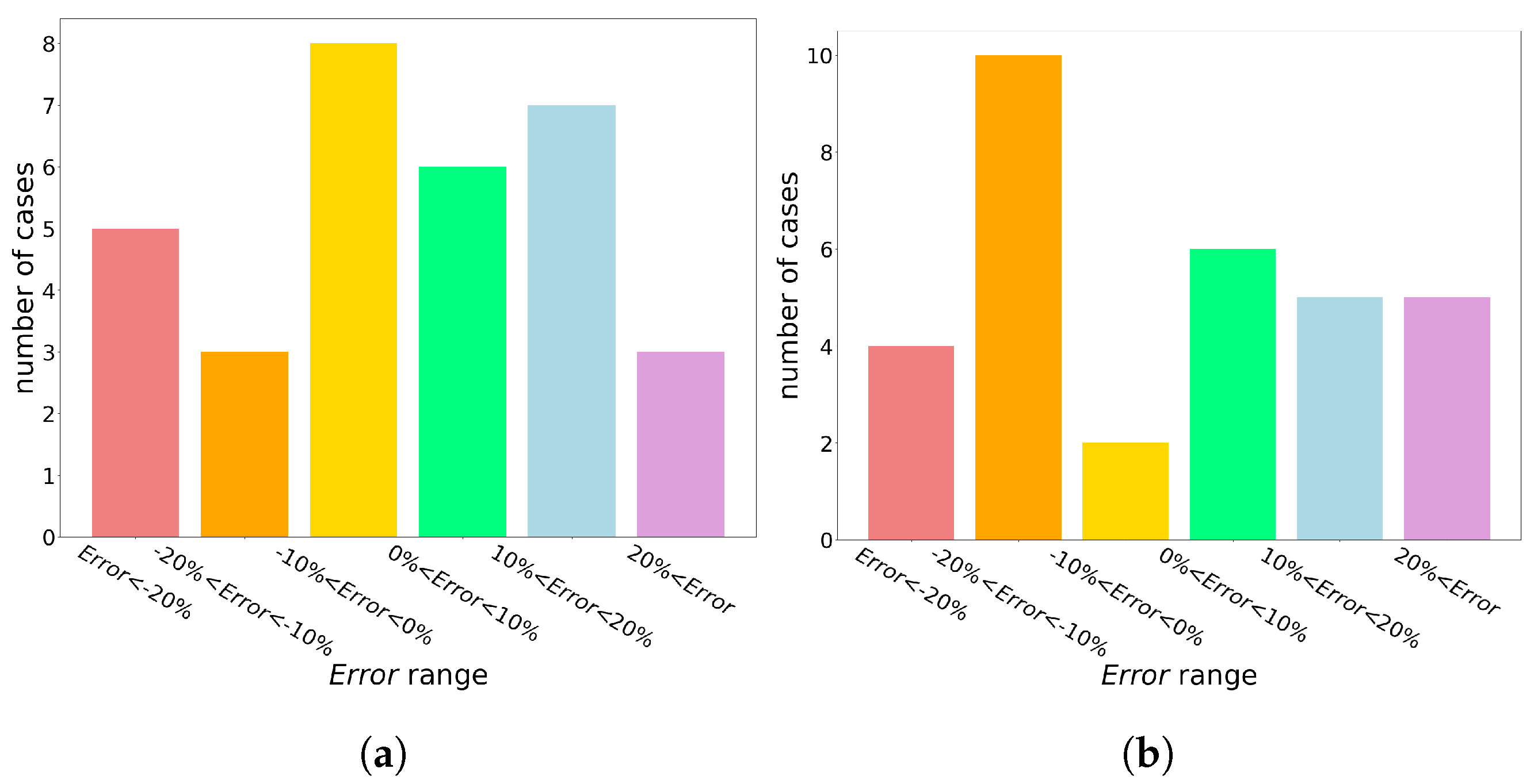
| Time-Domain | First Refinement Scheme a | Second Refinement Scheme a | Third Refinement Scheme a | ||||
|---|---|---|---|---|---|---|---|
| Scenario | CCT (ms) | CCT (ms) | Error (%) | CCT (ms) | Error (%) | CCT (ms) | Error (%) |
| 1 | 231 | unstable b | — | 586.39 | −153.85 | stable c | — |
| 2 | 159 | 235.91 | −48.37 | 235.91 | −48.37 | 235.86 | −48.34 |
| 3 | 173 | 132.53 | 23.39 | 132.53 | 23.39 | 133.18 | 23.02 |
| 4 | 277 | 262.31 | 5.30 | 262.31 | 5.30 | 265.41 | 4.18 |
| 5 | 106 | 119.10 | −12.36 | 119.10 | −12.36 | 119.10 | −12.36 |
| 6 | 258 | unstable | — | unstable | — | unstable | — |
| 7 | 227 | 161.43 | 28.89 | 150.50 | 33.70 | unstable | — |
| 8 | 225 | 208.27 | 7.43 | 197.83 | 12.08 | unstable | — |
| 9 | 195 | 232.52 | −19.24 | 232.52 | −19.24 | unstable | — |
| 10 | 205 | 255.70 | −24.73 | 255.70 | −24.73 | 245.51 | −19.76 |
| 11 | 184 | 215.32 | −17.02 | 215.32 | −17.02 | 201.38 | −9.44 |
| 12 | 198 | 249.73 | −26.12 | 249.73 | −26.12 | 241.21 | −21.82 |
| 13 | 182 | 212.02 | −16.49 | 212.02 | −16.49 | 194.26 | −6.73 |
| 14 | 189 | 236.59 | −25.18 | 236.59 | −25.18 | 229.82 | −21.60 |
| 15 | 267 | 306.82 | −14.91 | 306.82 | −14.91 | unstable | — |
| 16 | 259 | 299.81 | −15.76 | 299.81 | −15.76 | 294.38 | −13.66 |
| 17 | 258 | failed | — | 354.87 | −37.54 | 294.26 | -14.05 |
| 18 | 159 | 48.41 | 69.55 | stable | — | stable | — |
| 19 | 135 | 129.99 | 3.71 | 129.99 | 3.71 | unstable | — |
| 20 | 119 | 209.06 | −75.68 | 209.06 | −75.68 | 209.73 | −76.25 |
| 21 | 98 | 187.45 | −91.28 | 187.45 | −91.28 | 188.22 | −92.06 |
| 22 | 95 | 52.14 | 45.12 | stable | — | stable | — |
| 23 | 104 | 55.27 | 46.85 | stable | — | stable | — |
| 24 | 120 | 100.46 | 16.29 | 100.46 | 16.29 | 94.12 | 21.57 |
| 25 | 124 | 105.90 | 14.60 | 105.90 | 14.60 | 99.90 | 19.43 |
| 26 | 105 | 53.55 | 49.00 | stable | — | stable | — |
| 27 | 129 | 107.96 | 16.31 | 104.46 | 19.02 | unstable | — |
| 28 | 129 | 107.96 | 16.31 | 104.46 | 19.02 | unstable | — |
| 29 | 129 | 105.74 | 18.03 | 101.42 | 21.38 | unstable | — |
| 30 | 122 | 89.31 | 26.79 | 84.40 | 30.82 | unstable | — |
| 31 | 126 | 92.79 | 26.36 | 88.10 | 30.08 | unstable | — |
| 32 | 140 | 130.88 | 6.51 | 128.05 | 8.53 | 122.12 | 12.77 |
| 33 | 142 | 132.88 | 6.42 | 130.16 | 8.34 | 120.40 | 15.21 |
| minimum d | 95 | 48.41 | 3.71 | 84.40 | 3.71 | 94.12 | 4.18 |
| maximum d | 277 | 306.82 | 91.28 | 586.39 | 153.85 | 294.38 | 92.06 |
| mean d | 168.76 | 161.26 | 27.13 | 197.21 | 29.46 | 193.46 | 25.43 |
Publisher’s Note: MDPI stays neutral with regard to jurisdictional claims in published maps and institutional affiliations. |
© 2021 by the authors. Licensee MDPI, Basel, Switzerland. This article is an open access article distributed under the terms and conditions of the Creative Commons Attribution (CC BY) license (https://creativecommons.org/licenses/by/4.0/).
Share and Cite
Bahmanyar, A.; Ernst, D.; Vanaubel, Y.; Gemine, Q.; Pache, C.; Panciatici, P. Extended Equal Area Criterion Revisited: A Direct Method for Fast Transient Stability Analysis. Energies 2021, 14, 7259. https://doi.org/10.3390/en14217259
Bahmanyar A, Ernst D, Vanaubel Y, Gemine Q, Pache C, Panciatici P. Extended Equal Area Criterion Revisited: A Direct Method for Fast Transient Stability Analysis. Energies. 2021; 14(21):7259. https://doi.org/10.3390/en14217259
Chicago/Turabian StyleBahmanyar, Alireza, Damien Ernst, Yves Vanaubel, Quentin Gemine, Camille Pache, and Patrick Panciatici. 2021. "Extended Equal Area Criterion Revisited: A Direct Method for Fast Transient Stability Analysis" Energies 14, no. 21: 7259. https://doi.org/10.3390/en14217259
APA StyleBahmanyar, A., Ernst, D., Vanaubel, Y., Gemine, Q., Pache, C., & Panciatici, P. (2021). Extended Equal Area Criterion Revisited: A Direct Method for Fast Transient Stability Analysis. Energies, 14(21), 7259. https://doi.org/10.3390/en14217259