Abstract
The global maximum power point tracking of a PV array under partial shading represents a global optimization problem. Conventional maximum power point tracking algorithms fail to track the global maximum power point, and global optimization algorithms do not provide global maximum power point in real-time mode due to a slow convergence process. This paper presents an intelligent reconfigurable photovoltaic system on the basis of a modified fuzzy neural net that includes a convolutional block, recurrent networks, and fuzzy units. We tune the modified fuzzy neural net based on modified multi-dimension particle swarm optimization. Based on the processing of the sensors’ signals and the photovoltaic array’s image, the tuned modified fuzzy neural net generates an electrical interconnection matrix of a photovoltaic total-cross-tied array, which reaches the global maximum power point under non-homogeneous insolation. Thus, the intelligent reconfigurable photovoltaic system represents an effective machine learning application in a photovoltaic system. We demonstrate the advantages of the created intelligent reconfigurable photovoltaic system by simulations. The simulation results reveal robustness against photovoltaic system uncertainties and better performance and control speed of the proposed intelligent reconfigurable photovoltaic system under non-homogeneous insolation as compared to a GA-based reconfiguration total-cross-tied photovoltaic system.
1. Introduction
The power generated by a photovoltaic (PV) array depends on temperature, insolation, and partial shading (PS) [1]. The generated PV array power significantly decreases due to PS, which is difficult to track and forecast. According to statistical studies, the power loss can vary from 10% to 70% due to PS [2]. The power–voltage (P–V) characteristic of a PV array under PS has several peaks. Thus, the global maximum power point (GMPP) tracking of a PV array under PS represents a global optimization problem. Conventional maximum power point tracking (MPPT) algorithms, such as Perturb and Observe, fail to track the GMPP [1].
There are many global optimization algorithms that can be implemented in an MPPT controller [1,3], but all of them have the following drawbacks: power oscillations in the steady state; the fact that the initialization process is a crucial issue affecting performance; slow convergence to a GMPP under fluctuation of the insolation; and the fact that during slow changing of the insolation, the alteration of the control signal needs to be small in order to track the GMPP properly. Because of these drawbacks, these algorithms do not provide GMPP of a PV system in real-time mode. In [4], we presented the intelligent PV system on the basis of the modified fuzzy neural net (MFNN), which shows impressive robustness, performance, and control speed in tracking the GMPP under PS. The MFNN represents an effective machine learning method [5]. Compared to existing fuzzy neural nets, including the adaptive network-based fuzzy inference system, the MFNN includes recurrent neural nets. We exploit the function approximation capabilities of a recurrent neural net to approximate a membership function.
One of the technical options to maximize the generated PV array power under PS is to change the electrical interconnection of a reconfigurable PV array [6,7,8,9]. There are many structures of a reconfigurable PV array, such as series-parallel, honey-comb, and total-cross-tied (TCT) arrays. [6,7]. The papers [8,9] reported that the TCT structure is the best to decrease losses under PS. The most-common reconfiguration approach is the insolation equalization method [7]. Within an optimization approach, the paper [10] presented a reconfiguration scheme to increase PV array power generation under PS based on a genetic algorithm. Therefore, the usage of the MFNN for maximum power point tracking of a reconfigurable TCT PV system is a promising alternative. This forms the motivation to maximize the generated PV array power by generating the PV array’s interconnection matrix and control signal on the basis of the MFNN. In this paper, we consider a non-linear GMPP tracking of a reconfigurable PV array under PS on the basis of the MFNN. The objective of this study is the creation of an intelligent reconfigurable PV system on the basis of the MFNN to maximize the generated PV array power under PS. Future research will be directed towards applying a software implementation of the developed and verified intelligent reconfigurable PV system in a programmable MPPT controller.
The remainder of this paper proceeds as follows: Section 2 presents an intelligent reconfigurable PV system on the basis of an MFNN that fully harvests solar energy. Section 2.1 describes the proposed TCT PV array reconfiguration algorithm based on particle swarm optimization (PSO), which homogeneously distributes a shadow among PV modules. Section 2.2 provides a description of the intelligent reconfigurable PV system on the basis of the MFNN, which tracks GMPP and optimal configuration of a TCT PV array. For the purpose of organizing intelligent computing as an optimum structure in this research, the MFNN includes one convolutional block and a recurrent neural net (RNN), fuzzy units, and RNNs. In order to automatically define the optimal architecture of an MFFN that demands global multi-dimensional optimization and definition of conditions of optimal MFFN architecture, we improved modified PSO [5] based on a quantum-behaved PSO algorithm with Laplace distribution (QPSO-LD) [11] and the proposed hierarchical encoder of the dimension component of particles. We tuned the MFNN based on a modified multidimension quantum-behaved PSO algorithm with Laplace distribution (MD QPSO-LD). Section 3 presents a comparative simulations study and analysis of the results of the intelligent reconfigurable PV system on the basis of the tuned MFNN when compared against a reconfigurable TCT PV system based on GA. Based on processing of the signals from basic sensors and the TCT PV array’s image, the proposed intelligent reconfigurable PV system on the basis of the tuned MFNN generates the PV array’s interconnection matrix and control signal, which provide the PV array’s GMMP under PS in real-time mode. Finally, in Section 4, we conclude the paper with a brief summary. The simulation results reveal robustness to PV system uncertainties and better performance and control speed of the proposed intelligent reconfigurable PV system under PS as compared to a reconfigurable TCT PV system based on GA.
2. Materials and Methods
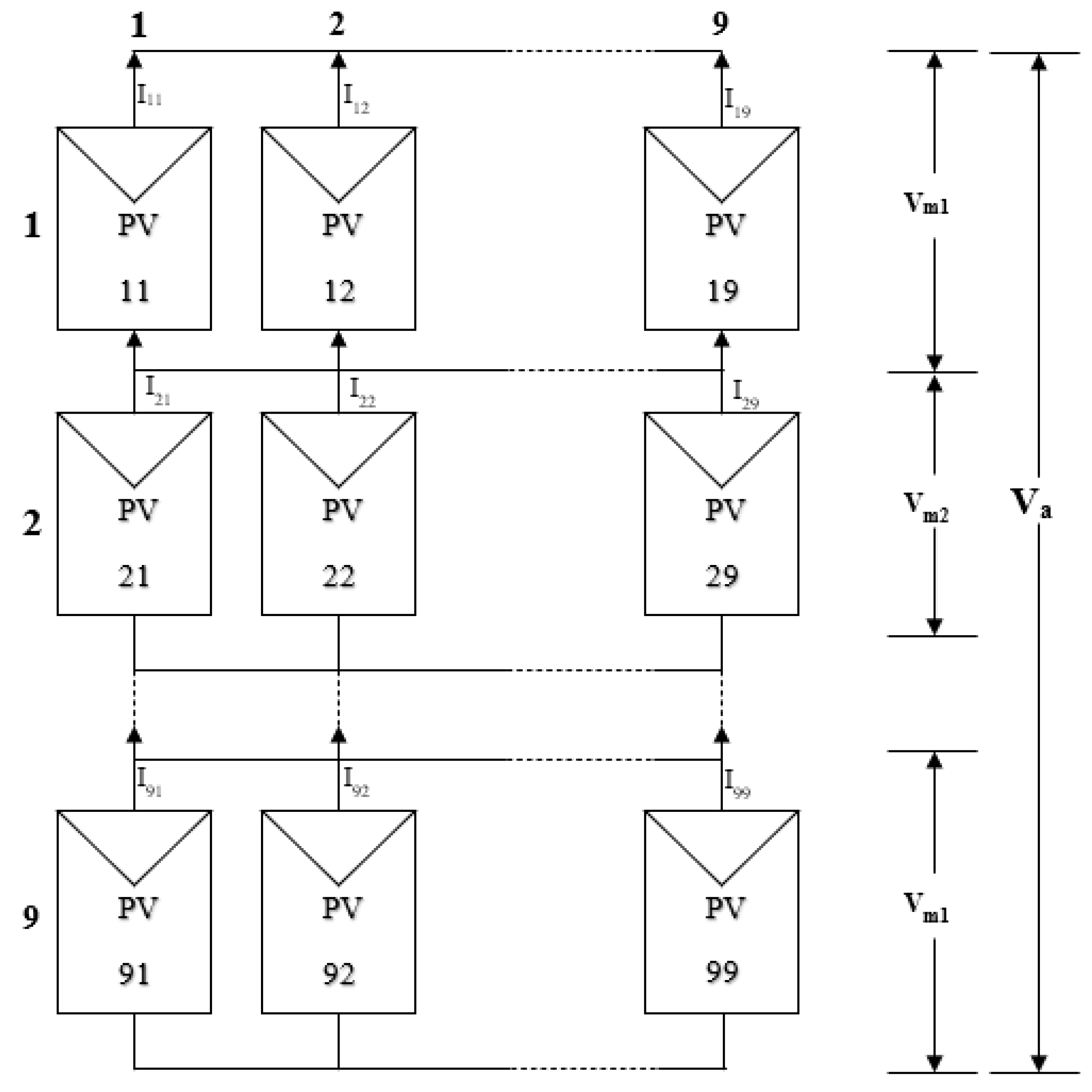
We designed and simulated using the author’s software “The intellectual controller of a non-linear technical system” [12], a TCT-configured 20 kW PV array that includes 81 PV modules. Table 1 presents the PV module’s specifications at standard test conditions (irradiance is ; temperature is 25 °C). The modules are tagged with “rc”, where “r” represents the row and “c” shows the column in which the module is connected,. Figure 1 illustrates the configuration of this PV array.

Table 1.
Specifications for YL245P-29b PV module at standard test conditions.
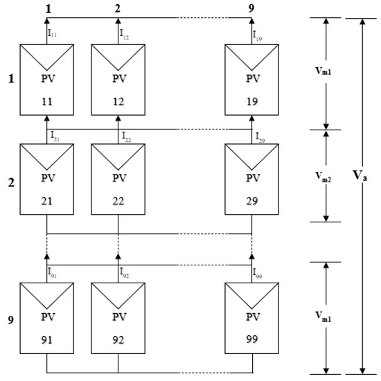
Figure 1.
Configuration of PV array.
We calculated the PV module’s current under an insolation G as
where is the PV module’s current.
We calculated the PV array’s voltage as
where is the voltage of the modules at the ith row.
We calculated the PV array node’s current by Kirchhoff’s current law as follows:
where is the current of the module at the ith row, the jth column.
2.1. The Proposed TCT PV Array’ Reconfiguration Algorithm Based on PSO
We coded the PV array’s interconnection matrix as the particle’s X positions . We defined the objective function as
where and are voltage across the PV array for current limit of rth row and the current limit, respectively; is weights; is the maximum possible value of current when bypassing is considered; and P is PV module’s output power when bypassing is not considered.
We expressed the proposed TCT PV array’s reconfiguration algorithm based on PSO as Algorithm 1:
| Algorithm 1. The TCT PV Array’ Reconfiguration Algorithm Based on PSO. |
| Step 0. We initialize the particle’s positions as the present PV array’s interconnection matrix. Step 1. For do initialize the particle’s positions xX,0c~U(1, 81), . Initialize the particle’s best-known position. If then Do: End If. If Then Do End If. End For. Step 2. While a convergence criterion is not met do: For do: For do: Pick random numbers: r1, r2 ~ U(0,1), update the particle’s velocity: . If then Do: else End If. If Then Do End If. End For. End For. |
2.2. The Intelligent Reconfigurable PV System on the Basis of the MFNN
We tuned the MFNN based on the experimental data:
where is resized image to 224 × 224 pixel of PV array; and are the array’s current and voltage, respectively;is the PV array’s power; and are power and voltage of the PV array at GMMP, respectively; is insolation; and is the PV array’s interconnection matrix at GMMP.
The temperature’s variation of each example from the data (5) does not exceed 0.1 °C per minute. Thus, the MFNN in this study mostly focuses on the partial shading because partial shading has more of an impact on power generation and has more complex shot-term dynamics as compared to temperature. The dataset (5) represents the samples of the 20 kW PV array’s signals under PS from the SCADA database. The Abakan solar plant includes this PV array. This database was collected at the site of Abakan (91.4° of longitude East, 53.7° of latitude North and 246 m of altitude) from 31 January 2018 to December 2018.
We obtained the dataset (5) based on numerical experiments from Section 2.1 (in order to fully harvest PV array energy by the homogeneous distribution of a shadow among PV modules) based on the proposed algorithm 1 “The TCT PV array’s reconfiguration algorithm based on PSO”. We validated all TCT PV array configuration schemes in Matlab/Simulink. We implemented the proposed algorithm 1 “The TCT PV array’s reconfiguration algorithm based on PSO” using the author’s software “The multi-agent adaptive fuzzy neuronet” [13].
In this research, the MFNN includes a convolutional block, a two-layer RNN, fuzzy units, and two two-layered RNNs. We coded the MFNN architecture’s parameters (a number of hidden neurons is, corresponded weights and biases, and a number of RNN’s delays—) into particles X. In this research, the dimension of particle X is .
2.2.1. The Creation of an Optimum MFNN’s Architecture Based on a Modified MD QPSO-LD
We defined a fitness function as
where H is number of evaluated samples and is the power of the intelligent reconfigurable PV system based on the MFNN with architecture X. We coded the dimension component of particle X as The number of all is 9261.
We describe the modified MD QPSO-LD for creating an optimum architecture of the MFNN (the termination criteria are is the number of particles) as Algorithm 2:
| Algorithm 2. The modified MD QPSO-LD. |
| Step 1.1. Fordo: Generate ,—current coded dimension of X position, . Initialize , —personal best coded dimension of position X. For do: Generate based on Nguyen–Widrow method; —jth component of the particle X position (represents the jth MFNN architecture’s parameters ) in coded dimension Initialize , —jth component of the global best swarm position in coded dimension d. End For. End For. Step 1.2. For do: For do: If then Do: If then else End If. Else End If. If then Do: , g(d) represents the index of the global best swarm particle in coded dimension If then ; —global best swarm’ coded dimension End If. End If. In other coded dimensions do updates , . End For. If OR then Stop. End If. Step 1.3. While OR is the Jacobian matrix, and is the learning rate. Step 1.4. Calculate , , If then ; ; ; Go to step 3 else ; go to step 4 end If. Step 1.5. For do: For do: Generate u and k as U(0,1); and G has Laplace distribution; is contraction–expansion coefficient; In other coded dimensions do updates . End For. Compute , End For. End For. |
The proposed modified MD QPSO-LD provides an inter-dimensional quantum-behaved search of swarm particles for both positional and dimensional optimum by the hierarchical encoded dimensional components, which decode into the real dimensions of particles. The proposed modified MD QPSO-LD automatically creates an optimum architecture of the MFFN, , and provides a global best swarm-coded dimension, .
2.2.2. The Generation of an Intelligent Reconfigurable PV System on the Basis of the MFNN
We created the intelligent reconfigurable PV system on the basis of the MFNN as follows:
Step 2.1. We create the convolutional block with output filter size 11 and then an RNN . The and are input and target, respectively. The RNN approximates the PV array’s interconnection matrix at GMMP.
Step 2.2. We define the fuzzy sets ( is “big reconfiguration of a PV array”, is “small reconfiguration of a PV array”) with membership functions based on the RNN’s output as follows:
Step 2.3. We create the MFNN, which includes the convolutional block, the RNN and the RNNs The MFNN architecture’s parameters (number of delays, corresponded weights, and biases of nodes in hidden layers) were coded into particles X.
We tune the MFNN by algorithm 2 “The modified MD QPSO-LD”. This provides the best solution X created by modified MD QPSO-LD, the tuned MFNN , which generates the PV array’s interconnection matrix at GMMP and the control signal .
We define the MFNN by if–then rules as:
2.2.3. The Simulation of an Intelligent Reconfigurable PV System on the Basis of the MFNN
We briefly describe the simulation of the intelligent reconfigurable PV system on the basis of the tuned MFNN as follows:
Step 3.1. The PV modules change their electrical interconnections accordingly with , which approximates the PV array’s interconnection matrix at GMMP. Aggregation antecedents of rules (8) map input data into their membership functions.
Step 3.2. Step 1 triggers the rule, which corresponds to the PV array mode. The RNN generates the control signal .
Based on processing of the input signals , the proposed intelligent reconfigurable PV system on the basis of the tuned MFNN generates the PV array’s interconnection matrix and control signal, which provide the PV array’s GMMP.
3. Results and Discussion
We fulfilled the intelligent reconfigurable PV system on the basis of the tuned MFNN using the author’s software [12,13,14]. We tuned the MFNN based on algorithm 2 “The modified MD QPSO-LD” and the training set of data (4) . In order to achieve statistical results, we fulfilled 100 modified PSO and modified MD QPSO-LD runs with parameters: (the number of particles) and (the maximum number of iterations is 450). Figure 2 shows that the modified MD QPSO-LD clearly has a higher convergence speed than the modified PSO on the basis of the MFNN over the training set of data (5).
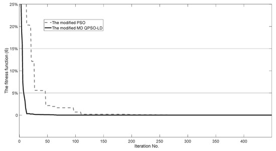
Figure 2.
The mean convergence curves.
The usage of the Laplace distribution to generate the swarm particles’ positions creates an effective MFNN architecture at initial iterations, and the quantum-behaved PSO algorithm speeds up the convergence of the modified MD QPSO-LD as compared to the modified PSO.
The modified MD QPSO-LD creates the optimum architecture of the MFFN with . This MFNN includes a convolutional block, the two-layered RNN with five hidden neurons (number of delays is two), and the two two-layered RNNs with five hidden neurons (number of delays is two).
In this comparative research, the performance of the intelligent reconfigurable PV system on the basis of the tuned MFNN is compared with a reconfigurable TCT PV system based on GA. We implemented the reconfigurable TCT PV system based on GA as described in [10].
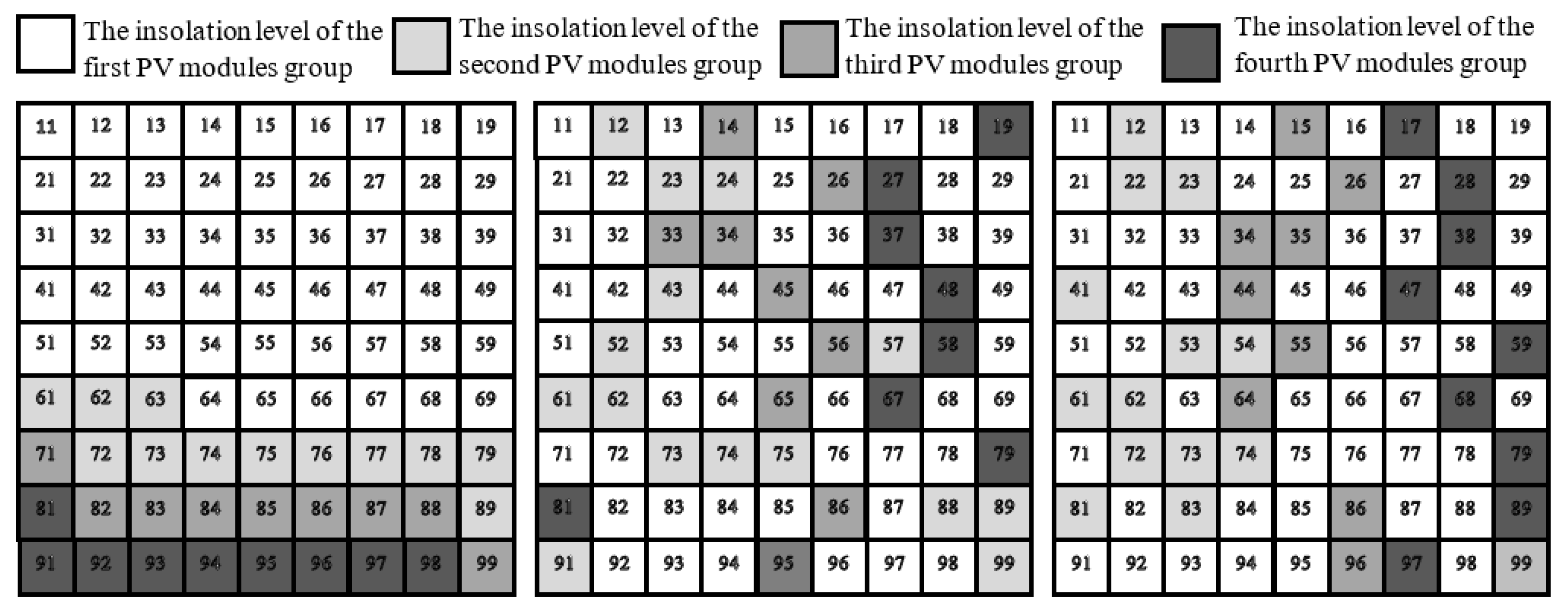
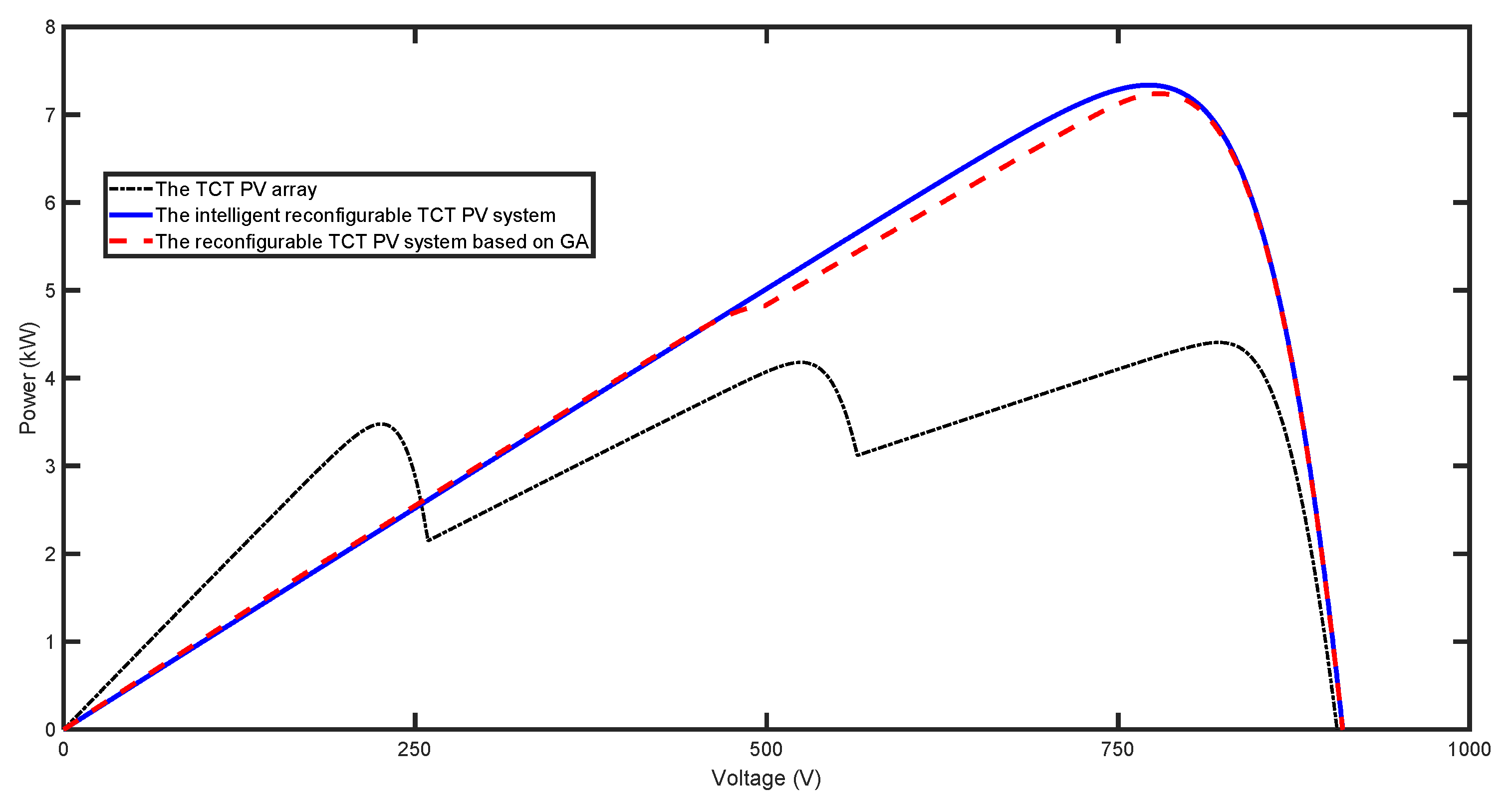
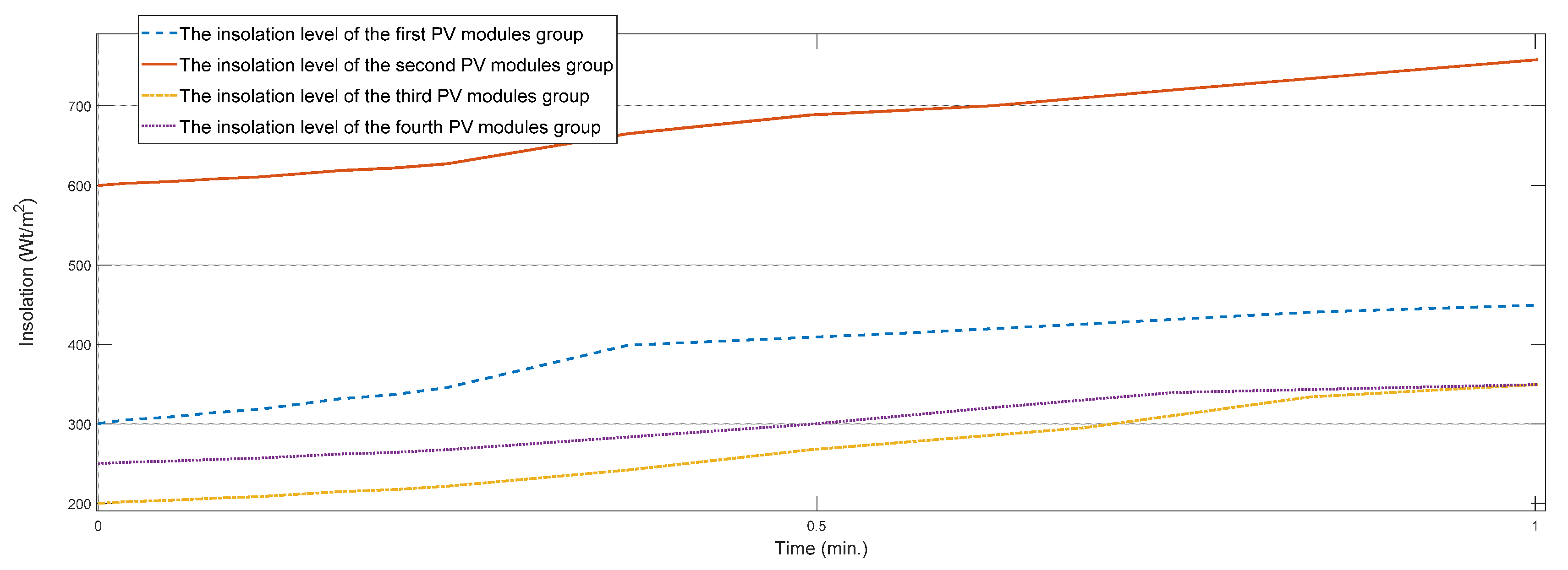
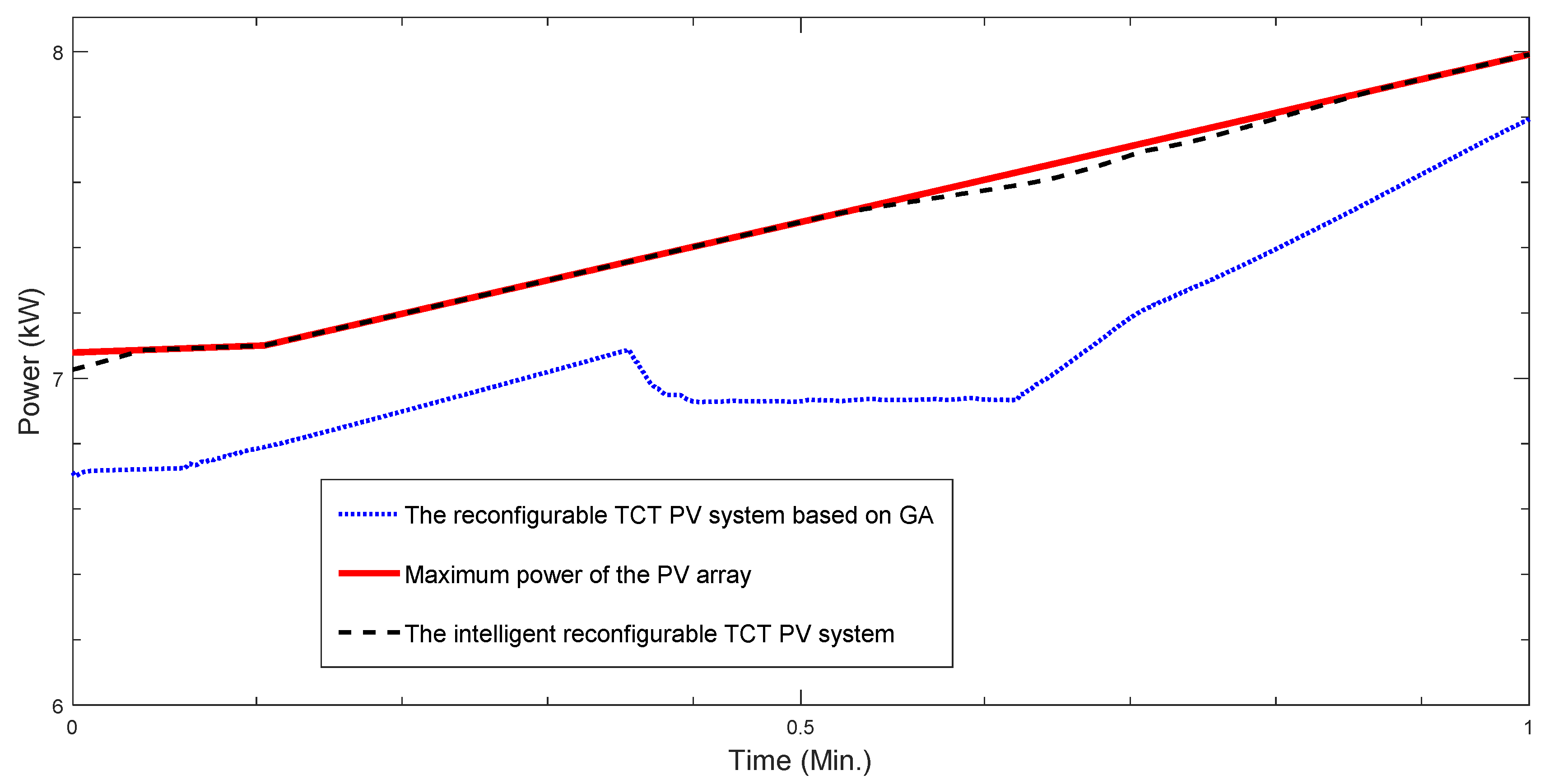
Figure 3 shows an example ( of a PV array under PS that has implemented the most common cases of self-shading (especially during the winter in the morning and evening). Figure 3 displays a TCT PV array’s scheme and two configuration PV array schemes, which were generated by the intelligent reconfigurable PV system and the reconfigurable TCT PV system based on GA, respectively. We generated Inj the insolation level of the jth PV modules group based on . Figure 4 presents the P–V curves of these reconfiguration schemes in the first second (In = (600 W/m2, 300 W/m2, 250 W/m2,200 W/m2)), . Figure 5 shows the insolation levels’ dynamics of the four PV module groups for this example,. Each module remains in the same PV module group despite the insolation dynamics of these PV module groups during the example’s time . Figure 6 indicates that the proposed intelligent reconfigurable PV system is more robust and provides more energy than does the reconfigurable TCT PV system based on GA. Figure 6 shows that the reconfigurable TCT PV system based on GA does not provide GMPP in such a case, because it activates the initialization procedure for genes under changing PS and does not complete the optimization process in real-time mode.
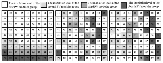
Figure 3.
The configuration scheme provided by the TCT PV array, the intelligent reconfigurable PV system, and the reconfigurable TCT PV system based on GA.
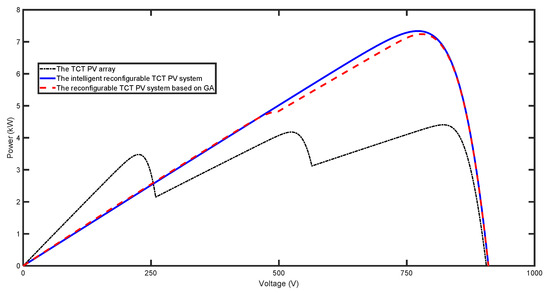
Figure 4.
The P–V curves of PV array reconfiguration schemes.
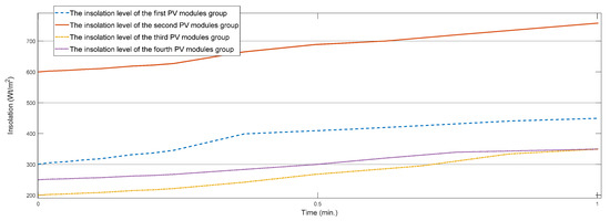
Figure 5.
The dynamics of PV array insolation levels.
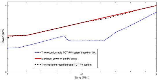
Figure 6.
Plot of the PV array power provided by the intelligent reconfigurable PV system and the reconfigurable TCT PV system based on GA.
In the same way, we evaluated the performances of the reconfigurable TCT PV system based on GA and the intelligent reconfigurable PV system on 100 test samples from dataset (5),. Table 1 presents an average energy loss, which is evaluated as
where , is the energy provided by the intelligent reconfigurable PV system, is the energy provided by the reconfigurable TCT PV system based on GA, and is the power of the PV array at GMMP.
We evaluated the efficiency of the proposed intelligent reconfigurable PV system as follows:
In Equations (9) and (10), the denominators indicate the quantity of all evaluated statistics of 101 test samples, Table 2 shows that the usage of the intelligent reconfigurable PV system instead of the reconfigurable TCT PV system based on GA decreases the average energy loss of the TCT PV array under modes (“big reconfiguration of a PV array”) and (“small reconfiguration of a PV array”) from 9 to 3.3% and from 1.2 to 0.7%, respectively. According to Table 2, the proposed intelligent reconfigurable PV system provides on average 30% more energy than does the reconfigurable TCT PV system based on GA. The temperature variation of each example from test dataset (5) does not exceed 0.1 °C per minute. The reliability of an MFNN to these temperature variations is explained by two of the MFNN’s features: the MFNN’s RNNs effectively tracking the temperature’s short-term dynamics due to the RNN’s long short-term memory, and the resilience to noise of the low similarity of the responses for patterns of the different temperature.
Table 2.
Summary of average energy loses for the intelligent reconfigurable PV system and the reconfigurable TCT PV system based on GA.
Based on processing of the input signals from dataset (5), the proposed intelligent reconfigurable PV system on the basis of the tuned MFNN generates the PV array’s interconnection matrix and control signal, which provide an effective GMPP tracking under PS in real-time mode. The simulations’ results reveal robustness to PV system uncertainties and better control speed of the proposed intelligent reconfigurable PV system under PS as compared to the reconfigurable TCT PV system based on GA.
4. Conclusions
We developed and verified an intelligent reconfigurable PV system on the basis of an MFFN, which includes a convolutional block, RNNs, and fuzzy units. In order to automatically define the optimal architecture of an MFFN, we proposed MD QPSO-LD and developed a hierarchical coder of the dimension component of particles. Based on the processing of the signals from basic sensors and TCT PV array’s images, the tuned MFNN generates the configuration of the TCT PV array and control signal, which provide effective GMPP tracking under PS in real-time mode. The simulations show that the proposed intelligent reconfigurable PV system under PS decreases the average energy loss of the TCT PV array to 2% and provides on average 30% more energy than does the reconfigurable TCT PV system based on GA. The simulation results reveal robustness to PV system uncertainties, reliability to temperature variations, and better performance and control speed of the proposed intelligent reconfigurable PV system under non-homogeneous insolation as compared to a reconfigurable TCT PV system based on GA.
The proposed MFNN is capable of handling uncertainties in both the PV system’s parameters and in the environment. The robustness of an MFNN to noise is explained by two features: the ability of the MFNN to have similar responses for patterns contaminated with different intensities of noise, and the resilience to noise of the low similarity of the responses for patterns of the different PV system’s state. An MFNN provides reliability to temperature variation, because the MFNN’s RNNs effectively track a temperature’s short-term dynamics due to its long short-term memory and provide resilience to noise of the low similarity of the responses for patterns of the different temperature.
The developed intelligent reconfigurable PV system represents an effective artificial intelligence application in a PV system and can be a part of a hybrid microgrid. Therefore, this research contributes to the transition of electrical grids to smart grids. Our future research direction is an integration of the developed and verified intelligent reconfigurable PV system in a solar plant. This integration includes software implementation of the developed and verified intelligent reconfigurable PV system in a programmable MPPT controller.
Author Contributions
Conceptualization, E.E.; methodology, E.E.; software, N.E.E.; validation, E.E. and N.E.E.; formal analysis, E.E.; investigation, E.E.; resources, I.K. and N.T.; data curation, E.E.; writing—original draft preparation, E.E. and N.E.E.; writing—review and editing, I.K. and N.T.; visualization, N.E.E.; supervision, E.E.; project administration, E.E.; funding acquisition, E.E. All authors have read and agreed to the published version of the manuscript.
Funding
The reported study was funded by RFBR and Republic of Khakassia according to the research project No 19-48-190003.
Acknowledgments
The reported study was fulfilled according to the activity ”Development of intelligent systems for forecasting and maximizing electricity generation based on the original modified fuzzy neural network, their fulfilment as software and the implementation at a renewable power plant” within program of the World-class Scientific Educational Center “Yenisei Siberia”.
Conflicts of Interest
The authors declare no conflict of interest.
References
- Ramli, M.A.; Twaha, S.; Ishaque, K.; Al-Turki, Y.A. A review on maximum power point tracking for photovoltaic systems with and without shading conditions. Renew. Sustain. Energy Rev. 2017, 67, 144–159. [Google Scholar] [CrossRef]
- Maghami, M.R.; Hizam, H.; Gomes, C.; Radzi, M.A.; Rezadad, M.I. Hajighorbani: Power loss due to soiling on solar panel. Renew. Sustain. Energy Rev. 2016, 59, 1307–1316. [Google Scholar] [CrossRef] [Green Version]
- Kamarzaman, N.A.; Tan, C.W. A comprehensive review of maximum power point tracking algorithms for pho-tovoltaic systems. Renew. Sustain. Energy Rev. 2014, 37, 585–598. [Google Scholar] [CrossRef]
- Engel, E.A.; Engel, N.E. Solar Plant Intelligent Control System Under Uniform and Non-uniform Insolation Advances in Neural Computation, Machine Learning, and Cognitive Research IV. NEUROINFORMATICS 2020. Stud. Comput. Intell. 2021, 925, 374–380. [Google Scholar]
- Engel, E.A. Photovoltaic Applications on the Basis of Modified Fuzzy Neural Net Solar Irradiance Types and Applications; Welsh, D.M., Ed.; Nova Science Publishers: New York, NY, USA, 2020; pp. 7–87. [Google Scholar]
- Baka, M.; Manganiello, P.; Soudris, D.; Catthoor, F. A cost-benefit analysis for reconfigurable PV modules under shading. Sol. Energy 2019, 178, 69–78. [Google Scholar] [CrossRef]
- Lakshika, K.; Boralessa, M.S.; Perera, M.K.; Wadduwage, D.P.; Saravanan, V.; Hemapala, K.U. Reconfigurable solar photovoltaic systems: A review. Heliyon 2020, 6, e05530. [Google Scholar] [CrossRef] [PubMed]
- Gautam, N.K.; Kaushika, N.D. An efficient algorithm to simulate the electrical performance of solar photovoltaic arrays. Energy 2002, 4, 347–361. [Google Scholar] [CrossRef]
- Kaushika, N.; Gautam, N. Energy yield simulations of interconnected solar PV arrays. IEEE Trans. Energy Convers. 2003, 1, 127–134. [Google Scholar] [CrossRef]
- Deshkar, S.N.; Dhale, S.B.; Mukherjee, J.S.; Babu, T.S.; Rajasekar, N. Solar PV array reconfiguration under partial shading conditions for maximum power extraction using genetic algorithm. Renew. Sustain. Energy Rev. 2015, 43, 102–110. [Google Scholar] [CrossRef]
- Bhatia, A.S.; Saggi, M.K.; Zheng, S. QPSO-CD: Quantum-behaved particle swarm optimization algorithm with Cauchy distribution. Quantum Inf. Process. 2020, 19, 345. [Google Scholar] [CrossRef]
- Engel, E.A. The intellectual controller of a non-linear technical system. M.: Federal Service for Intellectual Property (Rospatent). Certif. State Regist. Softw. 2016, 2016663467. [Google Scholar]
- Engel, E.A. The multi-agent adaptive fuzzy neuronet. M.: Federal Service for Intellectual Property (Rospatent). Certif. State Regist. Softw. 2018, 2016662951. [Google Scholar]
- Engel, E.A. Data management module for intelligent forecasting and maximization systems of power for a photovoltaic module. M.: Federal Service for Intellectual Property (Rospatent). Certif. State Regist. Softw. 2020, 2020666208. [Google Scholar]

Publisher’s Note: MDPI stays neutral with regard to jurisdictional claims in published maps and institutional affiliations. |
© 2021 by the authors. Licensee MDPI, Basel, Switzerland. This article is an open access article distributed under the terms and conditions of the Creative Commons Attribution (CC BY) license (https://creativecommons.org/licenses/by/4.0/).