Towards Sustainable Heat Supply with Decentralized Multi-Energy Systems by Integration of Subsurface Seasonal Heat Storage

Abstract

In the energy transition, multi-energy systems are crucial to reduce the temporal, spatial and functional mismatch between sustainable energy supply and demand. Technologies as power-to-heat (PtH) allow flexible and effective utilisation of available surplus green electricity when integrated with seasonal heat storage options. However, insights and methods for integration of PtH and seasonal heat storage in multi-energy systems are lacking. Therefore, in this study, we developed methods for improved integration and control of a high temperature aquifer thermal energy storage (HT-ATES) system within a decentralized multi-energy system. To this end, we expanded and integrated a multi-energy system model with a numerical hydro-thermal model to dynamically simulate the functioning of several HT-ATES system designs for a case study of a neighbourhood of 2000 houses. Results show that the integration of HT-ATES with PtH allows 100% provision of the yearly heat demand, with a maximum 25% smaller heat pump than without HT-ATES. Success of the system is partly caused by the developed mode of operation whereby the heat pump lowers the threshold temperature of the HT-ATES, as this increases HT-ATES performance and decreases the overall costs of heat production. Overall, this study shows that the integration of HT-ATES in a multi-energy system is suitable to match annual heat demand and supply, and to increase local sustainable energy use.

1. Introduction

To limit global warming, governments aim to reducing greenhouse gas (GHG) emissions caused by the use of fossil fuels [1,2,3,4] and transition to renewable energy sources. As a result of the transition to renewable sources, the energy system will, in part, become more decentralized with energy production by e.g., photovoltaic systems (PV) and, on a small scale, wind, brought closer to consumers [2,3]. These types of renewable energies are intermittent and thus storage facilities are required to overcome the temporal mismatch between availability of and demand for energy [5,6,7]. These mismatches can (partly) be overcome by the introduction of multi-energy systems (MES), as they provide possibilities for system integration [8,9,10,11]. In such integrated systems, production of sustainable electricity and heat, as well as storage and conversion of these commodities, are integrated with the goal to efficiently maximize the utilisation of available sustainable energy and to balance supply and demand. A MES consists of sustainable energy sources and conversion and storage facilities. Different forms of conversion can be applied in a MES, such as power-to-heat and power-to-gas (i.e., hydrogen). Consequently, traditionally separate operating sectors have become connected, such as the heat, transport and electricity sectors [12,13,14,15,16,17].

In order to overcome seasonal mismatches between supply and demand, storage of gas from power-to-gas technologies is often applied. Additionally, great potential is attributed to underground thermal energy storage techniques, like aquifer thermal energy storage (ATES) systems, as these techniques offer efficient and large storage capacities at relatively low costs [18]. Yet, the authors notice that seasonal heat storage is often overlooked in the design and evaluation of sustainable multi-energy systems [12,14,19,20], despite the large potential benefits for overall system efficiency and GHG emission reduction [13,21,22,23]. Probably, there is a lack of attention for including seasonal storage in MES because methods for the evaluation of integration based on cost-effectiveness and robustness are lacking [12,14,19,20]. In previous work [13,24], we evaluated the potential benefit of a high temperature aquifer thermal energy storage (HT-ATES) system that is used for seasonal heat storage in a multi-energy system, and compared four MES designs [25]. Here it was shown that a scenario with HT-ATES led to the most balanced energy demand profile compared to an all-electric and hydrogen scenario, the highest amount of local electricity use, and lower costs for households (250–300 €/year) compared to an all-electric scenario [25]. To further explore the novel application of HT-ATES in a MES, a more detailed description and evaluation of different innovative designs for the combined HT-ATES and heat pump system is necessary. This was not included in earlier publications. Therefore, in this research, we elaborate on the connection between the HT-ATES and the heat pump of the MES, to provide methods for integration and foster the use of HT-ATES within multi-energy systems.

1.1. Goal and Approach

The goal of this study is to develop novel methods for integration and control of a HT-ATES system in an innovative power-to-heat energy system. Moreover, we assess how these methods affect the costs and provision of sustainable heat year-round. The methods are tested for a case-study neighbourhood to assess how conditions and the different components in the integrated HT-ATES system affect the efficiency and ability to sustainably meet the heat demand.

More specifically, three aspects are studied; firstly, the effect of the heat pump design (size, condenser temperature, modes of operation between heat pump and HT-ATES) on the heat delivery by the HT-ATES system is assessed. Secondly, the performance of the HT-ATES system is assessed to evaluate the effectiveness of this storage component. Thirdly, an analysis is done on the levelized costs of the heating system (in €/GJ) as a whole.

To do this, a detailed model of a multi-energy system is expanded and integrated with a numerical hydro-thermal model to simulate the functioning of a HT-ATES system. The integration of the multi-energy system and the HT-ATES system is applied in a case study of a neighbourhood in Nieuwegein (The Netherlands) that has been the focus of earlier work on a multi-energy and water system [13,24,25,26,27]. In this decentralized multi-energy system, renewable electricity (PV) is converted to high temperature heat and stored in the HT-ATES system during summer. In winter, the HT-ATES system is used to fulfil the heat demand of the neighbourhood.

1.2. Structure

In this paper, we first explain the HT-ATES model (2.1) and the relevant parts of the multi-energy system model (2.2) in the methods, followed by a description of the field case and how the multi-energy system and HT-ATES are integrated (2.3). Then, we describe the scenarios for the case where we compare different heat pump designs (2.4) and we discuss the assessment framework (2.5). In the results, we compare the results of the different scenarios in terms of fulfilment of heat demand by the HT-ATES system (3.1), the HT-ATES performance (3.2), and the levelized costs of heat production (LCOE, 3.3). In Section 4, we discuss the results and combine the different aspects from the results to more overarching insights. Finally, in Section 5, we draw conclusions on the integration of HT-ATES in a multi-energy system.

2. Materials and Methods

2.1. HT-ATES Model

Aquifer thermal energy storage (ATES) systems utilize groundwater to store heat (or cold) in water-bearing layers, so-called aquifers, in the subsurface. A conventional ATES system consists of (multiple) cold and warm wells. During heat demand, warm water is extracted from the warm well, heat is released to the system and the cooled water is pumped into the cold well. When cooling is needed, groundwater is extracted from the cold well, heated and stored through the warm well [28].

For this study, a high temperature (HT-)ATES system is studied, which means that storage temperatures are above 25 °C [29], Figure 1. In contrast to LT-ATES systems, the temperatures of the warm and the cold well are both above the ambient groundwater temperature. Therefore, we use the terms hot and warm instead of warm and cold for the wells in this study.

Compared to LT-ATES, the higher storage temperatures require consideration of temperature-dependent density and viscosity to simulate the heat transport [30,31]. Therefore, the simulations for heat injection, storage and extraction are performed using the coupled groundwater flow model MODFLOW and the multi-species transport code MT3DMs in connection with SEAWAT [32,33,34]. In this study, we use Flopy, a software package to operate SEAWAT from within a Python environment [35]. The multi-energy system model is also programmed in Python code to facilitate coupling with the ATES model.

2.1.1. Modelling Approach

Depending on the needed maximal capacity of a specific HT-ATES system (e.g., MW_th), the productivity of the aquifer and the well screen length (dependent on the aquifer thickness), multiple hot and warm wells could be needed. In practice, these wells should be placed in such a configuration that interaction between wells has a positive effect. Beernink et al. (2020) showed that positive interaction between the hot and warm well(s) of a HT-ATES system causes a relatively small positive effect (<7%) on overall system performance compared to a situation without interaction [36]. Therefore, to simplify the modelling exercise, we assume that the total thermal volume is stored and recovered from one hot and one warm well which do not interact. Our simulations, compared to a 3D model, thus represents a slight underestimation of actual overall performance. Because of these simplifications, an axisymmetric hydrogeological model could be used, as was done previously [30,37]. For both the hot and the warm well, a separate axisymmetric model is initialized. From monitoring data, Lopik et al. (2016) [30] established a calibrated axisymmetric model of a high temperature (80 °C) ATES system. In this study, we therefore use a similar axisymmetric model set-up and parameter values. Several modelling aspects of the model are described below:

-

Spatial discretization. The spatial discretization in the horizontal direction is 0.5 m close to the well location. Because flow velocity decreases with the radial distance from the well, the cell size may increase outwards. This was done logarithmically to a maximum of 50 m at the model domain boundary. To prevent boundary conditions from influencing simulation results, several test runs were carried out. The test runs showed that outcomes did not change significantly (<1%) with an increasing grid size of 1500 m around the well. This was therefore set as the outer model boundary distance. To allow for sufficient detail/insight in the vertical (free convection) flow component, the vertical layers are also discretized at high resolution; 0.5 m thickness. Further refining of the modelling grid did not result in different results. The discretization was therefore assessed to be sufficient.

-

Temporal discretization. Internal time steps of the SEAWAT model are limited because of the courant number that is implemented in the advection package. We use a value of 0.8, meaning that the maximal distance that advection will be allowed in one internal transport time step is 0.8 cell length; the length of the time step is automatically adjusted accordingly. Model input and output is changed and transferred with the multi-energy system model with a daily time step. This means that the flow in/out of the wells is changed once a day and evenly divided for this timespan.

-

Boundary conditions. The boundary conditions are set as constant head and constant temperature at the outer boundary of the modelling domain. The top and bottom of the model are set as constant temperature and no-flow boundary. The constant temperature is equal to the starting temperature of the aquifer groundwater, T_amb = 12 °C. Therefore, water enters the model via the well or via the outer model boundary (at 1500 m distance). Heat can leave the model domain via the top, bottom, and outer model boundaries.

-

Subsurface characterization and hydrogeology. The characterization of the subsurface parameters follows the subsurface model presented in [24], which is a 30 m thick homogeneous aquifer. The model consists of an aquifer confined by 25 m thick aquitards at the top and bottom. Aquifer horizontal hydraulic conductivity is 35 m/d, aquitard horizontal hydraulic conductivity is 0.05 m/d, and hydraulic conductivity anisotropy was used as K_h/K_v = 5 for both the aquifer and the aquitard.

-

Well implementation. The simulated wells have a fully penetrating well screen (L_well = 30 m). The well screen consists of multiple grid cells based on the vertical discretization. The flow for each well screen cell is calculated proportionally to the transmissivity distribution along the layers belonging to the cells. For the modelled homogeneous aquifer, this results in equal flow distribution over the well screen length. The extraction temperature of each well cell is calculated by SEAWAT as the average well temperature at the well screen during extraction or injection.

-

Parameter values. The parameter values assigned to MODFLOW follow Lopik et al. (2016) [30] and are corrected for axisymmetric flow according to Langevin (2008) [37], and given in Table 1.

-

Solvers. The groundwater flow is solved using the Preconditioned Conjugate Gradient 2 package. The standard finite-difference method with upstream or central-in-space weighting is applied in the advection package.

Table 1. MODFLOW, MT3DMs and SEAWAT simulation parameters.

Parameter	Value	Used for Package Class [35]
Water heat capacity	4.18 kJ/kg/°C	RCT
Solid heat capacity *	710 kJ/kg °C	RCT
Water reference density	1000 kg/m3	RCT
Solid density *	2640 kg/m3	RCT
Water thermal conductivity	0.58 W/m/°C	RCT
Solid thermal conductivity	3 W/m/°C	RCT
Thermal distribution coefficient #	1.7 × 10−4 m3/kg	RCT
Thermal retardation +	2.21	RCT
Porosity	0.3	BTN
Specific storage aquifer	6 × 10−4/m	LPF
Longitudinal dispersion	0.5 m	DSP
Transversal dispersion	0.05 m	DSP
Vertical dispersion	0.005 m	DSP
Effective molecular diffusion heat #	0.157 m2/day	DSP
Effective molecular diffusion salt	8.6 × 10−6 m2/day	DSP

* quartz, ^# Calculated following Langevin et al. (2008) [34], ⁺ Calculated following Hecht-Mendez et al. (2010) [38]. RCT = MT3DMs Chemical Reaction package, BTN = MT3DMs Basic Transport package, LPF = MODFLOW Layer Property Flow Package, DSP = MT3DMS Dispersion Package.

Table 1. MODFLOW, MT3DMs and SEAWAT simulation parameters.

Parameter	Value	Used for Package Class [35]
Water heat capacity	4.18 kJ/kg/°C	RCT
Solid heat capacity *	710 kJ/kg °C	RCT
Water reference density	1000 kg/m3	RCT
Solid density *	2640 kg/m3	RCT
Water thermal conductivity	0.58 W/m/°C	RCT
Solid thermal conductivity	3 W/m/°C	RCT
Thermal distribution coefficient #	1.7 × 10−4 m3/kg	RCT
Thermal retardation +	2.21	RCT
Porosity	0.3	BTN
Specific storage aquifer	6 × 10−4/m	LPF
Longitudinal dispersion	0.5 m	DSP
Transversal dispersion	0.05 m	DSP
Vertical dispersion	0.005 m	DSP
Effective molecular diffusion heat #	0.157 m2/day	DSP
Effective molecular diffusion salt	8.6 × 10−6 m2/day	DSP

* quartz, ^# Calculated following Langevin et al. (2008) [34], ⁺ Calculated following Hecht-Mendez et al. (2010) [38]. RCT = MT3DMs Chemical Reaction package, BTN = MT3DMs Basic Transport package, LPF = MODFLOW Layer Property Flow Package, DSP = MT3DMS Dispersion Package.

2.1.2. Implementation of Variable Viscosity and Density

The viscosity and density of groundwater decrease with increasing temperature. This has an effect on the behaviour of the groundwater at elevated temperatures compared to the ambient groundwater. Implementation of this relationship with temperature, therefore, is important for this modelling exercise. In reality, both viscosity and density have a non-linear relationship with temperature. In this study, we use the viscosity and density dependency of water as implemented by Langevin et al. (2008) [34]. Here, the non-linear viscosity–temperature relationship of VOSS (1984) [39] was used to determine the groundwater viscosity accurately. For density, however, a linear relationship was used to calculate the density at different temperatures. This was done because SEAWAT does not simply allow for a non-linear density function. Therefore, we used an approximation based on the injection temperature to include the possible influence of buoyancy flow according to the following linear relationship, similar to previous research [40]:

$$\rho \left(T\right)={\rho }_0+\frac{\delta \rho }{\delta T} \left(T-T_{amb}\right)$$

(1)

where T is the water temperature in the aquifer °C and ρ is the density in kg/m³. Here, the density change gradient per temperature difference (δρ/δT) is changed according to the maximal injection temperature, resulting in a value of −0.22 for T_inj = 50 °C and a value of −0.29 for T_inj = 65 °C.

2.2. Multi-Energy System Model

To analyse different layouts for future multi-energy systems (in neighbourhoods) a simulation model was developed that matches supply and demand on an hourly basis and integrates different renewable energy sources, conversion and storage mechanisms [13,25]. In Figure 2, an overview of the model components is given, with a highlight on the aspects that are the focus of this study. Most of the modelling methodology has been explained in detail earlier, including both energy and water aspects [13,24,25]; here we focus on the coupling between the multi-energy system model and HT-ATES integration. The Python simulations of different model setups are done with an hourly time step for 10 years. The most important aspects of the model related to heat production and storage are described in the following paragraphs.

2.2.1. COP Heat Pump

The coefficient of performance (COP) curve of the heat pump (HP) is based on supplier information (GEA: cooling agent R717, extra heat recovery by oil cooling, 1.8 MW_el installation at 65 °C and 50 °C condenser temperature) for heat pump condenser temperatures of both 65 °C and 50 °C. From literature [41], we know that the COP of a heat pump (COP_HP) is mainly based on the temperature lift and less on the exact condenser temperature (heat sink). Therefore, we can use one equation for different condenser output temperatures (T_HP,cond) (heat sinks), as long as the temperature lift between condenser and evaporator temperature (T_HP,evap) is taken into account:

$$CO{P}_{HP}=-0.00007· {(T_{HP,cond}-T_{HP,evap})}^3+0.0097· {(T_{HP,cond}-T_{HP,evap})}^2-0.5311 \left(T_{HP,cond}-T_{HP,evap}\right)+14.68$$

(2)

2.2.2. Heat Demand Pattern

The model input for heat demand is a fixed yearly heat demand that varies per type of household. Based on the degree-day method [42], the total heat demand is distributed over the runtime with the adaptation of using degree-hours, according to:

$$h_{DH,t}=\frac{T_{base}-T_{air,t}}{24} if T_{air,t}<T_{base}$$

(3)

with h_{DH_t} being the number of degree-hours in a certain hour and T_air,t being the outside air temperature, based on KNMI data from De Bilt [43]. The base temperature T_base is set to be 14 °C to calculate the degree-hours for a certain moment in time. In the degree days method, it is important to choose the right base temperature, which is often set around 18 °C [44]. We have chosen a value of 14 °C because the houses we consider in this case are well isolated and probably have a low-temperature heating system (such as floor heating) and large building inertia, and therefore space heating is not necessary above 14 °C outside air temperature. The heat degree hours are also weighted based on the season. This means h_{DH_t} is multiplied by 1.1 in November–February, by 1.0 in March and October, and by 0.8 in the remainder of the year [44].

The next step is to calculate the heat demand of the neighbourhood for every hour of the run period, based on the specific fraction of the total amount of heat degree hours:

$$Q_{spaceheat,t}=\frac{h_{DH\_t}}{{\displaystyle \sum }HDH}·E_{spaceheat,total}$$

(4)

Here, Q_spaceheat,t is the heat demand of the neighbourhood in a specific hour (t) in MJ, ∑HDH is the sum of all heat degree hours over the total run period (in this case 10 years), and E_{spaceheat,total} is the total heat demand for the run period in MJ.

Using this method implies that the distribution of the heat demand varies with the run period chosen. On the one hand, this is an advantage as yearly variations in outside air temperature are taken into account. On the other hand, this implies that the space heat demand of a particular hour can vary slightly for a run period of i.e., 2010–2012 vs. 2017–2019. It is therefore important to only compare scenarios with the same run period; in our case data from 2010–2019 are used for all scenarios.

2.2.3. Heat Supply Pattern

To ensure enough heat is stored to cover the heat demand in winter, a certain amount of heat needs to be stored in spring and summer. This should be the heat demand plus the expected loss during storage. The model applies a pattern with weekly values that represent a percentage of the total yearly heat demand that should be stored in the months from March to October, as elaborated upon in an earlier publication [13]. To compensate for the heat loss, a factor is applied to the total heat demand. The model will adapt this factor every year based on the difference in volume that is stored either in the hot or warm well. If the difference in volume is more than 15%, the factor is either increased by 0.1 (if the volume stored in the hot well is too small) or decreased by 0.15 (if the volume in the warm well is too small). The starting value of the loss factor is 1.8 for this study, meaning that the heat storage target for the HT-ATES is 1.8 times the yearly heat demand of the neighbourhood at the start of the run time. This value of 1.8 is higher than the actual expected heat loss over time, because in the first years of system operation a shell with elevated temperature around the stored volume is developed. After this period, the loss factor will start to decrease and will finally stabilize around the yearly heat loss value of the wells (which is more around 1.1–1.4).

2.2.4. Coupling of the HT-ATES Model and the Multi-Energy System-Model

The input of the SEAWAT model (see Section 2.1) is adjusted with a daily time step, while the multi-energy system model calculates the energy flows on an hourly basis. To bridge the hourly and the daily models, the hourly data of the multi-energy system is stored and combined into daily input data for the SEAWAT model. This can be interpreted as having an above-ground buffer tank that controls the daily fluctuations of the energy system. From the hourly multi-energy system model, both the weighted average temperature and the corresponding net flow from/to the HT-ATES are used as input for the SEAWAT model. The SEAWAT model subsequently returns the temperature of the extracted groundwater of both the warm and the hot well after simulation. These values are then used for the next 24 h of the overall energy system model calculations.

2.3. Application of the Multi-Energy System Model in a Case Study

2.3.1. Case Description; Nieuwegein, The Netherlands

In order to apply our multi-energy system with HT-ATES integration, we present a field case located in the eastern part of Nieuwegein (The Netherlands). We assume 2000 houses will be connected to a low-temperature heat grid and the houses will be suitable for low-temperature floor heating. The energy for domestic hot water production is provided with a booster heat pump. Assumptions for heat demand are given in

Table 2. Neighbourhood energy demand parameters.

	Terraced House	Apartment	Total
Number of houses	1000	1000	2000
People per household	2.4	2	-
Energy demand domestic hot water	7.9 GJ/y	6.6 GJ/y	14.5 TJ/y
Space heat demand	24.4 GJ/y	17.6 GJ/y	42 TJ/y

and are based on the Dutch energy label B, which is not the most efficient building type but is on a European level in the range of a Nearly Zero Energy Building (40–70 kWh/m²) [45]. Energy demand related to domestic hot water consumption is set at 3.3 GJ/person/year [46]. In this publication, we use the case study only to determine the heat demand of the neighbourhood and the role of heat storage in the fulfilment of heat demand. For exact temporal energy flows (local use, import and export) and comparison of the MES with a HT-ATES with other possible system designs, the reader is referred to an earlier publication focussing on the same neighbourhood case [25].

The main heat source of the neighbourhood is heat from surface water (aquathermal energy) provided by the Lekkanaal, a 100 m wide channel located east of the case study area. The surface water heat is extracted in summer (April–September) and the temperature is raised by a large scale heat pump. Part of the heat is used to provide heat directly, and the remainder of the heat is stored in a HT-ATES system to be utilized during winter. A HT-ATES system is chosen as the most suitable heat storage option, because of the large storage size required for 2000 houses, combined with a relatively low amount of space available on the surface level. The large scale heat pump will use excess electricity from local sources such as a solar farm and home solar PV systems on houses, supplemented with electricity from the grid to ensure enough heat is stored to fulfil the total heat demand of the neighbourhood in winter. This system layout could assist in peak reduction on the electricity grid by PV systems in summer and prevent high peaks in electricity demand in winter if houses would be heated by i.e., an (air-sourced) heat pump. In this way, it is thus possible to decouple supply and demand, which gives more flexibility in a future energy system based on renewable energy.

Hourly weather data on outside temperature from the period 2010–2019 are used in this analysis, from the weather station De Bilt (closest to the project location) [47].

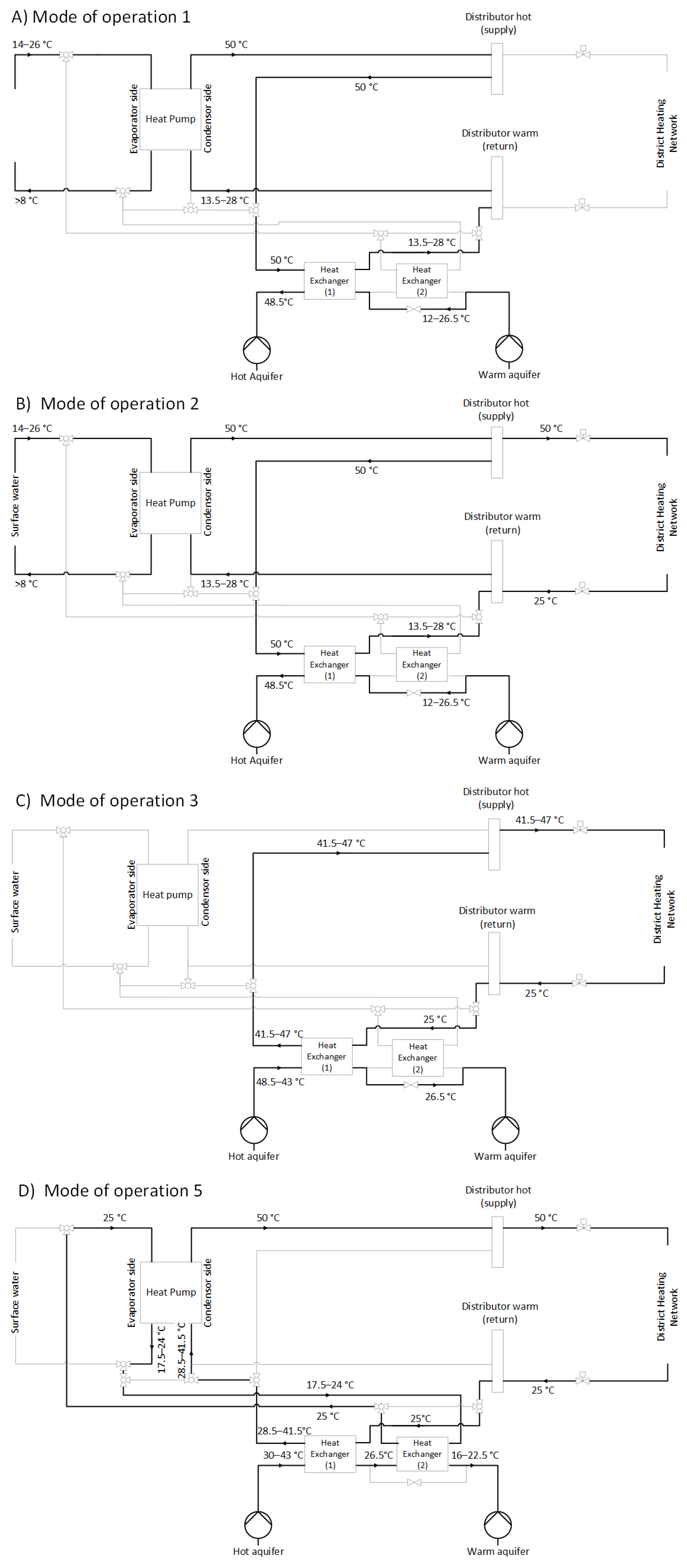
2.3.2. Modes of Operation for the Heat Pump and HT-ATES

The heating system has different modes of operation defined in the model, depending on the situation. In the explanation, we have chosen a heat pump condenser temperature of 50 °C and heat delivery via a district heating network (DHN) with a minimum of 40 °C. Schemes for a heat pump condenser temperature of 65 °C are given in the Supplementary Information. There are five possible modes of operation:

• Heat production and storage in the HT-ATES (no heat demand)
  In this mode of operation, heat is produced with surface water (14–26 °C) as input during the summer months (see Figure 3A). Heat is injected into the hot aquifer at 48.5 °C (assumed 1.5 °C loss over the heat exchanger).
• Simultaneous heat production and delivery
  If there is a heat demand at a time when the heat pump is producing heat (during summer), the heat demand is fulfilled directly from the heat pump (50 °C) via the hot distributor (see Figure 3B). After fulfilling the heat demand, the remainder of the heat is injected into the hot aquifer at 48.5 °C.
• Heat delivery from the HT-ATES above the inlet temperature of the district heating network (hot well > 43 °C)
  In the period from October–April (approximately), the heat pump is not able to produce heat with surface water as the surface water temperature is too low (<14 °C). Heat demand from the multi-energy system is now fulfilled by extracting heat from the hot aquifer of the HT-ATES system (see Figure 3C). Water from the hot well (43–48.5 °C) is extracted and exchanged with the return flow from the DHN (25 °C) and subsequently injected into the warm well (at 26.5 °C). The heat supply flow of the DHN is heated to 41.5–47 °C.
• HT-ATES is shut off. (Hot well under threshold temperature < 43 °C)
  In this mode of operation, the temperature of the hot aquifer has dropped below the threshold temperature (43 °C) to guarantee heat delivery at 40 °C. The HT-ATES system is now shut off and cannot be used to fulfil the heat demand of the multi-energy system.
  In this case, heat must be delivered from another (external) source, such as a peak boiler or a sustainable heat source. This is not included in this analysis.

For this study, we added an extra mode of operation to prolong the heat delivery from the HT-ATES system and to assess its effect on the efficiency of the heat production system and the heat production costs.

5.

HT-ATES feeds heat pump mode; heat delivery from the HT-ATES with alternative threshold temperature (hot well temperature between 30 °C and 43 °C)

To prolong heat delivery from the HT-ATES system, we designed an extra mode of operation for the heat pump and HT-ATES. In this mode of operation, the heat delivery from the HT-ATES continues when the temperature of the hot well is below 43 °C but above 30 °C. This is possible because of additional heat exchange with the HT-ATES in combination with a heat lift by the heat pump (see Figure 3D). First, the return flow of the DHN is exchanged with water from the hot well (30–43 °C) and thereby the return flow is heated to 28.5–41.5 °C. This already heated return flow of the DHN is then fed to the condenser side of the heat pump and raised to 50 °C. The flow from the hot aquifer is thus first exchanged with the return flow of the DHN, which results in a temperature of 26.5 °C. Then, the same flow is led to a second heat exchanger, to extract more heat by a (closed) loop that is connected to the evaporator side of the heat pump (inlet temperature of 25 °C). The return flow from the evaporator side of the heat pump is then finally exchanged with the flow that is injected in the warm well (at 16–22.5 °C). In this way, the heat from the hot well is exchanged in two stages before being injected into the warm well, making the heat exchange more efficient. Moreover, the injection temperature in the warm well is decreased, creating a larger ΔT between the wells which could be beneficial for the HT-ATES efficiency. The electricity demand of the heat pump in this mode is retrieved directly from local RES (renewable energy systems) when possible, or from the grid when no electricity from local RES is available.

2.4. Scenarios

The goal of this study is to identify methods for integration and control of a HT-ATES within a multi-energy system, as well as assess how these methods affect the performance of the energy system. In Section 2.3, we have introduced an additional mode of operation for the heat pump/HT-ATES system. We hypothesise that this mode of operation prolongs heat delivery from the hot well and could increase the overall performance of the heat pump/HT-ATES system. Therefore, we have selected ten scenarios (

Table 3. Overview of scenarios.

	Heat Pump Condenser Temperature	HT-ATES Threshold Temperature	Heat Pump Size
65|43|2	65 °C	43 °C	2 MWel
50|43|2	50 °C	43 °C	2 MWel
65|30|2	65 °C	30 °C	2 MWel
50|30|2	50 °C	30 °C	2 MWel
65|43|1.5	65 °C	43 °C	1.5 MWel
50|43|1.5	50 °C	43 °C	1.5 MWel
65|30|1.5	65 °C	30 °C	1.5 MWel
50|30|1.5	50 °C	30 °C	1.5 MWel
65|30|1	65 °C	30 °C	1 MWel
50|30|1	50 °C	30 °C	1 MWel

) to examine this hypothesis, as well as obtain general insights on how the HT-ATES system performs within the multi-energy system.

The heat demand and heat delivery temperature are kept constant for all scenarios. The amount of heat that should be provided to the neighbourhood houses is 55.2 TJ per year at a temperature of at least 40 °C. We have chosen to vary the condenser temperature, the threshold temperature (HT-ATES feeds heat pump mode) and the size of the heat pump. Table 3 gives an overview of the ten scenarios that are investigated in this study. The description code is built up as: condenser temperature|HT-ATES threshold temperature|heat pump size.

We compare two condenser temperatures because we hope to learn more about their actual effects on heat delivery, recovery efficiency and costs. We know that a higher condenser temperature of 65 °C leads to a lower COP of the heat pump compared to 50 °C, decreasing the amount of energy that can be stored with a given heat pump size. Additionally, the heat pump will be more expensive at a higher condenser temperature and more heat loss can occur at a higher storage temperature. On the other hand, storage at 65 °C leads to a smaller storage volume for the HT-ATES system, which saves costs and space. By comparing scenarios with both condenser temperatures, we obtain more insight into the combined result of these contradictory effects on the chosen performance parameters.

To ensure heat delivery at 40 °C, the threshold value for the hot well is set at 43 °C. In Section 2.3, we introduced an HT-ATES feeds heat pump mode that allows a lower threshold temperature of the hot well of 30 °C, as the heat pump is then used for an extra temperature lift. Scenarios 65|30|2, 65|30|1.5, 50|30|2 and the 50|30|1.5 will give insight into the effects of including this HT-ATES feeds heat pump mode, and can be compared to their respective twins where the HT-ATES feeds heat pump mode is not used and the threshold temperature is set at 43 °C.

Lastly, we investigate the effect of different heat pump sizes. A smaller heat pump will save costs, but it should be large enough for the HT-ATES system to provide sufficient heat in winter. We hypothesise that the scenarios with an extra heat pump mode lead to a more efficient HT-ATES system, which could imply that the amount of heat stored in the HT-ATES could be reduced. For a good comparison, we included scenarios with a 2 MW_el, 1.5 MW_el and 1 MW_el heat pump. We expect the 1 MW_el heat pump to be too small to fulfil the heat demand of the neighbourhood in the multi-energy system (55.2 TJ/y). With an average COP of 4 and approximately five months of heat production, a maximum of 51.8 TJ/y could be stored with a 1 MW_el heat pump, which is less than the heat demand of the neighbourhood (55.2 TJ/y). However, to investigate the effect of a relatively small heat pump on the HT-ATES system, we included two scenarios with a 1MW_el heat pump, both with a lower (30 °C) threshold temperature.

2.5. Assessment Framework

2.5.1. Fulfilment of Heat Demand

The main goal of the combined heat pump and HT-ATES system is to fulfil the heat demand of the neighbourhood in the multi-energy system in a reliable and affordable way. To fulfil the heat demand at a certain moment, there are multiple options. In our system, we first check if the heat demand can be fulfilled by direct heat production, which mainly happens during summer. Next, it is checked if the heat demand can be fulfilled by the HT-ATES system, which mostly happens in the winter season. If the HT-ATES feeds heat pump mode (see Section 2.3.2) is switched on, it is possible to increase the temperature of the HT-ATES with the heat pump, and the heat demand is fulfilled by the HT-ATES system with some additional electricity use. Lastly, if the temperature of the hot aquifer is below the set threshold temperature (43 °C or 30 °C in our case), the HT-ATES system will not be used for heat production. In this case, an external source of heat is necessary. This external source is not defined in this paper, but could, for example, be a peak gas boiler, or a renewable option.

In the first few years of operation, it is likely that the HT-ATES system has not yet stored enough heat to ensure continuous heat delivery throughout the year. However, the goal would be to reach continuous operation within a few years, so no external heat source is necessary and the heat pump-HT-ATES system can function independently.

Because the heat pump can work on 100% renewable electricity with surface water as a source, there are no direct GHG emissions of the system if it operates independently from an external source. Energy use during production and recycling of system components is not taken into account here. The GHG emissions of the external heat source are not taken into account in this study as we do not define a particular heat source.

2.5.2. HT-ATES Performance

The performance of the HT-ATES system is assessed with two main parameters, the well recovery efficiency of stored energy and the volume balance between the wells.

Regarding the recovery efficiency, we use three different indicators that give insight into the efficiency of the heat system as part of the multi-energy system. The performance of the HT-ATES system is calculated in terms of hot well recovery efficiency, warm well recovery efficiency and system recovery efficiency. For each indicator, a separate ΔT is used, see below. The average recovery efficiency (η) over the total run period (10 years) is calculated and analysed in the results section.

$$\eta =\frac{{{\displaystyle \sum }}_0^{10y} \Delta T ·V_{out ·} c_w}{{{\displaystyle \sum }}_0^{10y }\Delta T ·V_{in ·} c_w}$$

(5)

$$\Delta T_{system}={\widehat{T}}_{hot}-{\widehat{T}}_{warm}$$

(6)

$$\Delta T_{hot well}={\widehat{T}}_{hot}-T_{amb}$$

(7)

$$\Delta T_{warm well}={\widehat{T}}_{warm}-T_{amb}$$

(8)

T_hot and T_warm are the temperatures of the hot and warm well (in °C) per day, v_in and v_out are the flows in or out of the hot well (m³/h), and c_w is the heat capacity of water (4180 kJ/K/m³). T_ambient is the ambient background temperature of the aquifer (12 °C). Depending on the ΔT applied in Formula (5), either the system recovery efficiency (6), hot well recovery efficiency (7), or warm well recovery efficiency (8) is calculated.

Secondly, the volume balance ratio (r_VB) between the hot and warm wells is calculated as described by Beernink et al. (2019) [48]:

$$r_{VB}=\frac{V_{heat,storage}-V_{heat,production}}{V_{heat,storage}+V_{heat,production}}$$

(9)

where V_heat,storage is the yearly total storage volume (m³) and V_{heat,production} is the yearly total production volume (m³). Here, a positive ratio means that more volume is used to store heat in the hot well. Therefore, this also means that less volume is stored in the warm wells. Oppositely, a negative ratio means that more volume is stored in the warm wells.

2.5.3. MES Performance

For improved integration of HT-ATES within a multi-energy system, it is relevant to know the efficiency of the MES as a whole, under varying modes of HT-ATES integration. This indicator gives insight into the final efficiency by which the heat is delivered from the MES to the houses. Thus, this parameter is the amount of total delivered energy (heat) to the neighbourhood divided by the used total energy (electricity) for heat production:

$${\eta }_{MES}=\frac{E{n}_{del, 10y avg }}{CO{P}_{10y avg}·E{l}_{dem, 10y avg}}$$

(10)

With η_MES as the MES efficiency, En_{del,10 y avg} is the average amount of delivered heat to the neighbourhood (in TJ/year over the first ten years), which can thus be lower than the actual heat demand. COP_{10 y avg} is the average COP of the heat pump over the run time (10 years), and El_{dem,10 y avg} is the average electricity demand of the total heat system over the run time (10 years).

It includes the efficiency of both directly produced as well as stored heat and heat loss in the district heating network. In case a certain system design is not able to provide the total heat demand, this is corrected for by only taking the delivered heat into account and not the total heat demand of the neighbourhood. The part of the heat that must be delivered from an external source is thus not taken into account by this parameter. The MES efficiency purely gives the efficiency of heat delivery of the MES including a heat pump and HT-ATES system, without other sources.

2.5.4. Economic Analysis/Levelized Cost of Energy

We determine the levelized costs of heat production (LCOE) in €/GJ, including the costs for heat storage, and excluding the heat delivery (district heating network), according to:

$$LCO{E}_{heat}=\frac{{\displaystyle \sum }\alpha ·CAPE{X}_i+OPE{X}_i+E_{cos{t}_i}}{Q_{heat, delivered}}$$

(11)

in which:

$$\alpha =\frac{r}{1-{\left(1+r\right)}^{-L_i}}$$

(12)

where α is the capital recovery factor (no unit), representing a fraction of the total CAPEX costs depending on the yearly depreciation. r is the discount rate (as a fraction of 1) and L_i is the lifetime of a system component i. The CAPEX_i are the total capital expenditures for a particular system component i, such as the heat pump, heat exchanger or HT-ATES wells. OPEX_i are the operational expenditures and maintenance in €/year for a system component i, expressed as a percentage of the CAPEX. E_cost,i are the average (in this publication, for 10 years) electricity costs for the heat system (in €/year). These costs are thus only for the modelled heat system, and not for any external source that might be necessary to fulfil the total heat demand. Q_{heat,delivered} is the part of the heat demand delivered by the multi-energy system with HT-ATES in GJ/year. We thus only take into account the heat that can actually be delivered by the multi-energy system with HT-ATES and not by an external source. This ensures a fair LCOE comparison between different scenarios.

Cost data is given in

Table 4. Investment and operational costs for HT-ATES components.

System Component	CAPEX (in €)	OPEX (%)	Lifetime
Aquifers and equipment a	(75,860 × ln(kWth/6.69) − 115,000) × 1.25	4%	30
Heat exchanger b	1500 × √kWth × 1.1	2%	20
Heat pump—65 °C condenser temp. c	600 €/kWth	1%	20
Heat pump—50 °C condenser temp. c	400 €/kWth	1%	20

^a Formula was originally for ATES systems [50], and is adapted for HT-ATES by multiplying with 1.25, because at higher temperatures more expensive materials have to be used. ^b Costs data based on supplier data for ATES systems, multiplied by 1.1 for higher temperatures (HT-ATES). ^c Costs estimation based on different sources [41,51] in combination with supplier data. Heat pump size in MW_th is calculated by multiplying the electrical power (MW_el) with the average COP of the heat pump in that scenario.

. A discount rate (r) of 6% (0.06) is applied, and electricity costs are set at 60 €/MWh_e based on CBS data for non-households with an electricity demand of >70,000 MWh_e in 2019 [49], and is similar to Wesselink et al. 2018 [22].

Lastly, the electricity use of the heat pump is calculated, averaged over the run period (here 10 years).

3. Results

In the previous section, we described the models, the coupling of the models and the scenarios that are used as input for the coupled model infrastructure. In this section, we describe the results of the scenario model runs assessed on the heat fulfilment by the (HT-ATES) system to the neighbourhood, the performance of the HT-ATES, the differences in costs (LCOE) between scenarios, and finally we combine these results in an overall analysis of the performance.

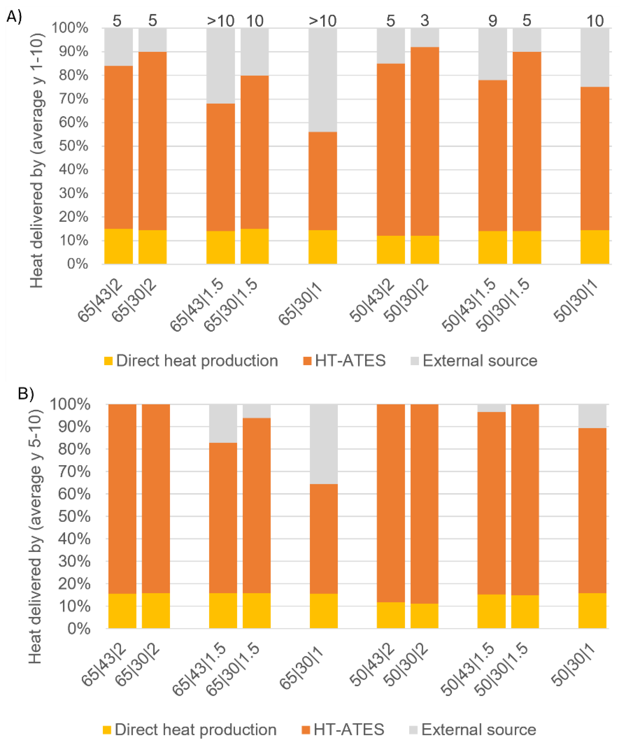
3.1. Fulfillment of Heat Demand with HT-ATES

Simulation results show that in all cases, 12–14% of the heat demand in summer is delivered to the neighbourhood directly by the heat pump for all scenarios (Figure 4) during the ten-year simulation (A) and the last five years of the simulation (B). This percentage is the same for each scenario because the net demand is the same and in all cases, the heat pump capacity is much larger than the heat demand in summer, when the heat pump produces heat that otherwise would be stored in the HT-ATES.

The simulation results show that at the heat delivered from the HT-ATES, a distinction is made between scenarios that are able to reach heat delivery by the HT-ATES system within five years, and scenarios that take longer to reach 100% delivery of demand by the heat pump and HT-ATES system. In scenarios that take longer than five years to reach 100% delivery, the HT-ATES system is shut off for >20% of the time, which negatively influences the amount of heat delivered from the HT-ATES system (40–65%). The other scenarios that reach a stable heat supply within five years have 70–80% of the heat demand delivered from the HT-ATES system. In Figure 4B, the origin of the heat delivered during the last five years of operation of the heat pump-HT-ATES system are shown. Five scenarios can operate independently of an external source after an initial start-up period.

For this case study, we show that the addition of a HT-ATES to a multi-energy system with power-to-heat results in >90% fulfilment of the heat demand during the first 10 years of operation, while after 3–5 years, the combined system can supply the full heat demand of the neighbourhood in the multi-energy system sustainably.

The HT-ATES feeds heat pump mode of operation allows a lower threshold temperature. As a result, the HT-ATES system can be operated longer during winter. Hence, with a 2 MW_el heat pump, the amount of heat provided from the HT-ATES is increased by 6–7% when using the HT-ATES feeds heat pump mode (see Figure 4A). When specifically comparing the scenarios at 50 °C condenser temperature (see 50|43|2 and 50|30|2 in Figure 4A), the HT-ATES feeds heat pump mode decreases the time needed to reach 100% heat delivery from 5 to 3 years. This positive effect of the HT-ATES feeds heat pump mode is even more pronounced with a 1.5 MW_el heat pump and leads to 9–11% more heat delivery from the HT-ATES system.

For the 65 °C and the 1MW_el and 1.5 MW_el heat pump scenarios, it is not possible to reach 100% heat delivery in 10 years. Without the HT-ATES feeds heat pump mode, an external heat source is still necessary after 10 years of operation (see 65|43|1.5 and 65|30|1.5 in Figure 4A).

At 50 °C, the HT-ATES feeds heat pump mode is able to reduce the time it takes to reach stable operation to five years, compared to nine years for a scenario without the HT-ATES feeds heat pump mode (see 50|43|1.5 and 50|30|1.5 in Figure 4A). Thus, the HT-ATES feeds heat pump mode makes it possible to create a reliable HT-ATES system with a smaller heat pump (1.5 MW_el vs. 2 MW_el) at 50 °C condenser temperature.

The amount of electricity necessary for this mode comes from local RES when possible, or from the grid otherwise. In Figure 5, the electricity demand for heat production is shown over time in relation to the heat demand. This graph makes it clear that the electricity demand for the extra mode of operation is small in relation to the total electricity demand of the HT-ATES system. In all scenarios, it is never more than 2–6% of the total electricity demand of the HT-ATES system (6% for the 65|30|1.5 scenario in Figure 5). This small amount of electricity used in winter decreases the utilization of an external heat source for fulfilment of heat demand by 6–12%, depending on the scenario (12% for the 65|30|1.5 scenario). Furthermore, Figure 5 clearly shows the temporal decoupling of heat production and demand made possible by the integration of HT-ATES in the MES.

3.2. HT-ATES Performance

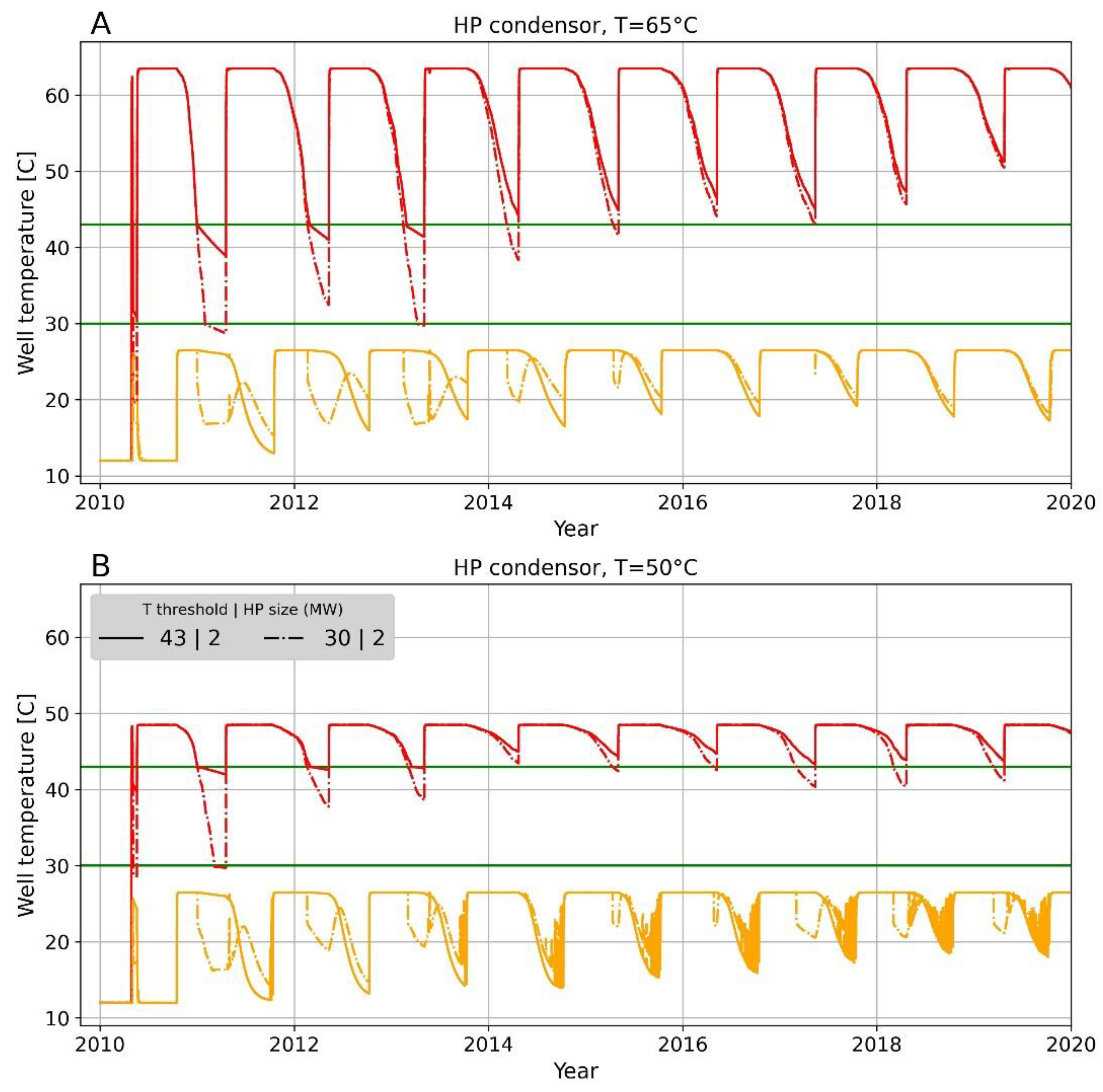
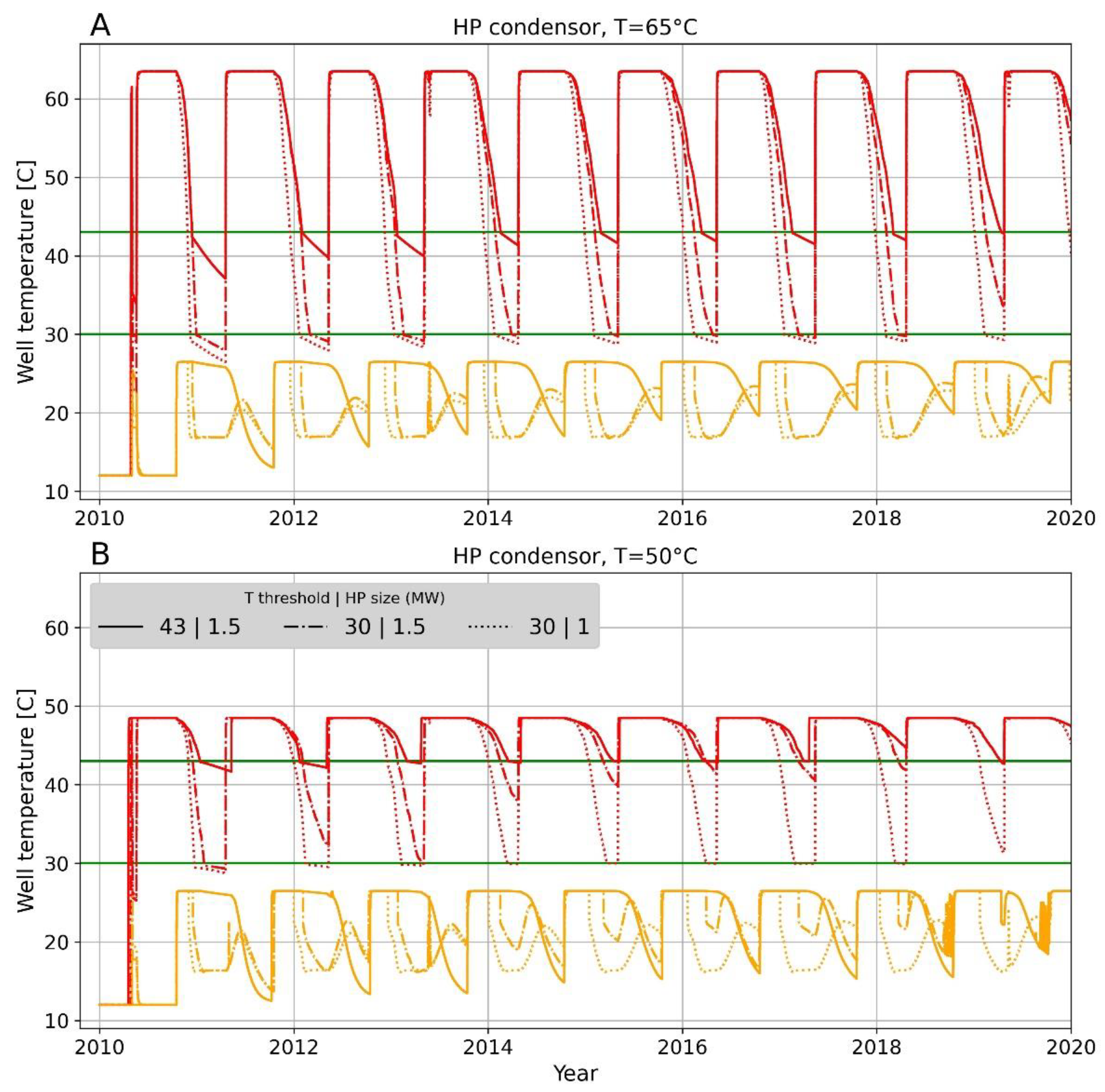
3.2.1. Well Temperature Development

Results show that the fulfilment of the heating demand by the HT-ATES system varied significantly between the 10 scenarios (Figure 4), to a large extent as a result of the varying performance of the HT-ATES system. The HT-ATES system cannot supply the entire demand if the threshold temperature is reached during heat extraction from the hot well. Figure 6 shows the well temperature over time of the relatively large 2 MW_el heat pump size scenarios. The hot well temperature drops below the threshold temperature during recovery in the first years. After year 4, the hot well temperature always stays above the threshold temperature, both for the T_threshold = 43 °C and the HT-ATES feeds heat pump mode (T_threshold = 30 °C). The effect of the HT-ATES feeds heat pump mode is visible as a sharp drop in warm well temperature when the hot well temperature drops below the first threshold of T = 43 °C. For the 65 °C storage temperature, the HT-ATES feeds heat pump mode is no longer activated after the system has sufficiently warmed up after the first years, as shown in Figure 6A. For the 50 °C storage scenarios (Figure 6B), the HT-ATES feeds heat pump mode is active for most of the modelled years, because the hot well temperature often drops below the threshold of 43 °C at the end of extraction season. This is also visible in the warm well temperature of this scenario in Figure 6B; the warm well temperature drops once the HT-ATES feeds heat pump mode becomes active, which results in a very irregular warm well temperature pattern.

For the smaller heat pump scenarios (1.5 and 1 MW_el), the temperature in the hot and warm wells is presented in Figure 7. Here we observe the same behaviour, but the temperature drops in both the hot and the warm wells are stronger. Hence, for these smaller heat pump capacity scenarios, less heat is stored compared to a 2 MW_el heat pump, resulting in a more depleted heat storage at the end of the extraction season. As a result, the threshold temperature of 43 °C is reached for both the 65 °C scenarios and the 50 °C scenarios in almost all years. However, at the end of the simulated period, we see that higher temperatures are maintained and the threshold temperature is reached less often. This indicates that the losses of previous years have created a shell with elevated temperature around the stored volume over time. As a consequence, the heat loss decreases and the system moves towards an equilibrium situation.

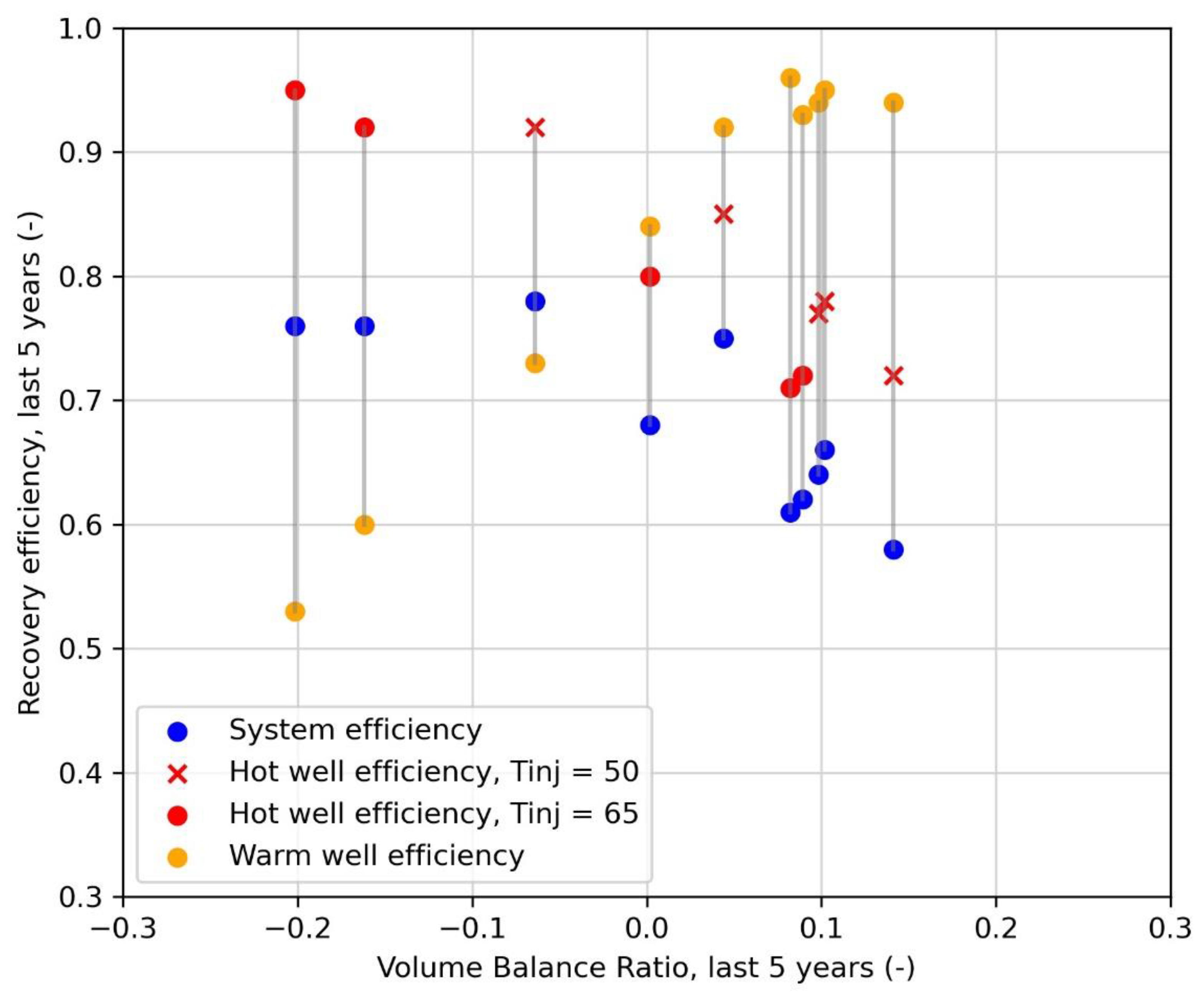
3.2.2. HT-ATES Performance Results

The hot well, warm well and system recovery efficiency are presented in

Table 5. Ten-year average HT-ATES performance results. The amount of stored energy is mainly determined by the size of the heat pump and the temperature levels. This subsequently results in different amounts of stored volumes and recovery efficiencies. The scenario name abbreviation consists of: condenser temperature|HT-ATES threshold temperature|heat pump size.

Scenario	Vhot Injection 10y Average (103 m3/y)	Vhot Extraction 10y Average (103 m3/y)	Volume Balance Ratio (rVB)	Hot Well Recovery Efficiency 10y Average (-)	Warm Well Recovery Efficiency 10y Average (-)	HT-ATES Heat Delivered 10y Total (Endel,10 y avg in TJ)	HT-ATES Heat Stored 10y Total (TJ)	HT-ATES System Recovery Efficiency 10y Average (-)	MES Efficiency 10y Average (ηMES )
65|43|2	446	339	0.14	0.64	0.88	413	778	0.53	0.53
65|30|2	450	397	0.06	0.69	0.85	445	780	0.57	0.56
65|43|1.5	330	282	0.08	0.70	0.82	322	569	0.57	0.57
65|30|1.5	315	389	−0.10	0.83	0.59	377	568	0.66	0.63
65|30|1	193	259	−0.15	0.86	0.51	239	354	0.68	0.64
50|43|2	774	509	0.21	0.63	0.92	436	900	0.48	0.48
50|30|2	736	570	0.13	0.71	0.89	480	838	0.57	0.55
50|43|1.5	692	450	0.21	0.62	0.90	381	810	0.47	0.48
50|30|1.5	680	540	0.11	0.71	0.87	448	785	0.57	0.55
50|30|1	432	441	−0.01	0.83	0.69	351	522	0.67	0.61

.

In the previous section, we showed that the heat that is delivered by the multi-energy system is influenced strongly by the size of the heat pump. With a large heat pump size, more energy is stored in the subsurface in summer, which results in more energy that is recovered in winter. Table 5 shows that, while this might feel counter-intuitive, the system recovery efficiency is lowest (50–55%) for the scenario where most heat is provided to the multi-energy system (largest heat pump scenarios) and vice versa. Because the amount of stored energy varies between the scenarios, the delivery of heat from the HT-ATES system cannot be directly coupled to the recovery efficiency of the HT-ATES system.

In the large heat pump scenarios, more volume is stored in summer than required (and thus recovered) in winter, resulting in low recovery efficiencies. Oppositely, for the small heat pump scenarios, more volume is extracted in winter compared to what was stored in summer. The balance between these two volume flows, the volume balance ratio (r_VB) varies from −0.15 for small heat pump scenarios to 0.21 for the large heat pump scenarios (Table 5).

In Figure 8, the recovery efficiency and r_VB during the last five years of simulation are shown. The r_VB has an opposite effect on the hot and the warm well efficiency. For the hot well, a negative r_VB means that relatively large amounts of water is extracted, compared to what was initially injected, resulting in high recovery efficiency. The opposite is true for positive r_VB.

The system recovery efficiency is a result of the recovery efficiency of the hot and the warm well. However, the hot well has a stronger influence, compared to the warm well, because relatively more heat is stored in this side of the system. Consequently, the highest system recovery efficiency is observed for the highest hot well recovery efficiencies at negative r_VB. However, for the lowest r_VB ratios, the system recovery efficiency stops increasing because the warm well recovery decrease has a stronger effect compared to the hot well recovery efficiency increase. It thus seems that maximal system recovery is obtained at slightly negative r_VB.

The recovery efficiency is not only influenced by the volume balance ratio; the storage temperature affects the recovery efficiency as well. For higher storage temperature, more losses due to buoyancy flow occur, resulting in lower recovery efficiency. This is clearly visible for the scenario operating in volume balance (last five years) in Figure 8. Here, the warm well recovery efficiency is higher compared to the hot well recovery efficiency. Moreover, we observe two linear relationships for the hot well efficiencies, corresponding to the two varied storage temperatures, which is due to higher energy losses during storage for the 65 °C storage scenarios. Due to the limited difference in storage temperatures (65 °C vs. 50 °C) and the strong effect of volume balance, the recovery efficiency is dominated by the volume balance ratio for the simulated scenarios.

The system recovery efficiency of the HT-ATES only indirectly provides insight into the amount of heat that is delivered to the multi-energy system, because this depends on the absolute amount of energy that is actually stored in the HT-ATES system. The largest heat pump scenarios can store and deliver most heat, but they do this with a relatively small system recovery efficiency, shown in Figure 9. Consequently, this means that a relatively high amount of the stored heat is lost to the subsurface. Additionally, we observe here that for equal heat pump size, the 50 °C scenarios can provide more heat, with a lower system recovery efficiency. This is caused by the fact that more heat is stored for the 50 °C scenario (higher COP of heat pump) and that less heat is lost during storage due to the lower storage temperature and larger storage volume.

To get more direct insight into the actual efficiency of the delivered heat within the MES, we have included the system delivery efficiency in the calculations (see Table 5). The system delivery efficiency of the MES is similar (1–2% lower) to the system recovery efficiency of the HT-ATES for most scenarios. This outcome indicates that heat loss in the district heating network and the direct heat production and delivery more or less outweigh each other in these scenarios. Three scenarios that take longer than eight years to reach 100% delivery and have a negative r_VB (65|30|1.5, 65|30|1 and 50|30|1) have a slightly lower MES efficiency (3–6%) than HT-ATES system recovery efficiency. Still, the same trend is observed that scenarios with a small heat pump have a high MES efficiency, but a relatively low amount of heat delivered, and vice versa.

The influence of the HT-ATES feeds heat pump mode when recovery temperatures reach the threshold is observed in Figure 9. For the four scenarios for which both the normal and the extra mode of operation were simulated, we observe that both the absolute amount of energy that can be delivered to the multi-energy system and the system recovery efficiency strongly increase. The HT-ATES feeds heat pump mode thus has a positive impact on the performance of the HT-ATES, resulting in a higher recovery efficiency of the system (4–10% depending on the scenario) which increases the amount of heat delivered (in TJ) to the houses (7–15% depending on the scenario).

In Figure 9, the optimal scenario regarding heat delivery is the 50|30|2 scenario, because most heat is delivered (difference of 25 TJ), while the same system recovery efficiency is observed as the 50|30|1.5 and 65|30|2 scenarios.

3.3. LCOE of Heat Production and Storage

The levelized costs of energy (in this case heat) in €/GJ are shown in

Table 6. Energetic and financial performance of the heat production and storage system as part of a multi-energy system. The % of heat delivered by the HT-ATES/heat pump is the sum of the yellow and orange bars in Figure 4. The scenario name abbreviation consists of: condenser temperature|HT-ATES threshold temperature|heat pump size.

Scenario	Average COP Heat Pump (COP10 y avg)	Max. Capacity Infiltrated (MWth)	Max. Capacity Delivered (MWth)	Amount of Doublets	Average Electricity Demand—10y Average (Eldem,10 y avg in TJ/y)	% of Heat Demand Delivered by the HT-ATES/Heat Pump	Heat Production Costs (LCOE in €/GJ)
65|43|2 *	4	8.8	11.7	6	21.8	84%	19.6
65|30|2 *	4	8.8	11.7	6	22.2	90%	18.6
65|43|1.5	4	6.5	10	6	16.5	68%	18.5
65|30|1.5	4	6.5	11	7	17.7	80%	16.6
65|30|1	4	4.3	8.3	6	12.0	56%	16.7
50|43|2 *	5.5	12.6	11.7	7	17.6	85%	17.1
50|30|2 *	5.5	12.6	11.7	7	16.7	92%	15.7
50|43|1.5	5.5	9.4	11.8	8	16.3	78%	15.5
50|30|1.5 *	5.5	9.5	11.6	8	16.3	90%	13.8
50|30|1	5.6	6.2	10.9	7	12.6	75%	12.2

* The * added to the scenario code indicates that the HT-ATES can deliver 100% of the heat to the multi-energy system within the first five years.

. All scenarios with a 50 °C condenser temperature have a higher LCOE (2.5–4.5 €/GJ or 11–18%) than at 65 °C condenser temperature with the same heat pump size. An important reason is the higher COP for the 50 °C scenarios, which results in more heat injection in the HT-ATES with the same heat pump size. The difference in COP is proportional to the difference in Carnot efficiency based on the extra temperature lift when the heat pump condenser temperature is raised to 65 °C instead of 50 °C. This means that it is 30% more efficient to produce heat from surface water at 50 °C (average COP = 5.5) than at 65 °C (average COP = 4). Moreover, the heat pump investment costs per kW_th are higher for 65 °C (600 €/kW_th) than for 50 °C condenser temperature (400 €/kW_th). On the other hand, this cost difference is almost cancelled out as the COP is higher at 50 °C, resulting in a higher thermal heat pump capacity for the same electrical heat pump capacity. Eventually, the investment costs for the heat pump are slightly lower (around 6%) with 50 °C condenser temperature. The investments for the HT-ATES depend on the required capacity and with that the number of doublets (shown in Table 6). There is an increase of one doublet required at 50 °C vs. 65 °C condenser temperature, as the capacity delivered from the HT-ATES is quite similar over all scenarios, resulting in limited variations in the HT-ATES investment costs across the scenarios. The main decrease in costs between 50 °C and 65 °C condenser temperature is caused by the lower electricity demand (because of higher COP) at 50 °C vs. 65 °C.

Next to the condenser temperature, the HT-ATES feeds heat pump mode has an impact on the LCOE. The differences in results between 65|43|2 and 65|30|2, as well as the 50|43|2 and 50|30|2 scenarios illustrate this, as the only difference here is the extra mode of operation. In both cases with the additional mode of operation, there is an increase in costs for an additional heat exchanger, but a decrease in electricity costs while the amount of delivered heat increases. For the 65 °C condenser temperature, the electricity costs increase by 2%, while 6% more heat is delivered from the heat pump/HT-ATES system, which leads to a reduction of 1.0 €/GJ for the LCOE; while at 50 °C condenser temperature, the HT-ATES feeds heat pump mode leads to a decrease in electricity costs of 5%, and 7% more heat delivered, resulting in a total LCOE decrease of 1.4 €/GJ.

The HT-ATES feeds heat pump mode thus results in extra heat delivered at limited extra costs, hence the low LCOE for these scenarios. With a smaller heat pump size of 1.5 MW_el, the LCOE decreases further. For the 65 °C scenarios, the electricity demand does significantly decrease as well, although the % of heat demand delivered decreases with a smaller heat pump. Still, a reduction of 1.1 €/GJ is realized compared to a 2 MW_el heat pump with an LCOE of 18.5 €/GJ. The cost reduction is further enhanced by the HT-ATES feeds heat pump mode with 12% more heat delivery resulting in an LCOE of 16.6 €/GJ. For a 50 °C condenser temperature, the same effects are visible, although in this case, the HT-ATES feeds heat pump mode does not lead to an increase in electricity demand, but raises the heat demand delivered to 90%, which is almost similar to the 50|30|2 scenario, but with a smaller heat pump (1.5 MW_el vs. 2 MW_el). In this scenario (50|30|1.5), the LCOE is 13.8 €/GJ, which is 1.7 €/GJ lower than without the HT-ATES feeds heat pump mode.

A 1 MW_el heat pump with a 65 °C condenser temperature (65|30|1) does not lead to a further decrease in LCOE compared to a similar scenario with a 1.5 MW_el heat pump (65|30|1.5). The savings on heat pump investment and electricity costs thus do not compensate for the decrease in heat delivery (56% vs. 80%) by the heat pump/HT-ATES system.

Overall, the 50|30|1 scenario with a 1 MW_el heat pump has the lowest LCOE, with 75% of the heat demand delivered from the heat pump/HT-ATES system. The lower investment costs for the heat pump do make this scenario the most feasible. Furthermore, these results show that by installing a HT-ATES system, the heat pump size is not the determining factor for heat delivery anymore. As the HT-ATES is the main source of heat delivery during winter, the capacity of the HT-ATES system is more important than the size of the heat pump. HT-ATES systems thus help to reduce the size of the heat pump.

These results indicate a tipping point in heat pump size in relation to the amount of heat that can be delivered from the HT-ATES system to the multi-energy system. In the cases where the heat pump size is becoming a limiting factor, the positive effect of the extra mode of operation is most pronounced. The actual heat pump size tipping point will depend on the local conditions (maximum required heating power, temperature level) and thus vary per project. This analysis showed that for identifying the lowest LCOE scenario, it is worthwhile to identify this tipping point when a HT-ATES system in a multi-energy system is realized.

3.4. Overall Performance: An Integral View on Heat Delivery, System Efficiency and Costs

In this study, we considered several scenarios with varying heat pump designs and storage temperature levels and assessed how these variations impact the fulfilment of the neighbourhood heat demand, the performance of the HT-ATES system, and the costs of heat production including storage (LCOE). The overall performance of the varied scenarios is assessed here by combining all assessment criteria, as shown in Figure 10. Here, the arrows indicate the influence of the HT-ATES feeds heat pump mode compared to the normal operation mode. The most optimal system would have: 1. a large amount of delivered heat (y-axis); 2. a high HT-ATES system efficiency (x-axis); and 3. low LCOE (colour). The following observations stand out:

-

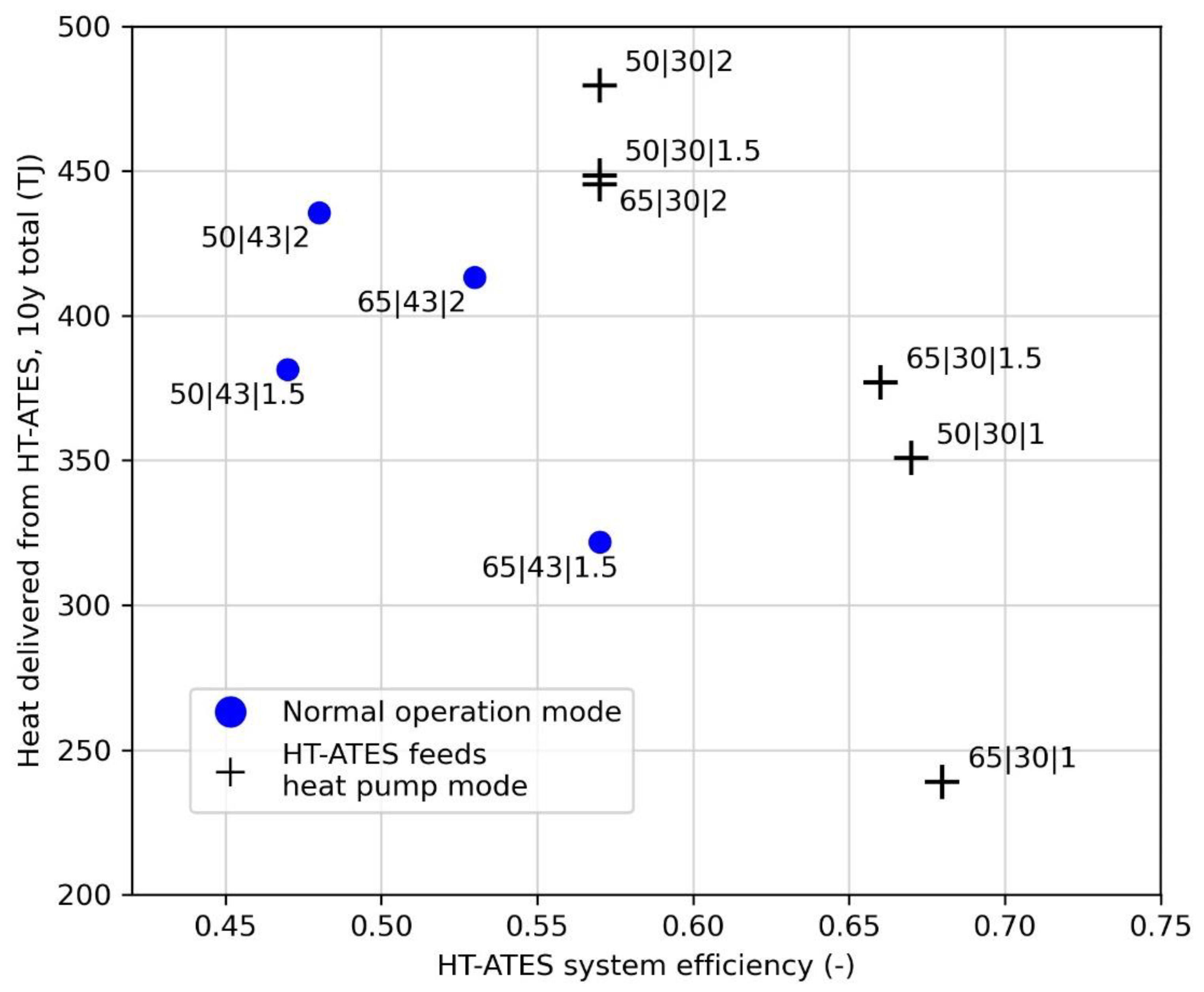
At a small heat pump size and a high storage temperature (65|30|1), a relatively small amount of the total heat demand can be delivered to the multi-energy system (0.56) and LCOE does not decrease compared to a 1.5 MW_el heat pump scenario (both around 16.6 €/GJ). However, decreasing the storage temperature to 50 °C has a large positive effect for this small heat pump scenario (50|30|1); the LCOE strongly decreases (16.7 to 12.2 €/GJ) and the delivered amount of heat increases to 75%.

-

Overall, the 50 °C storage temperature ensures lower costs and higher fulfilment of heat demand to the neighbourhood. This is probably caused because the heat pump is cheaper and more effective, which results in larger amounts of stored heat. This has a stronger effect than the increase in costs due to the needed number of wells.

-

For all scenarios, the HT-ATES system feeds heat pump mode (43 °C vs. 30 °C shut-off temperature) has a strong positive effect on all assessment criteria: the LCOE decreases, the fulfilment of heat demand increases, and the MES efficiency increases. Hence, this mode of operation has a high potential to be integrated into future HT-ATES systems. With only a small amount of electricity use in winter (not more than 2–6% of the total electricity use), the amount of heat delivered from the HT-ATES increases by 6–12%.

-

The most optimal scenario for this neighbourhood, based on all assessment criteria, is the 50|30|1.5 MW scenario. This scenario can provide 100% of the heat demand year-round to the neighbourhood within the first five years, while the LCOE is 13.8 €/GJ, the second cheapest system.

4. Discussion

4.1. The Functioning of a HT-ATES within a Multi-Energy System

We have shown that seasonal heat storage, HT-ATES, is crucial to be able to increase the amount of locally provided sustainable energy in a multi-energy system. Hence, HT-ATES is probably a better option for seasonal heat storage instead of the hot water storage tanks that are usually applied in a multi-energy system [12,14,15,19]. However, HT-ATES is not applicable everywhere, as it requires the presence of an aquifer.

The use of HT-ATES including the heat pump booster mode enables better utilisation of the stored heat, and with that, increases HT-ATES performance. We showed that this mode of operation has a high potential to be integrated into future HT-ATES systems, because the costs strongly decrease and HT-ATES performance increases, leading to an increase in local sustainable heat delivery.

The performance of the HT-ATES system is assessed via the recovery efficiency of heat from the HT-ATES system. The HT-ATES system recovery is determined by the recovery efficiency of heat from the hot and the warm well, which are strongly related to the volume (im)balance between the two wells. When the volume imbalance is negative (net extraction from the hot well), the recovery efficiency of the hot well increases and decreases at the warm well. However, the total amount of energy that can be provided to the MES can be larger than expected based on a simulation with a volume balance. For example, this could have a significant improvement for the recovery efficiency of HT-ATES wells that experience high heat losses during storage. Previous studies [31,52,53] evaluated the effect of several HT-ATES storage conditions on the recovery efficiency at V_in = V_out, and showed that energy losses can vary significantly. Therefore, it is recommended to analyse the combined effect of both varying storage conditions and the effect of volume (im)balance on recovery efficiency to get insight in the optimal combination of both factors for a given scenario.

In this study, we separately simulated the hot and warm wells of the HT-ATES systems. In reality, the wells will be placed next to each other, in such a way that positive interaction from the hot and warm wells is optimal. Previous studies showed that this leads to increased HT-ATES system performance [36].

4.2. The Impact of HT-ATES in a Multi-Energy System

In a multi-energy system with power-to-heat but without a HT-ATES, the heat pump size would be determined by the maximum peak in heat demand. By including a HT-ATES system in the multi-energy system, the heat demand and supply are mostly decoupled and the (peak) heat demand is delivered from the HT-ATES system during winter. The heat pump is employed in an optimal way by producing most of the heat in summer, the most likely time of abundance of (local) solar energy, but is also, to a small extent, employed in winter for the HT-ATES feeds heat pump mode when necessary.

Figure 11 shows the maximum capacity delivered to the heat users and the condenser capacity of the applied heat pump. The scenarios which end up in 100% heat delivery by the HT-ATES in the multi-energy system (*) indicate that the peak heating demand is 11.8 MW_th. For these scenarios, the ratio of the maximum demand and the applied condenser capacity shows how much smaller heat pump capacity can be installed to optimally utilise heat produced by power surplus. The 50|43|2 and 50|30|2 scenarios have a positive ratio, indicating the heat pump is over-dimensioned. From the 65|43|2, 65|30|2, 50|43|1.5 and the 50|30|1.5 scenario results, it is concluded that the heat pump can have a 21–25% smaller capacity than the actual peak heating demand. The other scenarios (not leading to 100% heat delivery) have ratios of 0.6–0.7, indicating that 25% lower heat pump capacity is the maximum. Besides a smaller capacity, the heat pump is employed both in summer to store the heat and in winter to provide additional heat when the HT-ATES heat production is not sufficient. This fosters year-round heat pump utilisation, although the energy use in winter is a fraction (<6%) of the total energy use of the HT-ATES system (see Figure 5). Thus, most energy demand is still during summer, with a likely oversupply of sustainable local electricity from PV.

The addition of HT-ATES in a power-to-heat MES affects the total yearly electricity use, and, the yearly distribution of electricity use, as energy demand and availability are decoupled. For a multi-energy system with power-to-heat without HT-ATES, all heat needs to be produced directly by the heat pump on demand, which can become a problem in winter because (a) the temperature of the heat source (canal) becomes too low to use, and (b) sustainable power to run the heat pump is not available. This results in the need for larger heat exchangers and the need for other sources of heat and associated costs, as well as a reduction in the use of local sustainable energy.

Following the basic heat pump dynamics, a simplified calculation for a multi-energy system with only direct heat production will result in a total average electricity use of 12.8 TJ/year with a 3.1 MW_el heat pump (assuming an average heat pump evaporator temperature of 8 °C, and 50 °C condenser temperature), with an electricity demand as shown in Figure 12. In the first 10 years of operation, a MES with HT-ATES will consume around 16–17 TJ/year of electricity and a maximum of 90% of the heat demand will be fulfilled. Yet, after the first two to four years of operation, the heat demand can be provided completely from the HT-ATES and the electricity demand of the system decreases. For example, in the case of the most optimal 50|30|1.5 scenario, the electricity demand in the 10th year of operation is 13.6 TJ. This is about 6% higher than a MES with direct heat production. The total electricity use thus slightly increases when HT-ATES is included. The total electricity use by the HT-ATES + HP system is influenced in two ways. Firstly, the source of heat (canal) is mainly harvested when its temperature is relatively high. This is favourable for the heat pump COP and results in relatively less electricity use. Secondly, more heat needs to be produced than the total yearly heat demand because a part of the produced heat will be lost during storage. Hence, the second effect is of slightly more influence on the total electricity demand in this study, for the first 10 years of operation. However, as pointed out in the previous section, the energy losses of HT-ATES systems, and thus their electricity use, may vary strongly for different HT-ATES storage conditions (e.g., storage volume, hydrogeological conditions). Consequently, under more favourable storage conditions, yearly electricity use of the MES may be lower compared to direct heat production.

More importantly, the integration of HT-ATES has a strong effect on the distribution of electricity use over the year. The electricity use is decoupled by the integration of HT-ATES, and the electricity use peak switches from winter to summer, following the availability of sustainable electricity by solar energy (Figure 12). Here, we compare the electricity use of a MES with and without HT-ATES. The electricity use of scenario 50|30|1.5 is compared to a reference system that uses a HP for direct heat production only.

Thus, the HT-ATES system enables the use of more sustainable and local electricity when available (in summer) and reduces the size of the heat pump compared to systems with direct heat production. The yearly electricity use slightly increases for the modelled scenarios in this study; however, this may change under more favourable HT-ATES storage conditions.

4.3. The LCOE Placed in Perspective

The LCOE for the different scenarios of heat pump size, condenser temperature and threshold temperature varies between 16.6–19.6 €/GJ for 65 °C heat pump condenser temperature, and between 12.2–17.1 €/GJ for 50 °C condenser temperature. Choosing a lower condenser temperature (50 °C instead of 65 °C) leads to lower costs as the COP of the heat pump is higher and the costs of the heat pump are assumed to be lower. However, exact cost curves of (large scale) heat pumps are not available, so the cost difference is not known exactly and needs further investigation. Additionally, at 50 °C condenser temperature, the total stored volume in the HT-ATES is approximately twice as large as at 65 °C, and therefore requires more hydraulic pumping for the injection and abstraction.

The costs of the assessed scenarios in this paper are comparable to the costs (20.5 €/GJ) that were determined by Wesselink et al. [22], who considered a HT-ATES system in combination with geothermal energy. In an overview of different HT-ATES feasibility studies, the LCOE of heat varied between 14.7–29.3 €/GJ, with larger systems (>350,000 m³) resulting in a LCOE below 20 €/GJ [54]. The LCOE calculated in this paper thus fits within the price range known for HT-ATES systems. Heat delivered by a gas boiler costs on average 10–12 €/GJ [49]. For the scenarios considered in this paper, calculated prices are higher with a minimum difference of 0.2–2.2 €/GJ (50|30|1). This gap could be bridged by an increase in the CO₂ price or subsidies on the installation or heat price of 100% renewable power-to-heat systems with HT-ATES. With a CO₂-price of 55.6 €/ton CO₂ and CO₂-emission factor of 35.97 kg CO₂/GJ of heat [55], the LCOE of a gas boiler would rise to 12–14 €/GJ, which would then fall in the same range as the 50|30|1 and 50|30|1.5 scenarios. At a CO₂-price of 100 €/tonne CO₂, the price range of heat from a natural gas boiler would rise to 13.6–15.6, increasing the feasibility of a HT-ATES system with power-to-heat further.

4.4. Prolonged Lifetime of the Multi-Energy System with HT-ATES

In this study, only the first ten years of operation of the HT-ATES have been simulated. The lifetime of the multi-energy system and HT-ATES is longer than ten years, and the results show that most scenarios can reach a 100% heat delivery within the first ten years of operation (see Figure 6 and Figure 7). After this time, the electricity demand is more representative compared to the first few years of operation as the system is still stabilizing and not able to provide the total heat demand. Hence, we performed an extra financial analysis assuming the electricity demand of the 10th year of operation would stay constant for the next 30 years of operation. This is a conservative estimation because the systems will most likely continue to improve in performance and system recovery efficiency over the years. On the other hand, we assumed that all systems would be able to provide the total heat demand of the neighbourhood after 10 years of operation, although we are not completely sure about this for i.e., scenario 65|43|1.5, 65|30|1.5, 65|30|1, and 50|30|1. The results can thus not be used to reliably compare the scenarios with each other, but give an idea of how the LCOE would develop over time. The results are shown in

Table 7. LCOE analysis with 30 years of operation of the heat pump/HT-ATES system.

	Heat Production Costs (LCOE) in €/GJ—10 Years	Heat Production Costs (LCOE) in €/GJ—30 Years
65|43|2	19.6	17.4
65|30|2	18.6	17.4
65|43|1.5	18.5	14.3
65|30|1.5	16.6	14.3
65|30|1	16.7	11.1
50|43|2	17.1	14.6
50|30|2	15.7	14.2
50|43|1.5	15.5	13.0
50|30|1.5	13.8	12.3
50|30|1	12.2	10.1

and show a reduction of 1.2–5.6 €/GJ, which is a reduction in LCOE of 4–28% and 13% on average. The LCOE presented in this paper are thus a conservative estimation and will be significantly lower when considering a lifetime of 30 years, which would be further enhanced when a reduction in electricity consumption is taken into account as well.

5. Conclusions

In this study, it is shown that with the novel integration of a HT-ATES system to a multi-energy system, it is possible to provide >90% of the heat demand during the first ten years of operation, and supply the full heat demand after 3–5 years. The system recovery efficiency of the HT-ATES system was 50–70% depending on the system design chosen. By including a HT-ATES system in a multi-energy system, the size of the heat pump could be reduced by maximally 25% as the peak in heat demand can be delivered from the HT-ATES system, which reduces both the impact on the surface level (smaller installation) and costs. The integration of HT-ATES allows for the decoupling of energy demand and availability, meaning that the yearly distribution of electricity use is shifted completely from mainly in winter to mainly in summer, to match the availability of sustainable electricity by e.g., solar PV.

Choosing a condenser temperature of 50 °C led to a 11–18% lower LCOE than a system with 65 °C condenser temperature at the same heat pump size and threshold temperature. Overall, a heat pump condenser temperature of 50 °C with a 1 MW_el heat pump and a threshold temperature of 30 °C led to the lowest LCOE (12.2 €/GJ). Yet, with this heat pump size, only 75% of the heat demand was fulfilled and 25% of the heat demand had to be fulfilled by another source (in the first ten years of operation). The scenario with a 50 °C condenser temperature, 1.5 MW_el heat pump size and 30 °C threshold temperature is seen as the most optimal regarding the combination of LCOE (13.8 €/GJ), fulfilment of heat demand (90% in the first 10 years of operation) and MES efficiency (55%).

The extra mode of operation of the heat pump is a booster mode during recovery from the HT-ATES system and allowed to lower the acceptable temperature threshold value of the hot well below the actual delivery temperature of the DHN. We have shown that this innovative “HT-ATES feeds heat pump mode” is able to prolong heat delivery from the HT-ATES, and therefore the amount of heat delivered increases, as well as the system recovery efficiency and MES efficiency. The effect of the HT-ATES feeds heat pump mode is most pronounced in situations where the size of the heat pump is becoming a limiting factor for a well-functioning system. In these cases, the HT-ATES feeds heat pump mode allows the installation of a smaller heat pump without compromising on the efficiency of the HT-ATES, which eventually leads to lower costs of heat within the multi-energy system.

References

1. European Energy Agency. Trends and Projections in Europe 2019; Publications Office of the European Union: Luxembourg, 2019; ISBN 9789294801036. [Google Scholar]
2. IEA. Power Systems in Transition; IEA: Paris, France, 2020. [Google Scholar]
3. REN21. Renewables Global Futures Report; REN21: Paris, France, 2017; ISBN 9783981810745. [Google Scholar]
4. United Nations Adoption of the Paris Agreement. In Proceedings of the Conference of the Parties on Its Twenty-First Session, Paris, France, 12 December 2015; p. 32.
5. IRENA. Electricity Storage and Renewables: Costs and Markets to 2030; IRENA: Abu Dhabi, United Arab Emirates, 2017. [Google Scholar]
6. European Commission; The Fuell Cell and Hydrogen Joint Undertaking (FCH JU). Commercialisation of Energy Storage; FCH JU: Brussels, Belgium, 2015. [Google Scholar]
7. IEA. Technology Roadmap: Energy Storage; IEA: Paris, France, 2014. [Google Scholar]
8. European Commission. Powering a Climate-Neutral Economy: An EU Strategy for Energy System Integration; European Commission: Brussels, Belgium, 2020. [Google Scholar]
9. Lund, H.; Connolly, D. Energy Storage and Smart Energy Systems. Int. J. Sustain. Energy Plan. Manag. 2016, 11, 3–4. [Google Scholar] [CrossRef]
10. Mathiesen, B.V.; Lund, H.; Connolly, D.; Wenzel, H.; Ostergaard, P.A.; Möller, B.; Nielsen, S.; Ridjan, I.; KarnOe, P.; Sperling, K.; et al. Smart Energy Systems for coherent 100% renewable energy and transport solutions. Appl. Energy 2015, 145, 139–154. [Google Scholar] [CrossRef]
11. Böckl, B.; Greiml, M.; Leitner, L.; Pichler, P.; Kriechbaum, L.; Kienberger, T. HyFloW—A hybrid load flow-modelling framework to evaluate the effects of energy storage and sector coupling on the electrical load flows. Energies 2019, 12, 956. [Google Scholar] [CrossRef] [Green Version]
12. Murray, P.; Orehounig, K.; Grosspietsch, D.; Carmeliet, J. A comparison of storage systems in neighbourhood decentralized energy system applications from 2015 to 2050. Appl. Energy 2018, 231, 1285–1306. [Google Scholar] [CrossRef]
13. van der Roest, E.; Snip, L.; Fens, T.; van Wijk, A. Introducing Power-to-H3: Combining renewable electricity with heat, water and hydrogen production and storage in a neighbourhood. Appl. Energy 2020, 257, 114024. [Google Scholar] [CrossRef]
14. Gabrielli, P.; Gazzani, M.; Martelli, E.; Mazzotti, M. Optimal design of multi-energy systems with seasonal storage. Appl. Energy 2018, 219, 408–424. [Google Scholar] [CrossRef]
15. Maroufmashat, A.; Fowler, M.; Sattari Khavas, S.; Elkamel, A.; Roshandel, R.; Hajimiragha, A. Mixed integer linear programing based approach for optimal planning and operation of a smart urban energy network to support the hydrogen economy. Int. J. Hydrogen Energy 2016, 41, 7700–7716. [Google Scholar] [CrossRef]
16. Robinius, M.; Otto, A.; Heuser, P.; Welder, L.; Syranidis, K.; Ryberg, D.; Grube, T.; Markewitz, P.; Peters, R.; Stolten, D. Linking the Power and Transport Sectors—Part 1: The Principle of Sector Coupling. Energies 2017, 10, 956. [Google Scholar] [CrossRef] [Green Version]
17. David, A.; Mathiesen, B.V.; Averfalk, H.; Werner, S.; Lund, H. Heat Roadmap Europe: Large-scale electric heat pumps in district heating systems. Energies 2017, 10, 578. [Google Scholar] [CrossRef] [Green Version]
18. Kallesøe, A.J.; Vangkilde-Pedersen, T. (Eds.) HEATSTORE Underground Thermal Energy Storage (UTES)—State-of-the Art, Example Cases and Lessons Learned; HEATSTORE Project Report; GEOTHERMICA—ERA NET Cofund Geothermal, 2019. [Google Scholar]
19. Brown, T.; Schlachtberger, D.; Kies, A.; Schramm, S.; Greiner, M. Synergies of sector coupling and transmission reinforcement in a cost-optimised, highly renewable European energy system. Energy 2018, 160, 720–739. [Google Scholar] [CrossRef] [Green Version]
20. Bloess, A.; Schill, W.P.; Zerrahn, A. Power-to-heat for renewable energy integration: A review of technologies, modeling approaches, and flexibility potentials. Appl. Energy 2018, 212, 1611–1626. [Google Scholar] [CrossRef]
21. Drijver, B.; Van Aarssen, M.; Zwart, B. De High-temperature aquifer thermal energy storage (HT-ATES): Sustainable and multi-usable. In Proceedings of the Innostock 2012—12th International Conference on Energy Storage, Lleida, Spain, 16–18 May 2012; Volume 1, pp. 1–10. [Google Scholar]
22. Wesselink, M.; Liu, W.; Koornneef, J.; van den Broek, M. Conceptual market potential framework of high temperature aquifer thermal energy storage—A case study in The Netherlands. Energy 2018, 147, 477–489. [Google Scholar] [CrossRef]
23. Hartog, N.; Bloemendal, M.; Slingerland, E.; van Wijk, A. Duurzame Warmte Gaat Ondergronds; KWR: Nieuwegein, The Netherlands, 2016. [Google Scholar]
24. Van der Roest, E.; Snip, L.; Bloemendal, M.; van Wijk, A. Power-to-X; KWR 2018.032; KWR: Nieuwegein, The Netherlands, 2018. [Google Scholar]
25. Van der Roest, E.; Fens, T.; Bloemendal, M.; Beernink, S.; van der Hoek, J.P.; van Wijk, A.J.M. The Impact of System Integration on System Costs of a Neighborhood Energy and Water System. Energies 2021, 14, 2616. [Google Scholar] [CrossRef]
26. Van der Roest, E. Systeemontwerp Power to X; KWR 2020.004; KWR: Nieuwegein, The Netherlands, 2020. [Google Scholar]
27. Van Wijk, A.; van der Roest, E.; Boere, J. Solar Power to the People (ENG); IOS Press BV: Amsterdam, The Netherlands, 2017; ISBN 9781614998310. [Google Scholar]
28. Bloemendal, M. The Hidden Side of Cities: Methods for Governance, Planning and Design for Optimal Use of Subsurface Space with ATES. Ph.D. Thesis, TU Delft, Delft, The Netherlands, 2018. [Google Scholar]
29. Fleuchaus, P.; Schüppler, S.; Bloemendal, M.; Guglielmetti, L.; Opel, O.; Blum, P. Risk analysis of High-Temperature Aquifer Thermal Energy Storage (HT-ATES). Renew. Sustain. Energy Rev. 2020, 133, 110153. [Google Scholar] [CrossRef]
30. Van Lopik, J.H.; Hartog, N.; Zaadnoordijk, W.J. The use of salinity contrast for density difference compensation to improve the thermal recovery efficiency in high-temperature aquifer thermal energy storage systems. Hydrogeol. J. 2016, 1255–1271. [Google Scholar] [CrossRef] [Green Version]
31. Schout, G.; Drijver, B.; Gutierrez-Neri, M.; Schotting, R. Analysis of recovery efficiency in high-temperature aquifer thermal energy storage: A Rayleigh-based method. Hydrogeol. J. 2014, 22, 281–291. [Google Scholar] [CrossRef]
32. Langevin, C.D.; Shoemaker, W.B.; Guo, W. MODFLOW-2000, the USGS Modular Groundwater Model—Documentation of the SEAWAT-2000 Version with Variable Density Flow Process and Integrated MT3DMS Transport Process; Report; USGS, 2003.
33. Zheng, C.; Wang, P.P. MT3DMS: A Modular Three-Dimensional Multispecies Transport Model for Simulation of Advection, Dispersion, and Chemical Reactions of Contaminants in Groundwater Systems; Documentation and User’s Guide; US Army Corps of Engineers, 1999.
34. Langevin, C.D.; Thorne, D.T.; Dausman, A.M.; Sukop, M.C.; Guo, W. SEAWAT Version 4: A Computer Program for Simulation of Multi-Species Solute and Heat Transport; Report; USGS, 2008.
35. Bakker, M.; Post, V.; Langevin, C.D.; Hughes, J.D.; White, J.T.; Starn, J.J.; Fienen, M.N. Scripting MODFLOW Model Development Using Python and FloPy. Groundwater 2016, 54, 733–739. [Google Scholar] [CrossRef]
36. Beernink, S.; Bloemendal, M.; Hartog, N. Prestaties en Thermische Effecten van Ondergrondse Warmteopslagsystemen. WINDOW Fase 1 (C2).; KWR 2020.146; KWR: Nieuwegein, The Netherlands, 2020. [Google Scholar]
37. Langevin, C.D. Modeling axisymmetric flow and transport. Ground Water 2008, 46, 579–590. [Google Scholar] [CrossRef] [PubMed]
38. Hecht-Mendez, J.; Molina-Giraldo, N.; Blum, P.; Bayer, P. Evaluating MT3DMS for Heat Transport Simulation of Closed Geothermal Systems. Ground Water 2010, 48, 741–756. [Google Scholar] [CrossRef]
39. Voss, C. A Finite-Element Simulation Model for Saturated-Unsaturated, Fluid-Density-Dependent Groundwater Flow with Energy Transport or Chemically-Reactive Single-Species Solute Transport. Water Resour. Investig. Rep. 1984, 84, 4369. [Google Scholar]
40. Zeghici, R.M.; Oude Essink, G.H.P.; Hartog, N.; Sommer, W. Integrated assessment of variable density-viscosity groundwater flow for a high temperature mono-well aquifer thermal energy storage (HT-ATES) system in a geothermal reservoir. Geothermics 2015, 55, 58–68. [Google Scholar] [CrossRef]
41. Arpagaus, C.; Bless, F.; Uhlmann, M.; Schiffmann, J.; Bertsch, S.S. High temperature heat pumps: Market overview, state of the art, research status, refrigerants, and application potentials. Energy 2018, 152, 985–1010. [Google Scholar] [CrossRef] [Green Version]
42. Calculating Degree Days. Available online: https://www.degreedays.net/calculation (accessed on 9 March 2021).
43. KNMI Database—Daggegevens van Het Weer in Nederland. Available online: https://www.knmi.nl/nederland-nu/klimatologie/daggegevens (accessed on 4 July 2020).
44. Warmtepompinfo Graaddagen. Available online: https://www.warmtepomp-info.nl/tapwaterkosten/graaddagen/ (accessed on 12 April 2017).
45. D’Agostino, D.; Mazzarella, L. What is a Nearly zero energy building? Overview, implementation and comparison of definitions. J. Build. Eng. 2019, 21, 200–212. [Google Scholar] [CrossRef]
46. Schepers, B.; Naber, N.; van den Wijngaart, R.; van Polen, S.; van der Molen, F.; Langeveld, T.; van Bemmel, B.; Oei, A.; Hilferink, M.; van Beek, M. Functioneel Ontwerp Vesta 4.0; CE Delft: Delft, The Netherlands, 2019. [Google Scholar]
47. KNMI Klimatologie—Uurgegevens van Het Weer in Nederland. Available online: http://projects.knmi.nl/klimatologie/uurgegevens/selectie.cgi (accessed on 21 February 2020).
48. Beernink, S.; Hartog, N.; Bloemendal, M.; van der Meer, M. ATES systems performance in practice: Analysis of operational data from ATES systems in the province of Utrecht, The Netherlands. In Proceedings of the European Geothermal Congress 2019, Den Haag, The Netherlands, 11–14 June 2019. [Google Scholar]
49. CBS Aardgas en Elektriciteit, Gemiddelde Prijzen van Eindverbruikers. Available online: https://opendata.cbs.nl/#/CBS/nl/dataset/81309NED/table?dl=59C6 (accessed on 19 January 2021).
50. Zwamborn, M. Berekening Onrendabele Top Voor Bodemenergiesystemen; KWA: Amersfoort, The Netherlands, 2018. [Google Scholar]
51. TNO; ISPT. Cost Reduction Industrial Heat Pumps (CRUISE); ISPT: Amersfoort, The Netherlands, 2019. [Google Scholar]
52. Collignon, M.; Klemetsdal, Ø.S.; Møyner, O.; Alcanié, M.; Rinaldi, A.P.; Nilsen, H.; Lupi, M. Evaluating thermal losses and storage capacity in high-temperature aquifer thermal energy storage (HT-ATES) systems with well operating limits: Insights from a study-case in the Greater Geneva Basin, Switzerland. Geothermics 2020, 85, 101773. [Google Scholar] [CrossRef]
53. Jeon, J.S.; Lee, S.R.; Pasquinelli, L.; Fabricius, I.L. Sensitivity analysis of recovery efficiency in high-temperature aquifer thermal energy storage with single well. Energy 2015, 90, 1349–1359. [Google Scholar] [CrossRef] [Green Version]
54. Zwamborn, M.; Kleinlugenbelt, R. Window Fase 1—A1. Notitie Vergelijking en Selectie Locaties Voor Ondergrondse Warmteopslag; KWR 2020.148; KWR: Nieuwegein, The Netherlands, 2020. [Google Scholar]
55. SKAO; Stimular; Connekt; Milieu Centraal; Ministerie van Infrastructuur en Milieu. CO2 Emissiefactoren. Available online: https://co2emissiefactoren.nl/ (accessed on 31 March 2020).
Figure 1. High temperature aquifer thermal energy storage (HT-ATES) system working principle. (Left) In summer, available heat from solar + heat pump (PtH) is stored in the HT-ATES system. (Right) In CHT-ATES hot wells.
Energies 14 07958 g001
Figure 2. Overview of the components in the multi-energy system model, with a highlight on the model parts that are the focus of this paper.
Energies 14 07958 g002
Figure 3. Overview of the hydraulic schemes for the different modes of operation. (A) Mode of operation 1: Heat production and storage in the HT-ATES. (B) Mode of operation 2: Simultaneous heat production and delivery. (C) Mode of operation 3: Heat delivery from the HT-ATES above the inlet temperature of the DHN. (D) Mode of operation 5: HT-ATES feeds heat pump mode for charging the HT-ATES with a heat pump condenser temperature of 50 °C. In the mode of operation 4, the HT-ATES is shut-off, therefore no hydraulic scheme is shown. The shaded lines are inactive hydraulic connections, needed for other modes of operation. An indication of the temperature (range) of the different flows is given.
Energies 14 07958 g003
Figure 4. Stacked bar plots of the distribution of heat delivery from direct production of heat and from the HT-ATES system. In grey, the amount of heat that cannot be fulfilled by the heat pump and HT-ATES system is shown. The left plot (A) shows the distribution for the first ten years of operation. The numbers on top of the bars indicate the number of years when full heat delivery from the heat pump-HT-ATES system is reached, with no external source requirement. The right plot (B) shows the distribution of heat delivery for the last five years of operation, with five scenarios fully able to fulfil the heat demand.
Energies 14 07958 g004
Figure 5. Electricity demand (left axis) for heat production is shown together with the heat demand (right axis) for the 65|30|1.5 scenario, which is the scenario with the highest utilization of the HT-ATES feeds heat pump mode. The electricity demand is divided into heat production for the HT-ATES (Elec—HT-ATES), the direct production of heat for the MES (Elec—direct heat) and the electricity for the HT-ATES feeds HP mode (Elec—HP mode).
Energies 14 07958 g005
Figure 6. Overview of the temperature variations of the hot well and warm well for a 65 °C condenser temperature (A) and 50 °C condenser temperature (B). Scenarios with a 2 MWel heat pump are shown, both with (65|30|2 or 50|30|2) and without (65|43|2 and 50|43|2) the HT-ATES feeds heat pump mode. The green lines show the threshold temperatures at 43 °C and 30 °C (with the HT-ATES feeds heat pump mode). With the HT-ATES feeds heat pump mode (threshold temperature of 30 °C), a sharp drop in the temperature of the warm well is visible when the 43 °C threshold temperature in the hot well is reached. The HT-ATES feeds heat pump mode is utilized mostly during the first four years of operation at the 65 °C condenser temperature and during most of the run period at the 50 °C condenser temperature. The legend in (B) is valid for (A) as well.
Energies 14 07958 g006
Figure 7. Overview of the temperature variations of the hot well and warm well for a 65 °C condenser temperature (A) and 50 °C condenser temperature (B). Scenarios with a 1.5 MWel heat pump are shown, both with (65|30|1.5 or 50|30|1.5) and without (65|42|1.5 and 50|43|1.5) the HT-ATES feeds heat pump mode. Furthermore, scenarios with a 1 MWel heat pump are included (65|30|1 and 50|30|1). The green lines show the threshold temperatures at 43 °C and 30 °C (with the HT-ATES feeds heat pump mode). The legend in (B) is valid for (A) as well.
Energies 14 07958 g007
Figure 8. HT-ATES System, hot well and warm well recovery efficiency (last five years) (y-axis) vs. the volume balance ratio (rVB) during the last five years (x-axis) for the ten modelled scenarios. The average recovery efficiency during the last five years of simulation is shown to take out any effects of the first start-up years of HT-ATES operation.
Energies 14 07958 g008
Figure 9. The absolute amounts of delivered heat (y-axis) vs. the HT-ATES system efficiency (x-axis) for the ten modelled scenarios. An optimal system would have both a high amount of delivered heat (TJ) and a high HT-ATES system efficiency. The HT-ATES feeds heat pump mode provides a more efficient HT-ATES system for all scenarios.
Energies 14 07958 g009
Figure 10. The relationships between the three main aspects investigated in this study; the fulfilment of heat demand by HT-ATES + heat pump to the MES (10-year average), the 10y MES efficiency and the costs of heat production and storage (LCOE). The * added to the scenario code indicates that the HT-ATES can deliver 100% of the heat to the multi-energy system within the first five years.
Energies 14 07958 g010
Figure 11. The maximum heat pump capacity vs. the heat delivery at the peak demand is shown for all scenarios. Because of the addition of the HT-ATES system, it is possible to deliver the peak demand from the HT-ATES, which explains why the maximum thermal heat pump capacity is lower than the maximum capacity delivered. The * sign shows which scenarios reach 100% heat delivery by the HT-ATES to the MES (within the first five years of operation).
Energies 14 07958 g011
Figure 12. Comparison of the monthly electricity demand of a reference scenario with direct heat production by a heat pump with 8 °C evaporator temperature and the 50|30|1.5 scenario with HT-ATES. The areas under the graph show the total electricity demand over the year, in this case the year 2019.
Energies 14 07958 g012