1. Introduction
The wind is a sustainable energy resource that can be harnessed to generate clean energy. Due to the socio-economic benefits, many new renewable power generation plants based on wind energy are now installed in the main power grids. The environmental benefits and government policies would result in the further growth of these plants. However, the power ramp events caused due to the intermittency of wind can adversely affect the stability and security of the power system. Some recent undesired power grid events were caused due to the increased integration of wind energy into the main power grid [
1].
To reduce the severity of the power ramp events, there is a need for an accurate model for forecasting wind power generation at different time intervals [
2]. The forecast can be used to plan the participation of wind power generation stations in the utility load sharing [
2,
3]. Since the accuracy and execution times for these forecast models are major concerns, researchers are actively searching for ways to eliminate error and improve the wind forecast [
2].
Nowcasting is the prediction of future values of a signal for immediate short-term intervals. The wind nowcasting methods aim to forecast the wind speed and direction for short-term mesoscale periods of up to 2 h. A method for wind nowcasting using ensemble neural networks was proposed by the authors in their previous work [
4]. The method uses the FFT interpolation technique to generate perturbed observations. This method, however, does not predict the direction of the wind. Since the output of the wind power plant depends on both wind speed and direction, this could be perceived as a shortcoming of the method [
5,
6,
7,
8]. Therefore, the method proposed in this paper nowcasts both the wind speed and direction over immediate short-term periods.
As to the ensemble forecasting technique, multiple instances of the neural network are created to obtain an aggregated decision [
4,
9]. The aggregated decision has higher accuracy than a single neural network. To improve the accuracy, perturbed observations generated from the original dataset are proposed as inputs for training the ensemble neural networks. The perturbed observations cover all possible uncertainties and improve the accuracy of the ensemble neural network.
This paper provides a new improved nowcasting model using artificial neural networks (ANN) for the prediction of both wind speed and direction. The method uses data splitting and interpolation techniques to generate perturbed observations. The perturbed observations are then used to train the ensemble neural networks that are used for nowcasting the wind speed and direction. The main contributions made by this paper are as follows:
The paper proposes a new model for nowcasting the wind speed and direction, which can be used to predict the output of a wind power plant.
The paper performs a comparative assessment of three different neural network models for short-term prediction of the wind speed and its direction viz. Feed-Forward Time Delay (FFTDNN) [
10,
11,
12], Nonlinear Auto-Regressive (NAR) [
13], and Nonlinear Auto-Regressive with eXogenous input (NARX) [
4,
12].
The paper investigates and reports the performance of generating perturbed observations using six different interpolation techniques. The computational effectiveness of the interpolation techniques is examined.
The proposed model is evaluated with combinations of different neural network types, training techniques, data splitting techniques, and interpolation techniques. This allows for exploring the combination that yields the highest prediction accuracy while maintaining a low execution time.
The proposed model can be used to predict power generation from a wind station. Such a generation forecast will help the operator to generate a dispatch plan for participation in energy markets and take necessary control actions.
The paper evaluates the performance of the model using the data obtained for an actual wind farm. A comparison of actual and predicted power generation values is provided to show the efficacy of the proposed model.
The structure of the paper is as follows. A detailed literature review and background information on relevant topics are provided in
Section 2. The proposed prediction model for forecasting the wind speed and direction is provided in
Section 3. The simulation of the prediction model using different interpolation techniques and neural network models is performed in
Section 4. The findings are reported in
Section 5, while
Section 6 concludes the paper with a summary and relevant observations.
2. Background and Literature Review
Precise models for forecasting the wind speed and direction are required to increase the dependability of a wind-based power generation plant [
14,
15,
16,
17]. Since the power output of a wind turbine depends on both wind speed and direction, the machine learning algorithm proposed in this paper forecasts both the speed and direction of the wind.
The choice of input parameters affects the accuracy of the trained neural network. The forecast tool may use only the wind speed, or the wind speed and its direction, or the wind vector as the forecasting parameter. The wind forecast generated can then be used to estimate the power generation from a wind turbine. The forecast model can also be formed to predict the power generation directly. Additionally, the probabilistic parameters such as temperature, pressure, season, date, etc., may be considered as the inputs to the forecast model. The efficiency of the forecast model will also be affected by the type of neural network and the interpolation technique used in the model. The right choice of input parameters and techniques will improve the accuracy of the forecast. An outline of input parameters and interpolation techniques that can be used in the model is provided next.
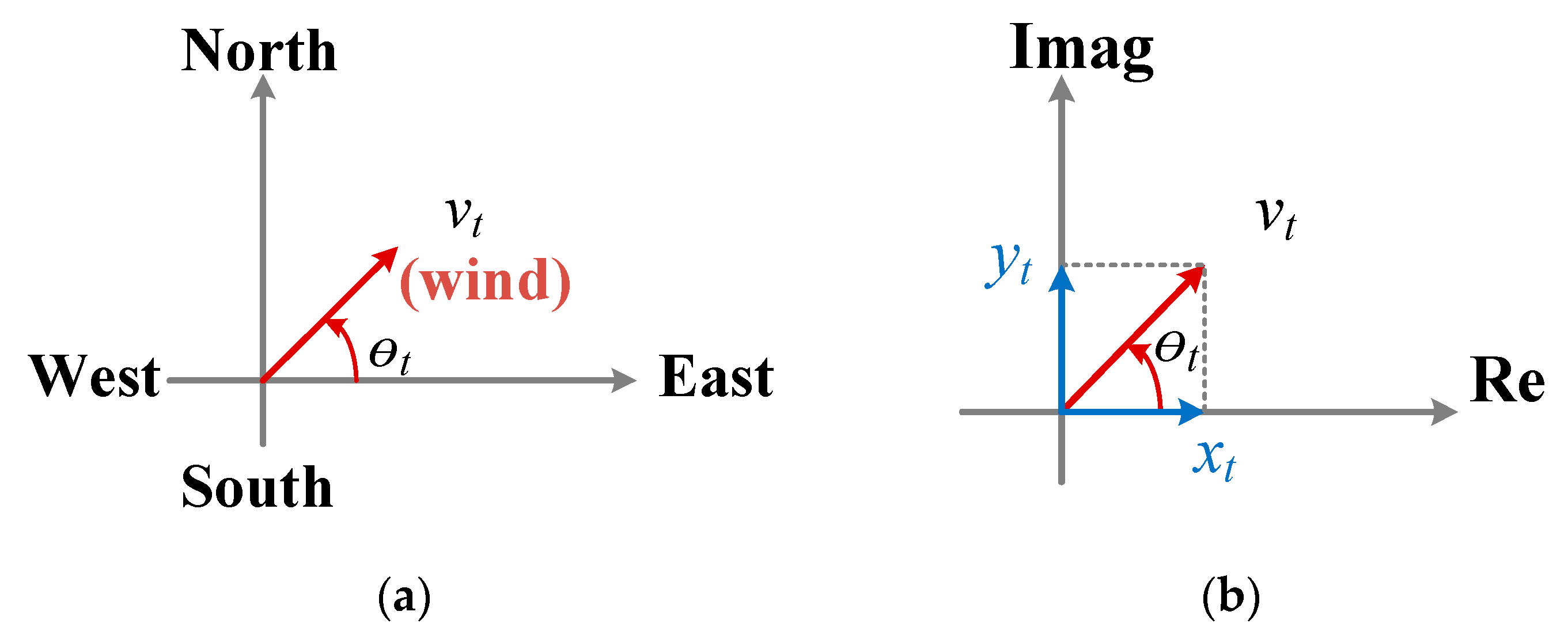
2.1. Wind Vector
At time
, the wind is characterized by its speed
and direction
[
18]. The wind can be represented in its vector form as shown in
Figure 1a. The wind vector has two components,
along the real axis and
along the imaginary axis as shown in
Figure 1b. The
wind is parallel to the
axis. To be more specific, a positive or negative
represents wind blowing from the west or east, respectively. On the other hand, the
wind runs parallel to the
axis. More specifically, a positive or negative
represents wind blowing from the south or north, respectively.
Several meteorological parameters are considered for improving the performance of the wind forecast. The methods in [
19,
20,
21,
22] propose the use of wind direction along with wind speed to reduce forecasting error. Methods using the wind vector applying both the speed and direction of the wind are available in [
18,
23]. The method in [
23] uses a complex-evaluated neural network (CVNN) for the prediction of the performance of a wind power generation station. The inputs for the CVNN are complex numbers representing the wind speed and direction. Simulation tests are performed to demonstrate the efficacy of the proposed prediction method.
This paper uses the complex components of the wind vector and as the input parameters for the ANN-based forecasting models. The components of the wind vector and are reconstructed from the estimated values of the and using Equations (1) and (2).
2.2. Interpolation Methods
Interpolation [
24] is a numerical, analysis-based technique for estimating values within the range of a specified discrete set of data points. Given a set of data points in a plane between the bounding interval [
a,
b], an interpolating function can be used to estimate a missing data point in the interval. Consider a set of
data points on the curve of an unknown function
defined as {
,
,
,
}. The objective is to identify an interpolation function
fi(
x) that approximates the function
in the interval
. In this case,
and
.
The interpolation techniques can be classified into two categories [
25]. The first category is referred to as the global interpolation, where a single high-degree polynomial function is determined to match all the available data points. Though this technique provides a smooth curve, there is a possibility of extreme oscillations. Most engineering applications and processes do not possess such high-degree polynomial functions. The second category is the piece-wise interpolation, where multiple low-degree polynomial functions are determined for smaller intervals. In this context, an interpolant function estimates the values of another function over a smaller interval. Therefore, a set of interpolant functions may be used for successive data intervals.
This paper examines six different interpolation techniques to obtain perturbed observations from the original dataset. A brief overview of these methods is provided in the following subsections.
2.2.1. Next-Neighbor Interpolation
The next-neighbor interpolation assumes the missing value to be the same as the next available data value. For example, consider two consecutive known data points: () and (). The next-neighbor interpolation estimates the value of any unknown data points in the range as .
2.2.2. Previous-Neighbor Interpolation
The previous-neighbor interpolation operates similarly to the next-neighbor interpolation. The only difference is that the unknown values in the range are estimated as .
2.2.3. Linear Interpolation
The linear interpolation assumes that any two consecutive known data points are connected by a straight line. Using the example from
Section 2.2.1, the linear interpolation over the range
is governed by:
where the slope of the line
is calculated as:
and the constant
can be obtained using Equations (3) and (4) as:
The advantage of using linear interpolation is its simplicity and low computational complexity in reconstructing a signal [
26].
2.2.4. Cubic Interpolation
The cubic interpolation assumes the function
as a cubic polynomial. For the range
, the interpolant function is represented as follows:
The unknown coefficients
,
,
, and
can be determined using two different methods namely, the cubic spline and the Piecewise Cubic Hermite Interpolating Polynomial (PCHIP). Both of these interpolation techniques are discussed next.
Cubic Spline: This is one of the most commonly used piecewise interpolation techniques. For data points (
) where
and
, the cubic spline interpolation requires to obtain a solution function
[
27]:
where each
is a continuous polynomial of order
3. In a generic form:
To determine
, we need the coefficients
,
,
, and
for each
. For
intervals, there are
coefficients to be determined and therefore
equations are needed. For any successive data points, the spline requires,
and
Rewriting Equations (9) and (10) in the form of Equation (8),
and
Applying Equations (11) and (12) to each
, we can obtain 2
equations. As discussed in [
27], the function
is smooth and has continuous derivatives
and
in the range
. To have a smooth function, at each of the points
,
,
,
,
From Equation (8) we obtain,
and
Rewriting Equations (13) and (14) using Equations (15) and (16), we have,
and
When applied to all points
,
,
,
, Equations (11) and (12) result in
equations. So far, we have
equations and need two more equations. Therefore, the boundary condition:
is applied to obtain two more equations [
27]. Now, we have
linear equations to be solved for obtaining the
coefficients in
. These equations can be solved using any linear equation solver.
PCHIP: This is another form of piecewise cubic interpolation. The PCHIP uses different conditions to estimate the slope of the cubic polynomial and calculate the coefficients of the polynomial [
28]. Interpolation using the PCHIP method preserves the monotony, positivity, and convexity of the data [
29]. The polynomial
resulting from the PCHIP has the following properties:
- 1.
For each subinterval , the polynomial is a cubic Hermite polynomial with defined derivatives at each data point.
- 2.
The first derivative is continuous, while the second derivative may or may not be continuous.
- 3.
The PCHIP is shape-preserving. This means that the slopes at each data point are chosen to preserve the shape of the data. Therefore, the data interval where the data is monotonous so is . At a local extremum of the data, also has a local extremum.
For each interval
, the interpolant function
is defined as:
where:
and the
, for
, are the cubic Hermite basis functions defined as,
where:
The three-point difference formula [
30] can be used to compute
in Equation (21). Then, using Equation (21) through (28) the function
can be constructed.
2.2.5. Fast Fourier Transform (FFT)
FFT can be used to convert discrete time-domain data into the frequency domain, and vice-versa. As to this interpolation technique, the discrete data set
sampled at a constant frequency
is first transformed to the frequency domain using:
represents the
th frequency component of the signal. The interpolant function can be obtained using the inverse transform as follows,
Thus, applying Equations (29) and (30) to the interpolant function can be constructed and used to obtain the perturbed values.
2.3. Ensemble Forecasting and Perturbed Observations
The concept of ensemble model is based on using the output of multiple members in the network in order to come up with an aggregated decision. This aggregated decision is expected to outperform a single-prediction method.
The ensemble model was first discussed in the context of weather forecasting by Galmarini et al. [
9]. In their work, the authors have proved that using the ensemble model can actually improve accuracy of forecasting prediction.
On the other hand, perturbed observation is a technique used to generate several distinguishable observations out of the original one. Generating multiple observation can help in overcoming uncertainties in the model. As a result, introducing perturbed observations can help in reducing the errors in prediction, which will ultimately improve the overall accuracy of prediction.
Perturbed observations ensemble models generate an ensemble of parallel forecasts for each data cycle, and the networks will differ from each other by having different input data. In each data cycle, a set of unique observations of multi-step-ahead predictions will be received from each model that is used in the ensemble network model. These observations are called ensemble members, which are used to calculate the final forecasted value in deterministic or probabilistic nowcasting forms.
3. Prediction Model
This work proposes a new model for the nowcasting of wind speed and direction using ensemble neural networks. The accuracy of ensemble neural networks can be improved using perturbed observations generated using data splitting and interpolation techniques. This has been demonstrated for the prediction of the short-term wind forecast in [
4]. The proposed model consists of four stages, as represented in
Figure 2. These stages are discussed in the following subsections.
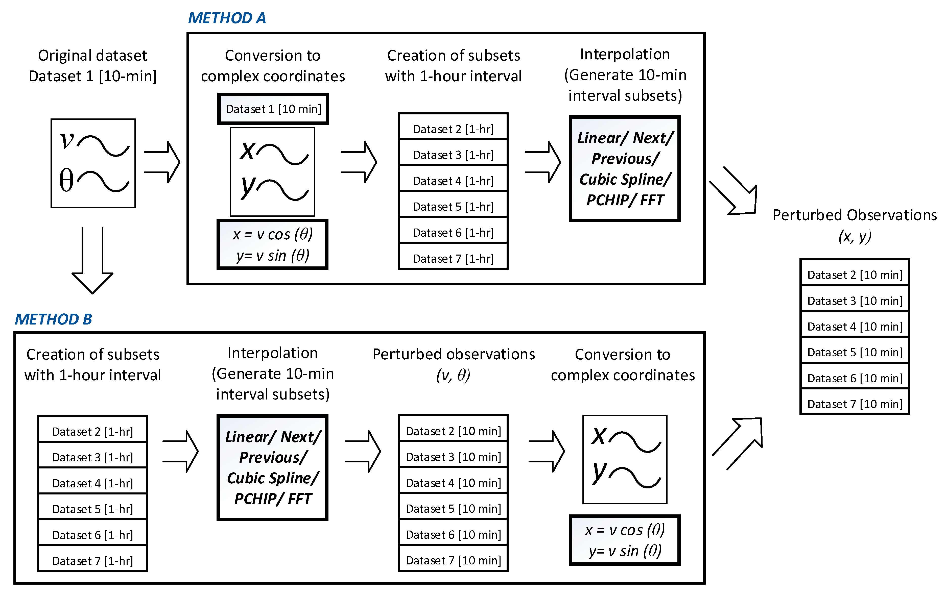
3.1. Pre-Processing
This stage processes the available 10 min interval wind speed dataset ‘Dataset 1′ and generates the perturbed observations using the selected data splitting and interpolation techniques. Two different methods can be used to obtain the perturbed observations:
The steps involved in this method are as follows:
- 1.
The wind speed and its direction are first transformed into their complex plane coordinates .
- 2.
Six different 1 h interval subsets are created from the complex representation of the original dataset ‘Dataset 1′ using the data splitting technique.
- 3.
For each subset, a new dataset of 10 min intervals is created using one of the interpolation techniques.
As to this method, the original dataset is first interpolated to form perturbed observations and then converted to complex plane coordinates. The steps involved in this method are as follows:
- 1.
Six new 1 h interval subsets containing the wind speed and its direction are created from the original dataset ‘Dataset 1′ using data splitting techniques.
- 2.
For each dataset, the chosen interpolation technique is applied to obtain new subsets with 10 min intervals.
- 3.
Each of the new datasets is converted to its complex coordinate form, i.e., .
A diagrammatic representation of both these methods is shown in
Figure 3. The output datasets from this stage are forwarded as input to the next stage.
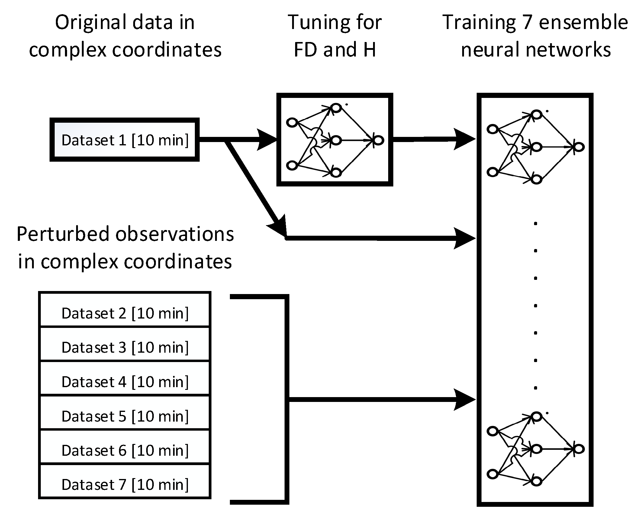
3.2. ANN Training
The input/feedback delay (
) ratio and the number of hidden layer neurons (
) need to be fixed to train the neural network model. This stage first tunes a single neural network to obtain ideal
and
H values using the original data (Dataset 1). With these tuned parameters, seven ensemble neural networks are created and trained using the seven available datasets (i.e., one original and six perturbed observations). A flow diagram for stage 2 is shown in
Figure 4. This ensemble of trained neural networks is used in the following stage to perform nowcasting.
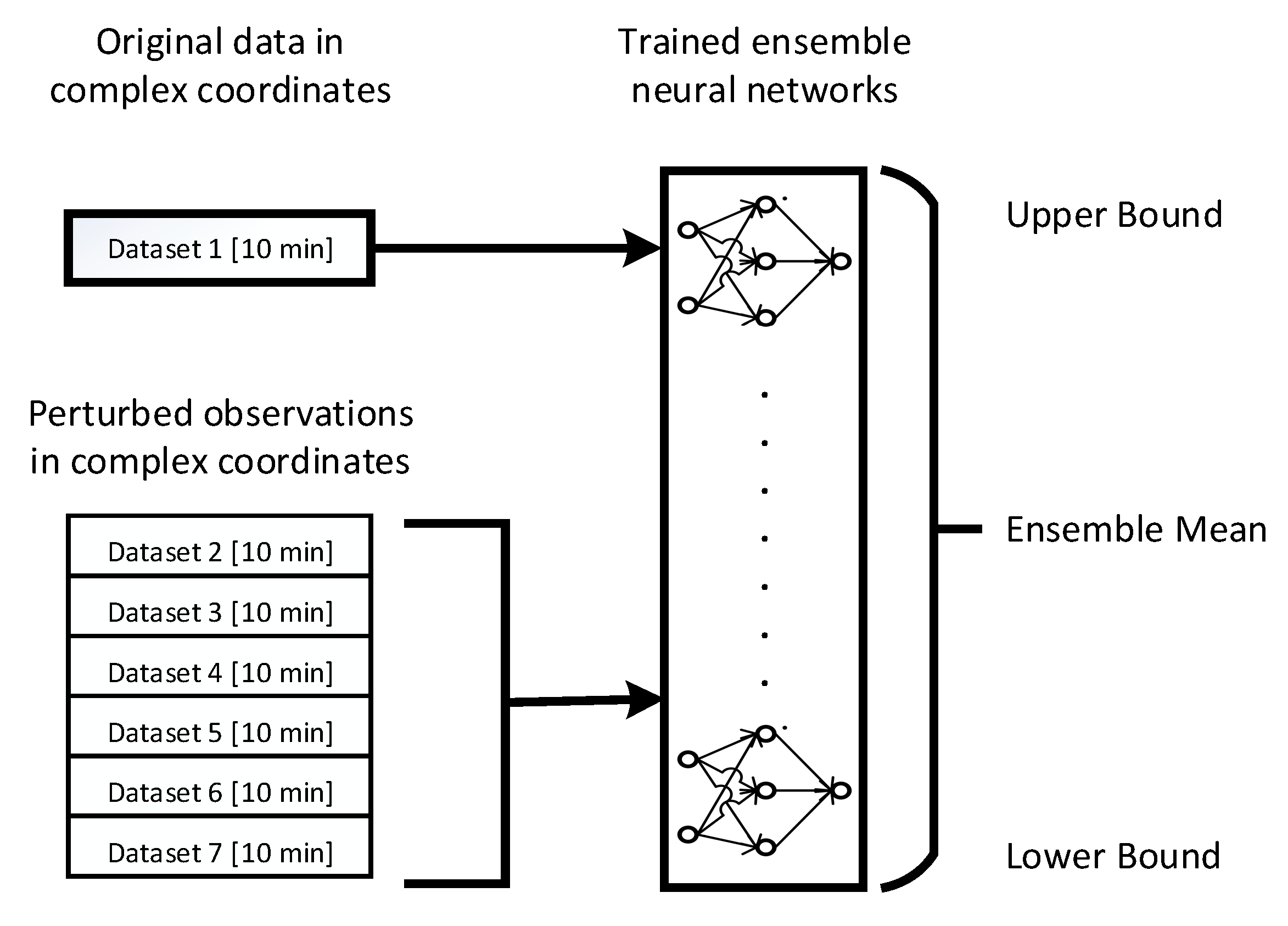
3.3. Nowcasting
This stage uses the seven trained ensemble neural networks to perform multi-step nowcasting of wind speed and direction. Similar to the training stage, this stage uses the seven available datasets for prediction as shown in
Figure 5. The model provides a mean value for the forecast along with the upper and lower bounds for probabilistic estimations.
3.4. Post-Processing
The post-processing stage processes the predicted wind speed and direction from the nowcast stage to obtain the wind turbine output estimates. The reader is reminded that the output scales of the nowcasting stage are in the complex coordinate form.
This stage consists of three steps, which are detailed below.
- 1.
The nowcasting output scales are converted to the original wind vector component form using Equations (1) and (2).
- 2.
The mean, standard deviation, and upper and lower bounds of the scales from step 1 are calculated to obtain the deterministic and probabilistic estimates for
and
as in [
4]. To evaluate the performance of the prediction method, the mean square error (
MSE), normalized root-mean-square error (
nRMSE), correlation coefficient (
R), prediction interval coverage probability (
PICP), and prediction interval nominal average width (
PINAW) are calculated using Equations (31)–(35):
where
and
are the actual observation (target value) and the deterministic output of the
th predicted sample, respectively. Additionally,
is the number of predicted samples.
where
is the range of the target observations.
where the coverage coefficient (
) equals 1 if the actual observation
falls within the prediction interval (
) with lower bound
and upper bound
, and 0 otherwise. This can be represented as:
Most of the prior literature for the prediction of wind speed and direction provides only the
PICP value for the proposed models and not the
PINAW values. Unlike
PICP, the
PINAW value can be used to determine the accuracy of the predicted values. Therefore, this paper provides the
PINAW values as well:
- 3.
The nowcasting of the wind data is used to estimate the output of the wind turbine. For the prediction of wind speed data, the model of the ‘Dhofar Wind project′ at Harweel, Sultanate of Oman is used as demonstrated by the authors in [
5].
4. Simulation Setup
This paper uses a dataset of measured parameters from the “Dhofar Wind Project” in Harweel, Sultanate of Oman. The dataset includes several parameters such as wind speed and direction, temperature, humidity, and pressure. Those measurements were recorded at different altitudes during the period from November 2013 to October 2015. The average wind speed measurements were obtained at an altitude of 79 m, while temperature and pressure measurements were obtained at an altitude of 76 m. A more detailed description of this dataset is available in [
4].
The wind speed measurements were used to train the ensemble neural networks formed using FFTDNN, NAR, and NARX. However, given that NARX accepts exogenous inputs, other parameters can be used with this type of neural network. Specifically, temperature and pressure were used along with time, date (i.e., day and month), seasons viz. winter (January–February), spring (March–May), summer (June–August), and autumn (September–October).
As discussed earlier, there are several types and structures of neural networks that can be used to predict wind speed and direction. Each of these networks can be trained using a variety of algorithms. Furthermore, the data used in training those neural networks can be pre-processed through multiple techniques (i.e., different data splitting, interpolation, etc.). The mix-and-match of these network types, structures, training algorithms, and data pre-processing techniques would result in numerous combinations. Each of these combinations may excel in one aspect but fall short in others.
Therefore, one of the objectives of this work is to exhaustively explore these combinations in terms of prediction accuracy and execution time. This design space exploration is very useful for the following reasons; (1) it allows the researcher to find the most optimal combination that would yield the highest prediction rate for wind speed and direction, (2) it provides a means of understanding the dynamics that the network type, training algorithm, and pre-processing technique play in terms of prediction accuracy and execution speed, (3) it allows researchers to perform tradeoffs between prediction accuracy and execution time by knowing how each of these combinations performs, and (4) this design space exploration provides researchers with a list of favorable configuration candidates that can be used for wind speed and direction prediction; regardless of the dataset used. The rest of this section discusses the process that was followed to generate these combinations.
An initial nowcasting network model is trained using FFTDNN, NAR, and NARX models. As for NARX neural network, three models are considered by changing the exogenous inputs. In particular, the first NARX model (NARX1) accepts three inputs; namely, time, date, and season. The second NARX model (NARX2) accepts two inputs only; namely, temperature and pressure. The third NARX model (NARX3) accepts five inputs; namely: time, date, season, temperature, and pressure. This results in a total of five neural network models (i.e., FFTDNN, NAR, and three NARX models with different exogenous inputs).
Four features were used to tune the ensemble neural network discussed above. These are detailed below:
Feature 1: Four different training algorithms were used; namely, Levenberg-Marquardt backpropagation (LM), Bayesian Regularization backpropagation (BR), Scaled Conjugate Gradient backpropagation (SCG), and Resilient backpropagation (RP).
With regards to Features 3 & 4, we consider a specific range for FD and . The main reason for this selection is to control the size of the design space. Additionally, there is a tradeoff between number of nodes and the cost of the design in terms of execution time and processor load.
The mix-and-match of the above features results in numerous combinations. Each combination is used to tune a single ANN network (i.e., a single configuration). Based on preliminary simulation results, the top eight configurations that yield the best tuning for each network type were chosen; resulting in 40 different configurations as shown in
Table 1. The column labeled ‘Abbreviation′ in the table indicates how the ANN network was tuned. The column uses the notation N-T-D, where:
‘N′ is the type of neural network: FFTDNN, NAR, or NARX,
‘T′ is the training algorithm, which is one of the algorithms specified in ‘Feature 1′ above, and
‘D′ is the splitting technique, which is one of the two methods specified in ‘Feature 2′ above.
Computer simulations were carried out to assess the performance of the 40 model configurations presented in
Table 1. The results of the simulations are discussed in detail in the following section.
5. Results and Discussions
To expand the design space exploration of the proposed prediction model, each neural network configuration provided in
Table 1 is simulated using different variations within the pre-processing stage shown in
Figure 2. In particular, the two methods discussed in
Section 3.1 were considered as two different means of generating perturbed observations. Furthermore, we have experimented with the six interpolation techniques presented in
Section 2.2. Therefore, we have a total of 40 × 2 × 6 = 480 models for the comparative study. Given that we are including additional variations, we should update the notation presented in the Abbreviation column of
Table 1. As such, we shall use henceforth the notation N_T_D_I_M, where ‘N′ is the type of the neural network, ‘T′ is the training algorithm, ‘D′ is the splitting technique, ‘I′ is the interpolation technique, and ‘M′ is the method used to generate perturbed observations.
The performance of each of the 480 models is evaluated using
MSE,
nRMSE,
R,
PICP,
PINAW metrics (see
Section 3.4). A better-performing model is characterized by a lower
MSE,
nRMSE, and
PINAW and a higher
R and
PICP.
While prediction accuracy is a very important metric in assessing the performance of a neural network, however, the execution time of a model is as important. This is especially true for applications that require fast prediction of wind speed and direction. Therefore, the execution time is measured to determine their practicality when used in such applications.
Moreover, a Wake model was used to estimate the generated power from the wind farm at the “Dhofar Wind project” using the predicted wind speed and direction [
4]. A comparative analysis is conducted between the estimated and actual power output from the wind farm.
5.1. Prediction Performance
Several MATLAB simulations were performed on the 480 variations of the prediction model. Based on the results of these preliminary simulations, we present here the 18 best-performing variations.
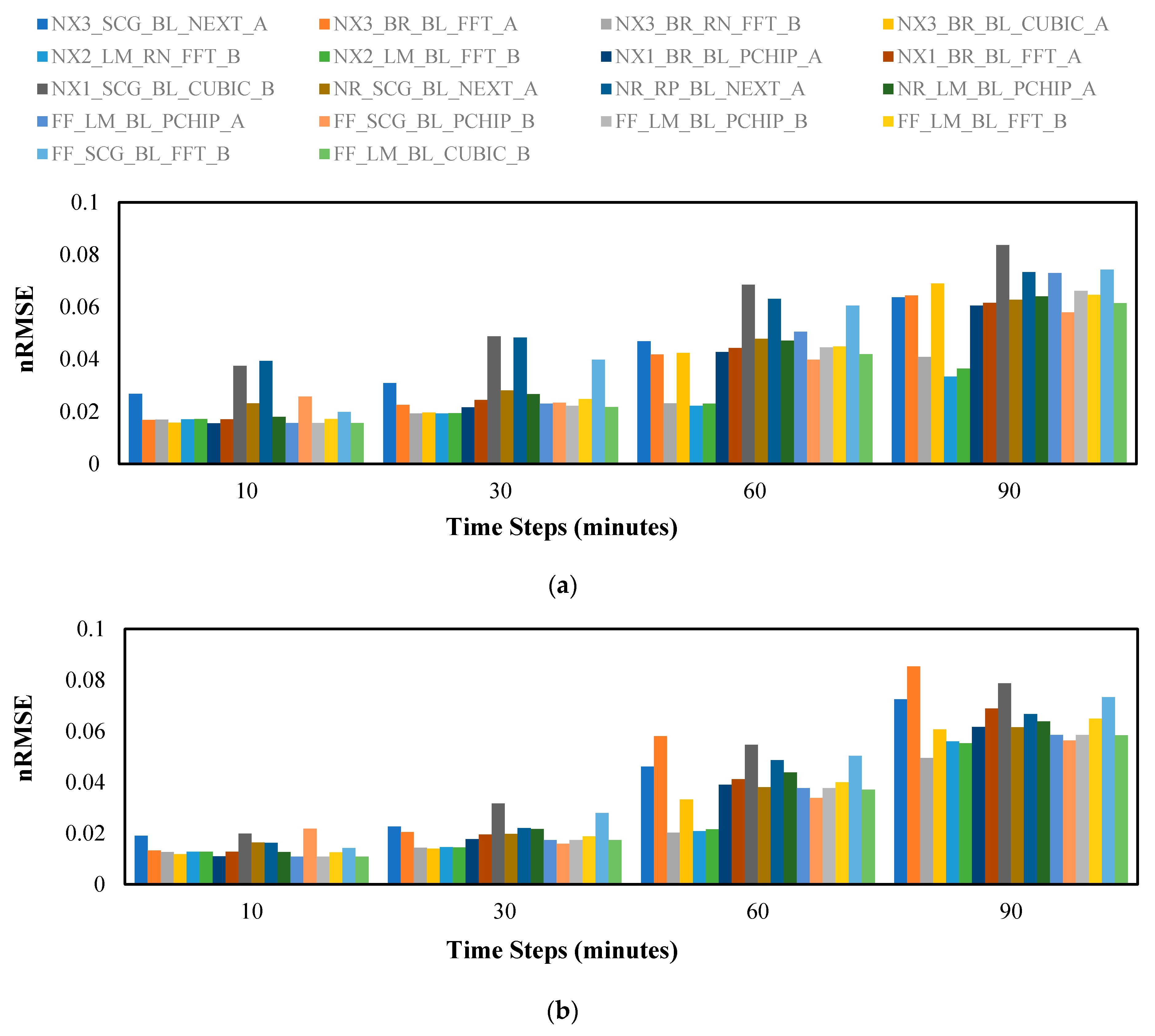
Figure 6 shows the performance in terms of
nRMSE for both wind speed and direction predictions, which was calculated using Equation (32). As mentioned earlier, a lower
nRMSE value implies better prediction accuracy. Therefore, as the time horizon of the forecast increases, the
nRMSE value of the variations deteriorates.
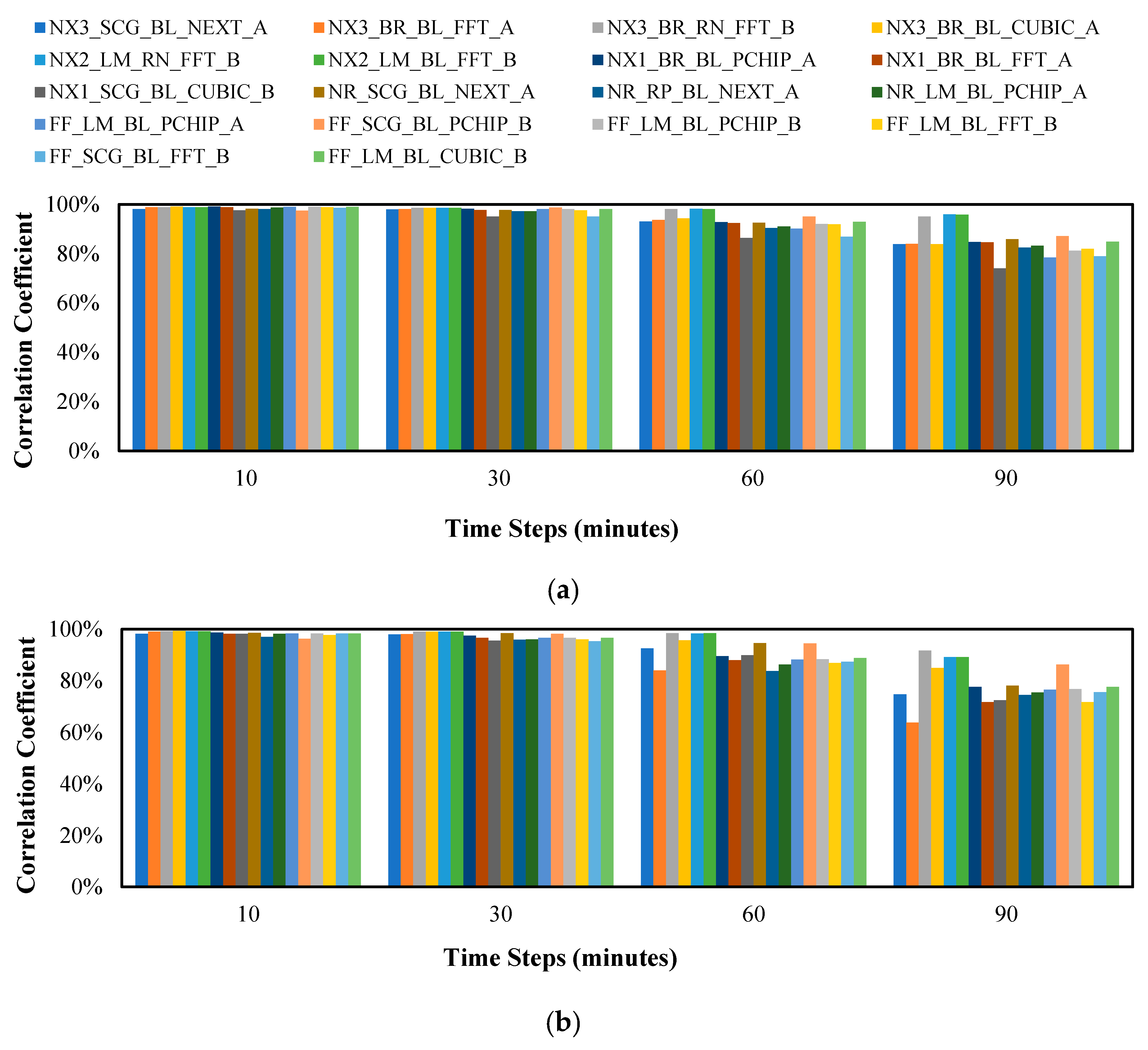
The performance of the variations in terms of the correlation coefficient (
), which was calculated using Equation (33) is shown in
Figure 7. The figure shows that as the prediction steps increases (i.e., nowcasting further in time) the prediction accuracy decreases.
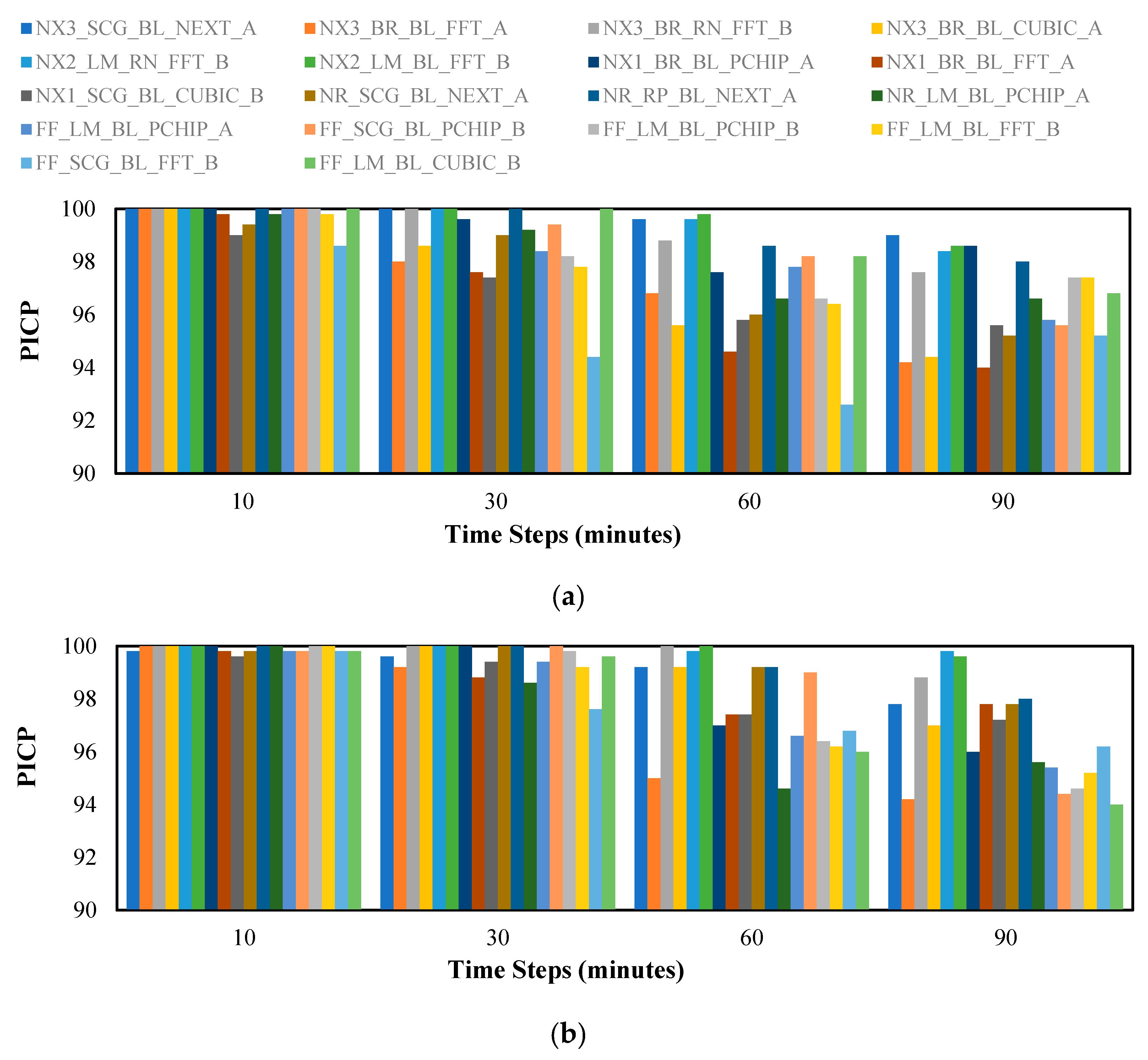
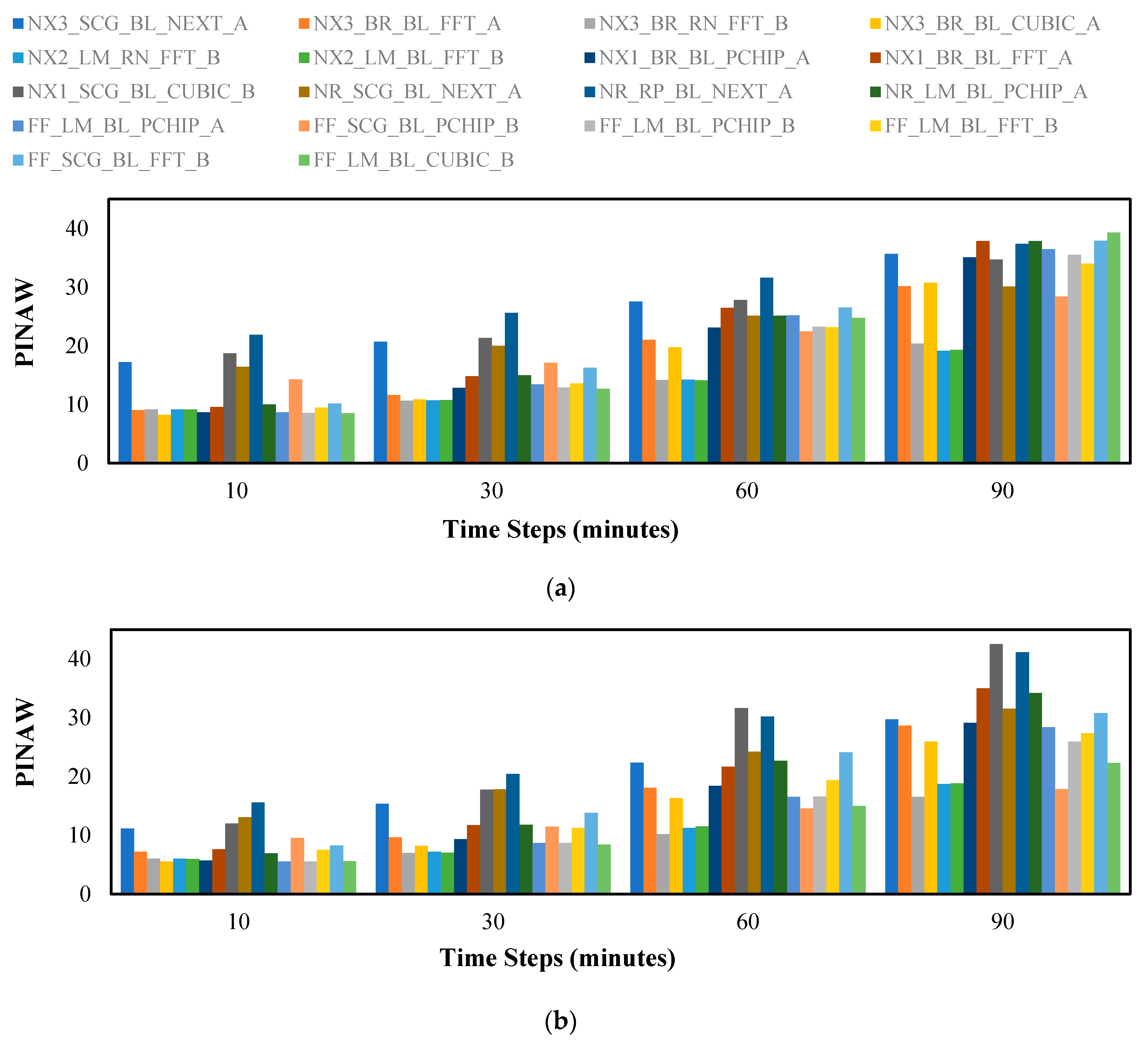
Figure 8 and
Figure 9 show the prediction performance in terms of
PICP and
PINAW as calculated using Equations (34) and (35), respectively.
The plots shown in
Figure 6 to
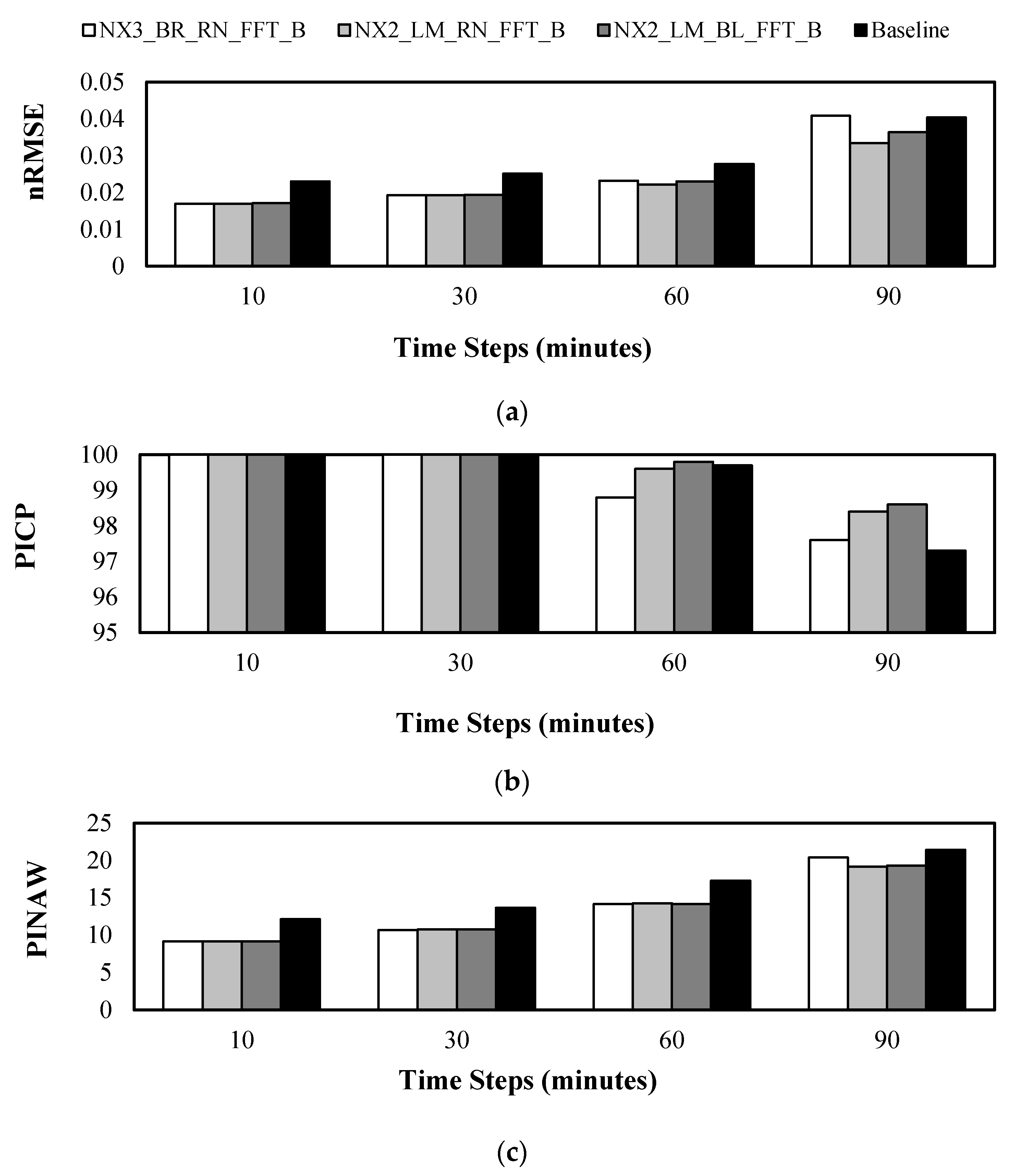
Figure 9 were studied extensively and the variations were compared to one another thoroughly. Based on these comparisons, we find that the 3 top models that perform well in predicting both speed and direction are: (1)
NX3_BR_RN_FFT_B, (2)
NX2_LM_RN_FFT_B, and (3)
NX2_LM_BL_FFT_B. Interestingly, the model
NX2_LM_BL_FFT_B has outperformed the other two contenders, especially in the
PICP metric for the 60 min and 90 min prediction. An observation worth mentioning here is that the NARX structure outperforms the two other neural network types. In addition, the use of FFT interpolation complemented with Method B of generating perturbed observations results in better prediction performance.
Next, we compare the wind speed prediction performance of the 3 top models to the NARX model described in [
4] as illustrated in
Figure 10. In terms of
nRMSE,
Figure 10a, the proposed models
NX3_BR_RN_FFT_B,
NX2_LM_RN_FFT_B, and
NX2_LM_BL_FFT_B show 26.29%, 26.16%, and 25.65% improvement over the model in [
4] for the 10 min-ahead nowcast, respectively. Similarly, for the 60 min-ahead nowcast, we observe an improvement of 16.44%, 20.14%, and 17.09%, respectively. As for the 90 min-ahead speed nowcast, both
NX2_LM_RN_FFT_B and
NX2_LM_BL_FFT_B outperformed the NARX model.
The comparison of
PICP,
Figure 10b, shows that there is no significant improvement in the 10 and 30 min time steps. However, as the time steps increase, the performance gain becomes more visible. For example, in the 90 min-ahead nowcast, the three models:
NX3_BR_RN_FFT_B,
NX2_LM_RN_FFT_B, and
NX2_LM_BL_FFT_B show a
PICP improvement of 0.30%, 1.13%, and 1.34%, respectively.
As for the
PINAW metric,
Figure 10c, a noticeable improvement is observed across all time steps. For example, at 90 min-ahead nowcast,
NX2_LM_BL_FFT_B shows an improvement of 9.88% compared to the baseline.
The proposed models outperform the baseline in all metrics. It should be noted here that we are unable to compare the wind direction prediction rate of the proposed models to the baseline since the latter did not perform such prediction.
5.2. Execution Time
The execution time for the three best-performing models was measured using a computer with an Intel 4th Generation Core i5 processor and 8 GB DDR RAM. All the three models have an execution time of less than 0.7 s for nowcasting one sample (See
Table 2). In particular, the
NX2_LM_BL_FFT_B model was the fastest among the three models, which could be attributed to a structure that has lesser exogenous inputs and a lower number of neurons.
5.3. Estimation of Generated Power
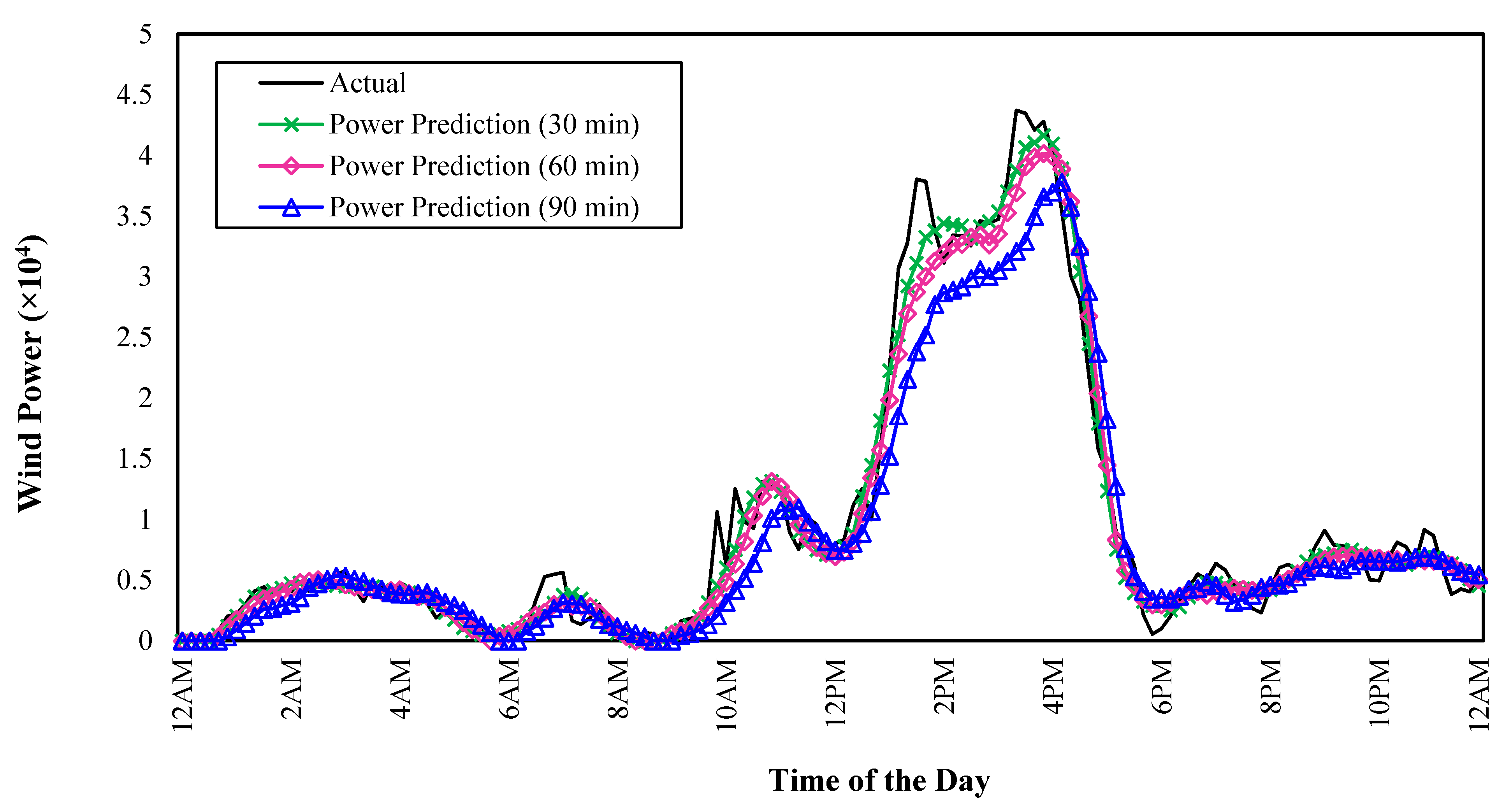
The power utilities use an energy management system (EMS) for power system planning and operation. Due to the intermittency associated with the wind, the EMS requires an accurate forecast for the power generation from wind farms to avoid any high-power ramp events. The proposed wind speed and direction prediction model can be incorporated in an EMS to predict the power generated by the wind farms. To understand the reliability of the proposed model when used in an EMS, the predicted wind speed and direction are used to estimate the power output from the 32.5MW “Dhofar Wind Project”. Similar to [
2], the three-dimensional multi-speed and direction Wake model is used for generating the power estimate from the wind farm. However, unlike the previous work, we use both the wind speed and direction for estimating the power output from the wind farm. The study is performed using actual weather and power data recorded at the “Dhofar Wind Project” on a winter day. The deterministic power output estimated using the wind speed and direction predicted using the
NX2_LM_BL_FFT_B model is compared with the actual measurements as shown in
Figure 11. A high correlation of 98.71%, 98.41%, and 96.79% is observed for the 30 min, 60 min, and 90 min ahead nowcasts, respectively.
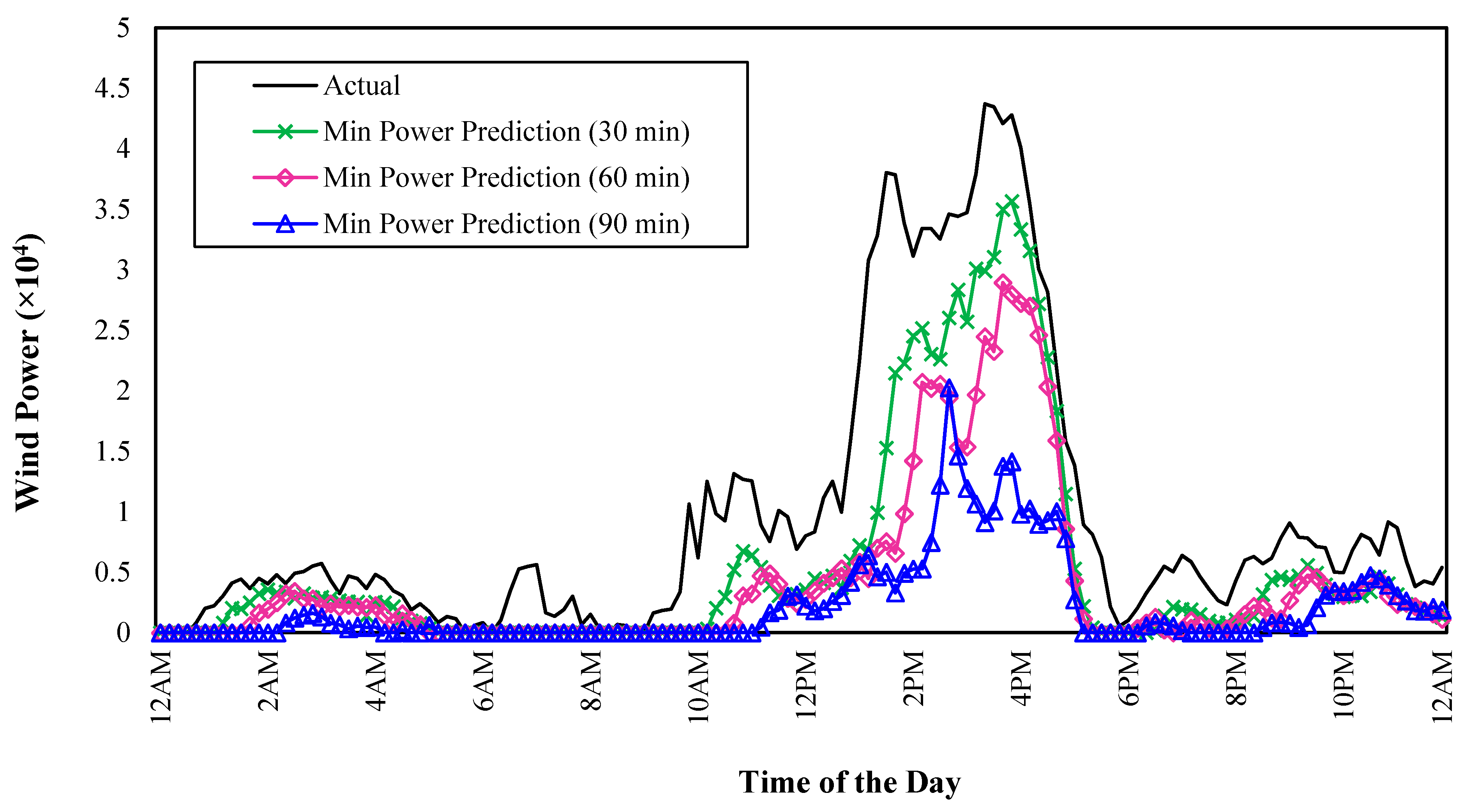
In addition to the 30 min-ahead nowcast for the power output, the predicted minimum power output—calculated with 95% confidence—for 30 min, 60 min, and 90 min ahead nowcasts are compared with the measured power generation (See
Figure 12). Such accurate power generation estimates will assist the EMS in taking critical power dispatch decisions. Using the minimum power production estimates for the 30 min, 60 min, and 90 min ahead scenarios, a dispatch level can be decided to avoid any undue power system risks.
In order to show the overall improvement in prediction accuracy,
Table 3 demonstrates a comparison between the three selected models with the baseline [
4]. The table clearly shows that incorporating the wind direction has improved the estimation of the generated power. In fact, the larger the time horizon, the more benefits can be gained from including the wind direction as an input to the predictor.
6. Conclusions and Future Work
This paper proposed a model for nowcasting wind speed and direction. The model involves several novelties in its approach. First, the model employs several interpolation techniques in order to generate perturbed observations. The latter are used to mitigate any potential uncertainties while training the ensemble neural networks. The trained ensemble neural networks are then used to nowcast wind speed and direction.
Additionally, the paper presented an exhaustive investigation that consisted of tens of different configurations that were explored to find the best combination of neural network type, training algorithm, interpolation techniques, and data splitting techniques. The proposed prediction models not only can predict both speed and direction but also show improved prediction rates over other contenders.
For the proposed model, 480 different configurations were generated. Those configurations constitute various neural network types and techniques for training, data splitting, interpolation, and perturbed observations. Those configurations were simulated to evaluate their performance. The paper utilized several metrics to assess the performance of these configurations. These metrics include nRMSE, PICP, PINAW, and correlation coefficient. Based on the result, the three best models were selected for further investigation. In fact, these models were found to outperform a baseline model in terms of accuracy and execution time.
The simulation results show that NARX-based neural networks outperform other networks that utilize NAR and FFTDNN. In addition, we observe that models that use FFT interpolation technique for the perturbed observations generation exhibit an improved prediction accuracy for both wind speed and direction. More specifically, the simulation results show that the configuration NX2_ML_BL_FFT_B has scored an nRMSE as low as 0.036 for 90 min ahead prediction. The same configuration has outperformed other contenders in terms of PICP by scoring 98.6.
Furthermore, the paper assessed the execution time of the models. This is important given that frequent and rapid updates to the prediction help the operators to prepare an adequate dispatch plan. We find that the three best models maintain a rapid execution time of 0.7 s per sample.
Finally, the paper estimates the power generated from an actual wind farm based on the nowcasting performed on the wind speed and direction. It was observed that the estimated power using the proposed model is very close to the actual measured values. More specifically, the simulations show a high correlation of 98.71%, 98.41%, and 96.79% for the 30 min, 60 min, and 90 min ahead nowcasts, respectively.
For future extension of this work, comparative experiments with different wind farm datasets may be performed.
Author Contributions
Conceptualization, S.A.-Z., A.A.M., A.A.-H. and S.A.Y.; methodology, S.A.-Z. and A.A.M.; software, S.A.-Z. and M.B.; validation, S.A.-Z.; data curation, S.A.-Z., A.A.M. and S.A.Y.; writing—original draft preparation, S.A.-Z., A.A.M. and S.G.; writing—review and editing, A.A.M., S.G. and R.A.A.; supervision, A.A.M., A.A.-H., and R.A.A.; project administration, A.A.-H.; funding acquisition, A.A.-H. All authors have read and agreed to the published version of the manuscript.
Funding
This research was funded by His Majesty Trust Fund (SR/ENG/ECED/17/01) and the Ministry of Higher Education, Research, and Innovation Fund (RC/RG-ENG/ECED/19/03). The APC was funded by the same grants.
Acknowledgment
The authors would like to express their thanks and deep appreciation to the Directorate General of Meteorology, Civil Aviation Authority for providing the meteorological data used in this study.
Institutional Review Board Statement
Not applicable.
Informed Consent Statement
Not applicable.
Conflicts of Interest
The authors declare no conflict of interest. The funders had no role in the design of the study; in the collection, analyses, or interpretation of data; in the writing of the manuscript, or in the decision to publish the results.
References
- Wendorf, M. Settling the Debate: What Really Caused the Texas Electricity Blackout? Interesting Engineering. 2021. Available online: https://interestingengineering.com/what-caused-the-texas-electricity-blackout (accessed on 27 May 2021).
- Abdel-Karim, N.; Lauby, M.; Moura, J.N.; Coleman, T. Operational Risk Impact of Flexibility Requirements and Ramp Forecast on the North American Bulk Power System. In Proceedings of the 2018 IEEE International Conference on Probabilistic Methods Applied to Power Systems (PMAPS), Boise, ID, USA, 24–28 June 2018; pp. 1–6. [Google Scholar] [CrossRef]
- Zhang, J.; Cui, M.; Hodge, B.-M.; Florita, A.; Freedman, J. Ramp forecasting performance from improved short-term wind power forecasting over multiple spatial and temporal scales. Energy 2017, 122, 528–541. [Google Scholar] [CrossRef]
- Al-Zadjali, S.; Al Maashri, A.; Al-Hinai, A.; Al-Yahyai, S.; Bakhtvar, M. An accurate, light-weight wind speed predictor for renewable energy management systems. Energies 2019, 12, 4355. [Google Scholar] [CrossRef]
- Kirbas, I.; Kerem, A. Short-Term Wind Speed Prediction Based on Artificial Neural Network Models. Meas. Control 2016, 49, 183–190. [Google Scholar] [CrossRef]
- Ramasamy, P.; Chandel, S.S.; Yadav, A.K. Wind speed prediction in the mountainous region of India using an artificial neural network model. Renew. Energy 2015, 80, 338–347. [Google Scholar] [CrossRef]
- Senthil Kumar, P.; Lopez, D. Forecasting of wind speed using feature selection and neural networks. Int. J. Renew. Energy Res. 2016, 6, 833–837. [Google Scholar]
- Fazelpour, F.; Tarashkar, N.; Rosen, M.A. Short-term wind speed forecasting using artificial neural networks for Tehran, Iran. Int. J. Energy Environ. Eng. 2016, 7, 377–390. [Google Scholar] [CrossRef]
- Galmarini, S.; Bianconi, R.; Bellasio, R.; Graziani, G. Forecasting the consequences of accidental releases of radionuclides in the atmosphere from ensemble dispersion modelling. J. Environ. Radioact. 2001, 57, 203–219. [Google Scholar] [CrossRef]
- Do, L.N.N.; Taherifar, N.; Vu, H.L. Survey of neural network-based models for short-term traffic state prediction. Wiley Interdiscip. Rev. Data Min. Knowl. Discov. 2019, 9, 1285. [Google Scholar] [CrossRef]
- Jha, G.K.; Sinha, K. Time-delay neural networks for time series prediction: An application to the monthly wholesale price of oilseeds in India. Neural Comput. Appl. 2014, 24, 563–571. [Google Scholar] [CrossRef]
- Di Piazza, A.; Di Piazza, M.C.; Vitale, G. Estimation and forecast of wind power generation by FTDNN and NARX-net based models for energy management purpose in smart grids. Renew. Energy Power Qual. J. 2014, 1, 995–1000. [Google Scholar] [CrossRef]
- Ibrahim, M.; Jemei, S.; Wimmer, G.; Hissel, D. Nonlinear autoregressive neural network in an energy management strategy for battery/ultra-capacitor hybrid electrical vehicles. Electr. Power Syst. Res. 2016, 136, 262–269. [Google Scholar] [CrossRef]
- Sohoni, V.; Gupta, S.C.; Nema, R.K. A Critical Review on Wind Turbine Power Curve Modelling Techniques and Their Applications in Wind Based Energy Systems. J. Energy 2016, 2016, 8519785. [Google Scholar] [CrossRef]
- IEA. CO2 Emissions from Fuel Combustion—Highights. 2013. Available online: https://www.iea.org/reports/co2-emissions-from-fuel-combustion-overview (accessed on 26 May 2021).
- Hausfather, Z. Analysis: Global CO2 Emissions Set to Rise 2% in 2017 after Three-Year ‘Plateau’. Available online: https://www.carbonbrief.org/analysis-global-co2-emissions-set-to-rise-2-percent-in-2017-following-three-year-plateau (accessed on 20 November 2021).
- Coyle, E.D.; Simmons, R.A. Understanding the Global Energy Crisis; Purdue University Press: West Lafayette, IN, USA, 2014; Available online: https://www.jstor.org/stable/j.ctt6wq56p (accessed on 20 November 2021).
- Kitajima, T.; Yasuno, T. Output prediction of wind power generation system using complex-valued neural network. In Proceedings of the SICE Annual Conference, Taipei, Taiwan, 18–21 August 2010; pp. 3610–3613. [Google Scholar]
- Velázquez, S.; Carta, J.A.; Matías, J.M. Influence of the input layer signals of ANNs on wind power estimation for a target site: A case study. Renew. Sustain. Energy Rev. 2011, 15, 1556–1566. [Google Scholar] [CrossRef]
- Lange, M.; Heinemann, D. Relating the uncertainty of short-term wind speed predictions to meteorological situations with methods from synoptic climatology. In Proceedings of the European Wind Energy Conference, Madrid, Spain, 16–19 June 2003; p. 7. Available online: http://www.energymeteo.com/en/downloads/downloads.php (accessed on 21 May 2021).
- Tastu, J.; Pinson, P.; Kotwa, E.; Madsen, H.; Nielsen, H.A. Spatio-temporal analysis and modeling of short-term wind power forecast errors. Wind Energy 2011, 14, 43–60. [Google Scholar] [CrossRef]
- Gallego, C.; Pinson, P.; Madsen, H.; Costa, A.; Cuerva, A. Influence of local wind speed and direction on wind power dynamics—Application to offshore very short-term forecasting. Appl. Energy 2011, 88, 4087–4096. [Google Scholar] [CrossRef]
- Took, C.C.; Strbac, G.; Aihara, K.; Mandic, D.P. Quaternion-valued short-term joint forecasting of three-dimensional wind and atmospheric parameters. Renew. Energy 2011, 36, 1754–1760. [Google Scholar] [CrossRef]
- Phillips, G.M. Interpolation and Approximation by Polynomials; Springer: New York, NY, USA, 2003. [Google Scholar]
- Kaya, E. Spline Interpolation Techniques. J. Tech. Sci. Technol. 2014, 2, 47–52. [Google Scholar]
- De Boor, C. A Practical Guide to Splines; Mathematics of Computation; Springer: New York, NY, USA, 1978; Volume 27, Issue 149. [Google Scholar]
- Leal, L.A. Numerical Interpolation: Natural Cubic Spline. Towards Data Science. 2018. Available online: https://towardsdatascience.com/numerical-interpolation-natural-cubic-spline-52c1157b98ac (accessed on 27 May 2021).
- Rabbath, C.A.; Corriveau, D. A comparison of piecewise cubic Hermite interpolating polynomials, cubic splines and piecewise linear functions for the approximation of projectile aerodynamics. Def. Technol. 2019, 15, 741–757. [Google Scholar] [CrossRef]
- Abdul Karim, S.A.; Mohd Rosli, M.A.; Mohd Mustafa, M.I. Cubic spline interpolation for petroleum engineering data. Appl. Math. Sci. 2014, 8, 5083–5098. [Google Scholar] [CrossRef][Green Version]
- Akima, H. A New Method of Interpolation and Smooth Curve Fitting Based on Local Procedures. J. ACM 1970, 17, 589–602. [Google Scholar] [CrossRef]
Figure 1.
The representation of the wind speed and its direction (a) in Vector Form, and (b) in Complex Plane.
Figure 1.
The representation of the wind speed and its direction (a) in Vector Form, and (b) in Complex Plane.
Figure 2.
The process flow of the proposed prediction model.
Figure 2.
The process flow of the proposed prediction model.
Figure 3.
The two methods that can be used for pre-processing the dataset and generating the perturbed observations from the original dataset. Method A: the original dataset is converted to its complex format first and then the interpolation technique will be implemented. Method B: the interpolation technique is implemented first, and then the interpolated data sets are converted to the complex format.
Figure 4.
Training of the ensemble neural network model using seven datasets as input. The seven datasets include the original data set, and the remaining six are the output of previous stage of pre-processing
Section 3.1.
Figure 4.
Training of the ensemble neural network model using seven datasets as input. The seven datasets include the original data set, and the remaining six are the output of previous stage of pre-processing
Section 3.1.
Figure 5.
The Nowcasting Stage consists of seven trained ensemble neural networks capable of performing multi-step nowcasting of wind speed and direction. Nowcasting model is the same model used in previous stage of ANN training (
Section 3.2). The output will be used to get the estimated wind speed and its direction (the mean value of the multiple outputs), and the probabilistic estimation for the lower and upper bounds.
Figure 6.
The 18 best-performing variations in terms of nRMSE for (a) wind speed prediction, and (b) wind direction prediction. Note that 500 samples were used, each of which is a 10 min interval. This results in a total of ~83 h.
Figure 6.
The 18 best-performing variations in terms of nRMSE for (a) wind speed prediction, and (b) wind direction prediction. Note that 500 samples were used, each of which is a 10 min interval. This results in a total of ~83 h.
Figure 7.
The 18 best-performing variations in terms of the correlation coefficient (R) for (a) wind speed prediction, and (b) wind direction prediction, at different time horizon (i.e., 10, 30, 60, and 90 min). Note that 500 samples were used; each of which is a 10 min interval. This results in a total of ~83 h.
Figure 8.
The 18 best-performing variations in terms of PICP for (a) wind speed prediction, and (b) wind direction prediction, at different time horizon (i.e., 10, 30, 60, and 90 min). Note that 500 samples were used; each of which is a 10 min interval. This results in a total of ~83 h.
Figure 8.
The 18 best-performing variations in terms of PICP for (a) wind speed prediction, and (b) wind direction prediction, at different time horizon (i.e., 10, 30, 60, and 90 min). Note that 500 samples were used; each of which is a 10 min interval. This results in a total of ~83 h.
Figure 9.
The 18 best-performing variations in terms of PINAW for (a) wind speed prediction, and (b) wind direction prediction, at different time horizon (i.e., 10, 30, 60, and 90 min). Note that 500 samples were used; each of which is a 10 min interval. This results in a total of ~83 h.
Figure 9.
The 18 best-performing variations in terms of PINAW for (a) wind speed prediction, and (b) wind direction prediction, at different time horizon (i.e., 10, 30, 60, and 90 min). Note that 500 samples were used; each of which is a 10 min interval. This results in a total of ~83 h.
Figure 10.
A comparison of the 3 best models to the baseline model proposed in [
4] in terms of (
a)
nRMSE, (
b)
PICP, and (
c)
PINAW, at different time horizon (i.e., 10, 30, 60, and 90 min). Note that 500 samples were used; each of which is a 10 min interval. This results in a total of ~83 h.
Figure 10.
A comparison of the 3 best models to the baseline model proposed in [
4] in terms of (
a)
nRMSE, (
b)
PICP, and (
c)
PINAW, at different time horizon (i.e., 10, 30, 60, and 90 min). Note that 500 samples were used; each of which is a 10 min interval. This results in a total of ~83 h.
Figure 11.
A sample of the power generation predicted using the NX2_LM_BL_FFT_B model with the actual measurements, at different time horizon (i.e., 10, 30, 60, and 90 min), with a high correlation of 98.71%, 98.41%, and 96.79% observed for the 30 min, 60 min, and 90 min ahead nowcasts, respectively.
Figure 12.
A sample of the lower bounds for the power generation estimates compared with the deterministic estimates and actual measurements, at different time horizon (i.e., 10, 30, 60, and 90 min).
Figure 12.
A sample of the lower bounds for the power generation estimates compared with the deterministic estimates and actual measurements, at different time horizon (i.e., 10, 30, 60, and 90 min).
Table 1.
A list of 40 configurations that were used to train and tune the five neural network models.
Table 1.
A list of 40 configurations that were used to train and tune the five neural network models.
| Models | Abbreviation | Training Functions
(Feature 1) | Training Data Splitting
(Feature 2) | Input/Feedback Delay (FD)
(Feature 3) | Hidden Layer Neurons (H)
(Feature 4) |
|---|
| FFTDNN | FF-LM-RN | LM | Random | 2 | 5 |
| FF-LM-BL | LM | Block | 2 | 20 |
| FF-BR-RN | BR | Random | 2 | 5 |
| FF-BR-BL | BR | Block | 2 | 5 |
| FF-SCG-RN | SCG | Random | 2 | 20 |
| FF-SCG-BL | SCG | Block | 6 | 10 |
| FF-RP-RN | RP | Random | 2 | 15 |
| FF-RP-BL | RP | Block | 2 | 5 |
| NAR | NR-LM-RN | LM | Random | 2 | 10 |
| NR-LM-BL | LM | Block | 2 | 5 |
| NR-BR-RN | BR | Random | 2 | 5 |
| NR-BR-BL | BR | Block | 2 | 5 |
| NR-SCG-RN | SCG | Random | 2 | 5 |
| NR-SCG-BL | SCG | Block | 6 | 20 |
| NR-RP-RN | RP | Random | 2 | 15 |
| NR-RP-BL | RP | Block | 2 | 5 |
| NARX1 (Inputs: Time, Date, Season) | NX1-LM-RN | LM | Random | 2 | 5 |
| NX1-LM-BL | LM | Block | 2 | 5 |
| NX1-BR-RN | BR | Random | 2 | 5 |
| NX1-BR-BL | BR | Block | 2 | 15 |
| NX1-SCG-RN | SCG | Random | 2 | 10 |
| NX1-SCG-BL | SCG | Block | 6 | 5 |
| NX1-RP-RN | RP | Random | 2 | 15 |
| NX1-RP-BL | RP | Block | 2 | 15 |
| NARX2 (Inputs: Temperature and Pressure) | NX2-LM-RN | LM | Random | 6 | 15 |
| NX2-LM-BL | LM | Block | 6 | 10 |
| NX2-BR-RN | BR | Random | 6 | 15 |
| NX2-BR-BL | BR | Block | 6 | 20 |
| NX2-SCG-RN | SCG | Random | 6 | 20 |
| NX2-SCG-BL | SCG | Block | 6 | 10 |
| NX2-RP-RN | RP | Random | 6 | 5 |
| NX2-RP-BL | RP | Block | 6 | 5 |
| NARX3(Inputs: Time, Date, Season, Temperature, and Pressure) | NX3-LM-RN | LM | Random | 6 | 5 |
| NX3-LM-BL | LM | Block | 6 | 15 |
| NX3-BR-RN | BR | Random | 6 | 15 |
| NX3-BR-BL | BR | Block | 6 | 20 |
| NX3-SCG-RN | SCG | Random | 6 | 15 |
| NX3-SCG-BL | SCG | Block | 6 | 10 |
| NX3-RP-RN | RP | Random | 6 | 5 |
| NX3-RP-BL | RP | Block | 6 | 10 |
Table 2.
The execution time for the 3 best-proposed models.
Table 2.
The execution time for the 3 best-proposed models.
| Proposed Model | Execution Time |
|---|
| NX3_BR_RN_FFT_B | 0.6787 s/sample |
| NX2_LM_RN_FFT_B | 0.6644 s/sample |
| NX2_LM_BL_FFT_B | 0.6503 s/sample |
Table 3.
A comparison between the 3 best models and the baseline in terms of correlation coefficient (R).
Table 3.
A comparison between the 3 best models and the baseline in terms of correlation coefficient (R).
| | Time Steps (min) | 30 | 60 | 90 |
|---|
| Model | |
|---|
| NX3_BR_RN_FFT_B | 98.72% | 98.41% | 96.23% |
| NX2_LM_RN_FFT_B | 98.73% | 98.42% | 96.56% |
| NX2_LM_BL_FFT_B | 98.71% | 98.41% | 96.79% |
| Baseline [4] | 98.39% | 95.34% | 89.37% |
| Publisher′s Note: MDPI stays neutral with regard to jurisdictional claims in published maps and institutional affiliations. |
© 2021 by the authors. Licensee MDPI, Basel, Switzerland. This article is an open access article distributed under the terms and conditions of the Creative Commons Attribution (CC BY) license (https://creativecommons.org/licenses/by/4.0/).


 ,
, 


