Article

Analysis of Geologic CO2 Migration Pathways in Farnsworth Field, NW Anadarko Basin

1
Department of Earth and Environmental Science, New Mexico Institute of Mining and Technology, 801 Leroy Place, Socorro, NM 87801, USA
2
Los Alamos National Laboratory, Computational Earth Science Group, Los Alamos, NM 87544, USA
3
Energy & Geoscience Institute at the University of Utah, Salt Lake City, UT 84108, USA
4
SM Energy Company, 1775 Sherman St., Suite 1200, Denver, CO 80203, USA
*
Author to whom correspondence should be addressed.
Energies 2021, 14(22), 7818; https://doi.org/10.3390/en14227818
Submission received: 20 August 2021 / Revised: 4 November 2021 / Accepted: 11 November 2021 / Published: 22 November 2021
(This article belongs to the Special Issue Forecasting CO2 Sequestration with Enhanced Oil Recovery)

Abstract

:
This study reports on analyses of natural, geologic CO2 migration paths in Farnsworth Oil Field, northern Texas, where CO2 was injected into the Pennsylvanian Morrow B reservoir as part of enhanced oil recovery and carbon sequestration efforts. We interpret 2D and 3D seismic reflection datasets of the study site, which is located on the western flank of the Anadarko basin, and compare our seismic interpretations with results from a tracer study. Petroleum system models are developed to understand the petroleum system and petroleum- and CO2-migration pathways. We find no evidence of seismically resolvable faults in Farnsworth Field, but interpret a karst structure, erosional structures, and incised valleys. These interpretations are compared with results of a Morrow B well-to-well tracer study that suggests that inter-well flow is up-dip or lateral. Southeastward fluid flow is inhibited by dip direction, thinning, and draping of the Morrow B reservoir over a deeper, eroded formation. Petroleum system models predict a deep basin-ward increase in temperature and maturation of the source rocks. In the northwestern Anadarko Basin, petroleum migration was generally up-dip with local exceptions; the Morrow B sandstone was likely charged by formations both below and overlying the reservoir rock. Based on this analysis, we conclude that CO2 escape in Farnsworth Field via geologic pathways such as tectonic faults is unlikely. Abandoned or aged wellbores remain a risk for CO2 escape from the reservoir formation and deserve further monitoring and research.

1. Introduction

Underground injection of CO2 is a proven technology for reducing CO2 emissions into the atmosphere [1,2,3]. In Farnsworth Field, northern TX (Figure 1 and Figure 2), CO2 was injected into an existing porous petroleum reservoir (the Morrow B sandstone, at a depth of about 8000 feet) as part of an enhanced oil recovery operation in which the CO2 displaces and mobilizes oil. A portion of the CO2 is extracted; the remainder is stored in the subsurface [4]. To protect future generations from environmental impacts, the storage time of the sequestered CO2 needs to be of a timescale of 100–1000s of years or longer [2]. Dependent on the trapping mechanism, and in the absence of leakage, the residence time can be millions of years [5].
Leakage of CO2 to shallow aquifers and the atmosphere may occur through abandoned or aged wellbores e.g., [6,7,8,9,10], along natural and induced faults and fractures e.g., [11,12], along igneous or sedimentary injections (chimneys [13]) and by diffuse leakage through the overburden rock e.g., [13,14]. In Farnsworth Field, northern TX (Figure 1 and Figure 2) the risk of leakage through abandoned or aged wellbores is present because about 150–213 wells have been drilled into the Morrow B reservoir, of which an unknown percentage has been abandoned. Petroleum production in this field started in 1952 with the drilling of a gas well that was completed at a depth of 8096 feet. The first oil well was drilled in 1955 and completed in the Morrow B sandstone [15], at a depth of ~7965 feet. Secondary oil recovery began in 1964 by waterflooding, and tertiary recovery is currently underway through CO2 injection [4]. In Farnsworth Field, leakage through abandoned or aged wellbores is monitored by the Southwest Regional Partnership (SWP) through CO2 atmosphere monitoring and soil gas measurements. Farnsworth Oil Field is a study site selected by U.S. Department of Energy to study carbon management strategies. The Southwest Regional Partnership monitors and researches CO2 movement through the Morrow B reservoir in Farnsworth Oil Field [4].
This study focuses on geologic leakage pathways of CO2 in the study site through igneous and sedimentary intrusions (chimneys) and natural fractures and faults, and aims to understand natural lateral and vertical migration pathways of CO2. We interpret and review 2D legacy- and 3D seismic reflection datasets of Farnsworth Oil Field and surrounding areas to locate chimneys, faults and fractures in the Morrow B and its seal, the Atokan Thirteen Finger Limestone. Seismic interpretations are combined with a tracer study to understand well-to-well flow. Petroleum system modeling is used to identify natural (lateral and vertical) migration pathways for CO2. Because CO2 is injected into a petroleum reservoir, an understanding of the petroleum system in which the CO2 is being stored is part of our evaluation. A large-scale petroleum system model of the entire western Anadarko Basin was published previously [16]; here we develop 1D and a 2D smaller-scale models for the study site, using geochemical, geological and geophysical calibrations collected at Farnsworth Field. This petroleum system model provides insight into the burial, thermal, and petroleum and CO2 migration history of the CO2 reservoir.
The next section summarizes the tectonic history and stratigraphy of the northwestern Anadarko Basin. During the tectonic history of the study site, phases of subsidence alternated with periods of sometimes significant tectonic uplift, which have had an important influence on the petroleum system.

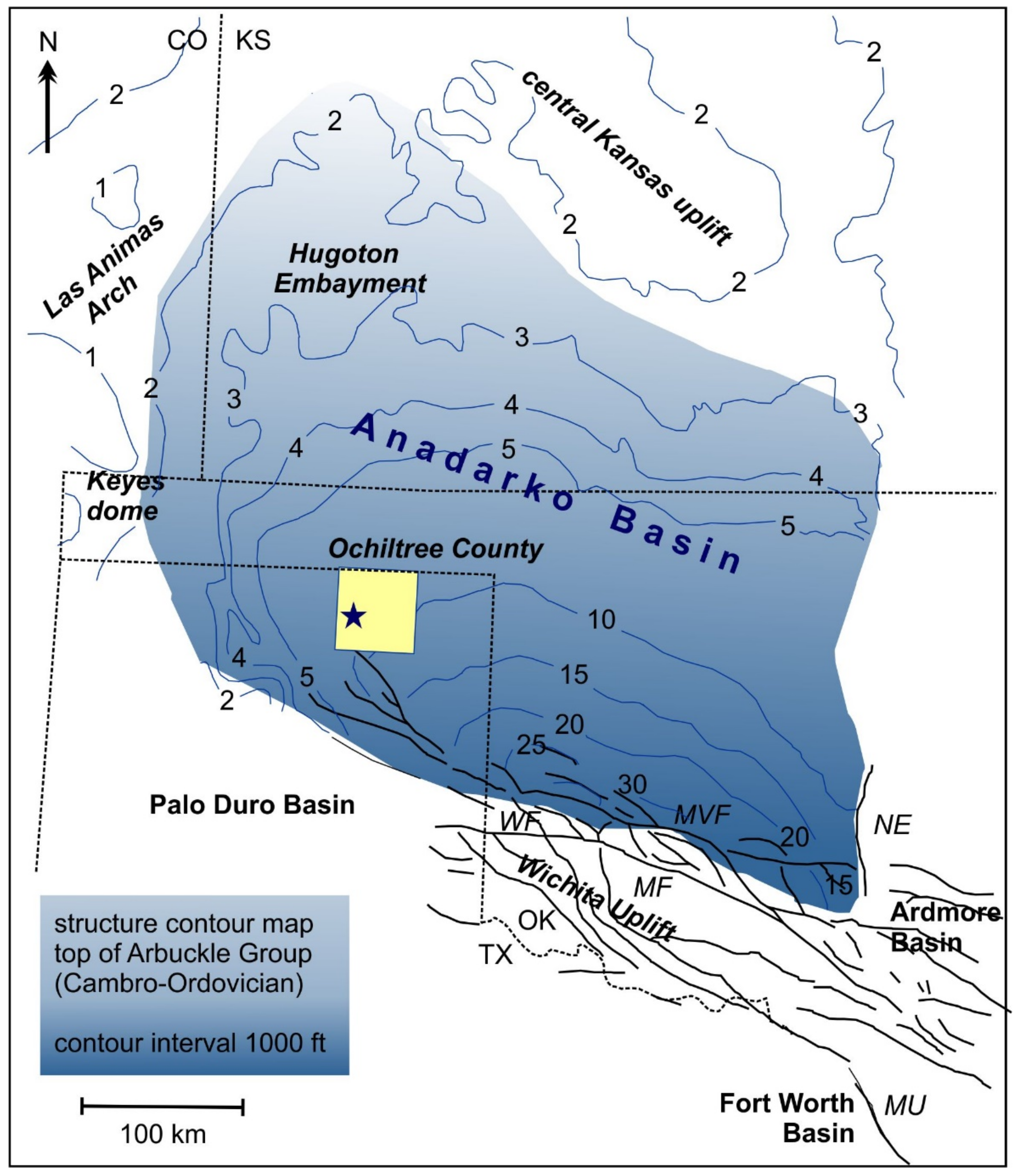
2. Anadarko Basin Overview

The Anadarko Basin is a mature, deep (as deep as ~12 km or ~40,000 ft, Figure 1) sedimentary basin in the North American craton that has been a prolific source of oil and gas since the early- to mid-1900s [17,18]. Its tectonic history starts in the Pre-Cambrian, and includes a series of orogenic and basin-forming events [17,18,19,20,21,22,23,24,25]. Pre-Cambrian basement rocks (Figure 3) consist of igneous and metasedimentary rocks emplaced in a basin of unknown origin [18]. In the Early- to Mid- Cambrian, a system of faults formed that has been interpreted either as indicating extensional deformation, or as a system of strike-slip faults [26], resulting in the Southern Oklahoma Aulacogen (a failed rift [17,25]. During this time, sedimentary and igneous rocks were emplaced in this basin [18]. Rifting ceased by Middle Cambrian time.
Subsequently, a phase of thermal subsidence occurred that led to the deposition of alternating carbonates, shales and sandstones in the Southern Oklahoma Trough [27]. These are the Arbuckle and Ellenburger Groups, deposited during the Middle Cambrian-Early Ordovician, mainly consisting of carbonates (Figure 3). The Simpson Group with sandy carbonates and clastic rocks was deposited in the Middle Ordovician, followed by the Late Ordovician Viola limestone and the Sylvan shale. The Silurian-Devonian Hunton Group mainly consists of shale and limestone; the Late Devonian- Early Mississippian Woodford Shale Formation overlays this group (Figure 3) [17,27,28,29,30,31,32,33,34,35]. Finally, the Woodford Shale was deposited; this is one of the source rocks for the Morrow B reservoir.
Flexural subsidence in the Anadarko Basin began in the Mississippian and continued through Late Pennsylvanian- Early Permian (Figure 3). From Middle Mississippian to Early Pennsylvanian (Morrowan), more than 2 km of sediments were deposited in the Anadarko Basin [36], including the Morrow B reservoir rock which is the focus of this study, and the Middle Pennsylvanian Kansas City Group located above the Atokan Thirteen Finger (cap rock for the Farnsworth Field petroleum system).
Cambrian through Mississippian sediments were deposited in large epicontinental sea environments and consist of a mixed clastic-carbonate system, siltstone, and shallow marine carbonate facies with minor sandstones and shales [18,36,37,38,39]. The Woodford Shale, one of the Anadarko’s major source rocks, was deposited during the Devonian; it thickens to over 375 ft in the basin center while pinching out along basin margins [16]. A pre-Pennsylvanian unconformity marks the contact between Mississippian and Pennsylvanian units and is present across most of the basin [21]. Paleo highs and lows during this time helped to control the deposition and drainage systems of early Pennsylvanian Morrowan incised valley fluvial systems [21].
Intrusive igneous Cambrian rocks were exposed south and southwest of the Anadarko basin as a result of Early to Middle Pennsylvanian tectonic activity, and are a source for Morrow B sandstones [40] as well as forming ‘granite wash’ deposits in proximity of the southern margin of the Anadarko Basin [41,42]. Subsidence of the Anadarko Basin slowed during Middle-Late Pennsylvanian. Pennsylvanian-Permian organic rich sediments deposited in the Anadarko Basin formed, together with the Woodford Shale, source rocks for the Farnsworth Field petroleum system according to our analysis (Section 5).
Strata of the Early Pennsylvanian Morrow B, which is the CO2 injection reservoir, are up to 4000 ft thick in the deepest southern part of the Anadarko Basin, and thin northward to less than 100 ft in the study site and on the shelf (Figure 3). Deeper Morrow strata consist of shallow marine shales, sandstones and limestones; Upper Morrow strata are shales, discontinuous sandstones, and deltaic deposits, see Figure 3 [18]. As discussed above, Morrowan deposits are the primary target interval for CO2 injection. An incised valley model is in agreement with the depositional character of many Morrowan fields, including Farnsworth Field [43,44,45,46,47,48,49,50,51,52,53]. The formation dips southeastward, and the Morrowan sandstones exhibit field-scale reflector offsets in seismic data that could indicate facies changes (discussed below).
Overlying the Morrowan rocks is the Thirteen Finger formation belonging to the Atokan deposits (Early Pennsylvanian) that forms the seal of the CO2 reservoir. They consist of marine shales, sandstones and limestones [18] (Figure 3). The seal directly overlying the Morrowan sandstone reservoir is the Morrowan black shale. It formed as sea levels rose along the basin margins [40]. Both the Morrowan and Thirteen Finger black shales contain appreciable TOC values [24]. The lower and Upper Morrow shales and Thirteen Finger Limestone form, together with the Woodford Shale, the source rocks for the Morrow B reservoir (Section 5). Timing of maturation of these source rocks is discussed in Section 5 of this manuscript.
Deposition of shales, carbonates and sandstones continued into the Triassic and Permian periods. The early Cenozoic Laramide Orogeny affected the Anadarko Basin by fault reactivation along the Wichita-Amarillo uplift, and tilted the basin eastward [19]. Additionally, associated epeirogenic uplift caused 1–3 km of erosion during the Cenozoic and brought the Anadarko into its present state. Cretaceous deposits in the basin have largely been eroded.

3. Subsurface Structure of the Western Anadarko Basin

Faults and fractures provide natural pathways for CO2 migration towards Earth’s surface. Regional and field-scale faults have been documented across the Oklahoma and Texas portions of the Anadarko Basin [54,55,56,57,58]. In the western Anadarko Basin, north of our study area in western Oklahoma, a NW-SE trending fault is reported in Beaver County [59]. In the Texas portion of the basin, a similar trending fault is inferred southeast of our study area [58]. Marsh and Holland [58] do not list faults in Farnsworth Field.
The potential presence of faults in proximity to the CO2 sequestration study area motivates further research on these possible CO2 migration pathways. Below, we discuss our interpretation of 2D legacy seismic data (Figure 2 and Figure 4), that allow us to search for faults directly east and north of Farnsworth Field, as well as an interpretation of 3D seismic data of the Farnsworth Field study site (Figure 5, Figure 6, Figure 7).

3.1. Interpretation of 2D Seismic Lines

The SWP purchased over 100 miles of 2D legacy seismic data from Seismic Exchange Inc. covering an area from near Farnsworth Field to the east and southeast (locations shown in Figure 2). The 2D lines were acquired by Seisdata Services, Inc. from 1984 to 1986 and all sources were generated by Vibroseis except for line DC-NEP-10 which was generated using Primacord. The lines were reprocessed in 2014 by Seismic Exchange, Inc. Interpretations from Gragg [60] (interpreted lines DC-NEP-10 and DC-NEP-33) are shown in Figure 4. Mis-tie corrections were applied to crossing 2D lines to account for the inconsistencies in quality, static solutions, and vintages [60]. A seismic well tie was made from the Killingsworth well because it had sonic and density logs, a checkshot from surface to approximately 8600 ft., and was close to the seismic line [60]. Gragg [60] constructed a velocity model from the Killingsworth well tie, and the seismic lines were converted to the depth domain. The interpreted 2D seismic data also provided the geometry input for the petroleum system model (Section 5).
Formations generally dip southeastward in our study area, which is in agreement with regional trends [22,61,62]. The dip increases with stratigraphic age and units tend to thicken toward the deep basin. The Atokan and Morrowan formations are continuous, relatively transparent seismically, and cannot be resolved individually on these low-resolution lines. The top Mississippian is interpreted as an angular erosional unconformity, formed as a result of the Wichita orogeny [24]. There are no indications for faulting or seismic chimneys in both the east–west and north–south lines in the Atokan and Morrowan formations.

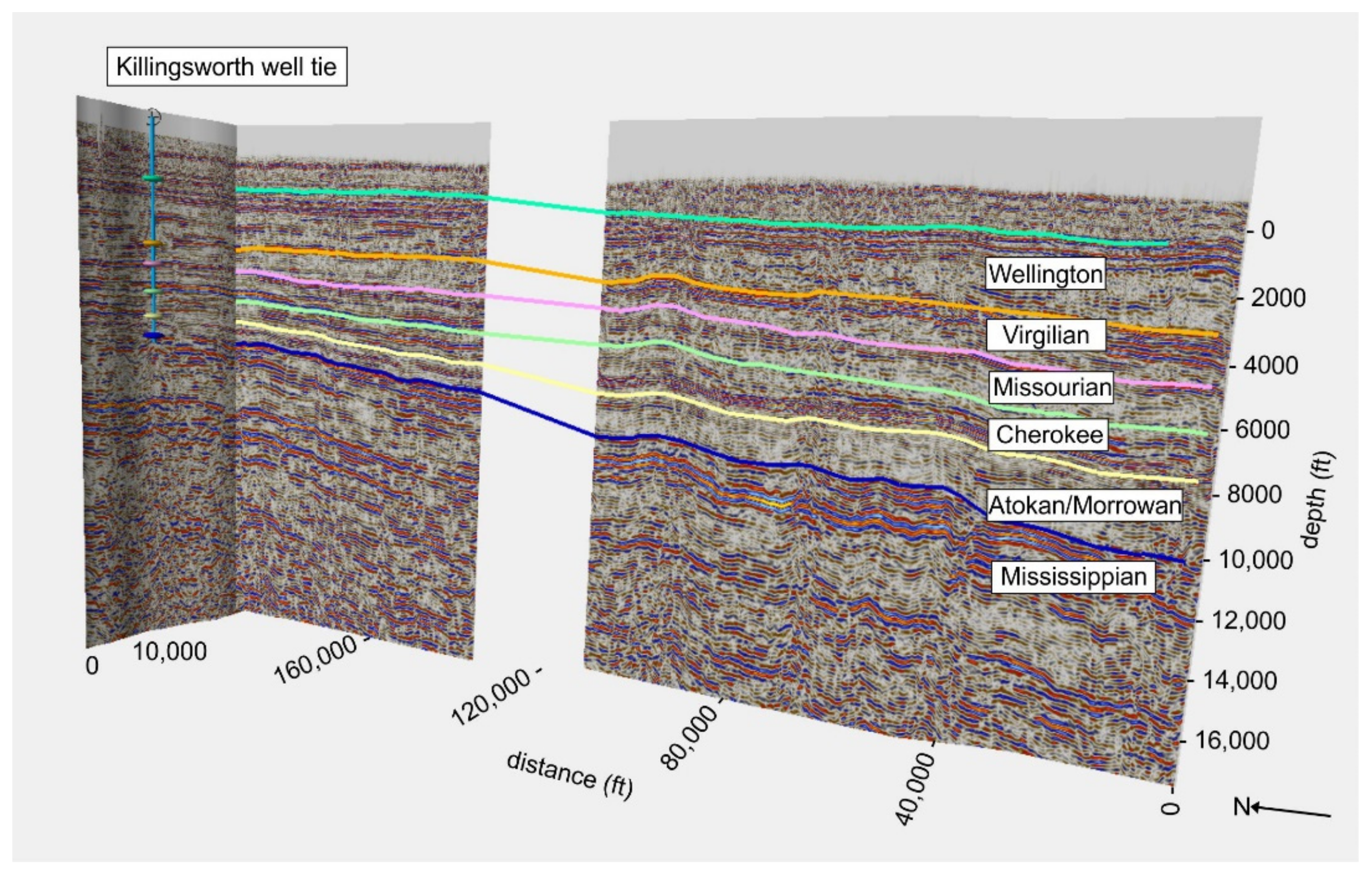
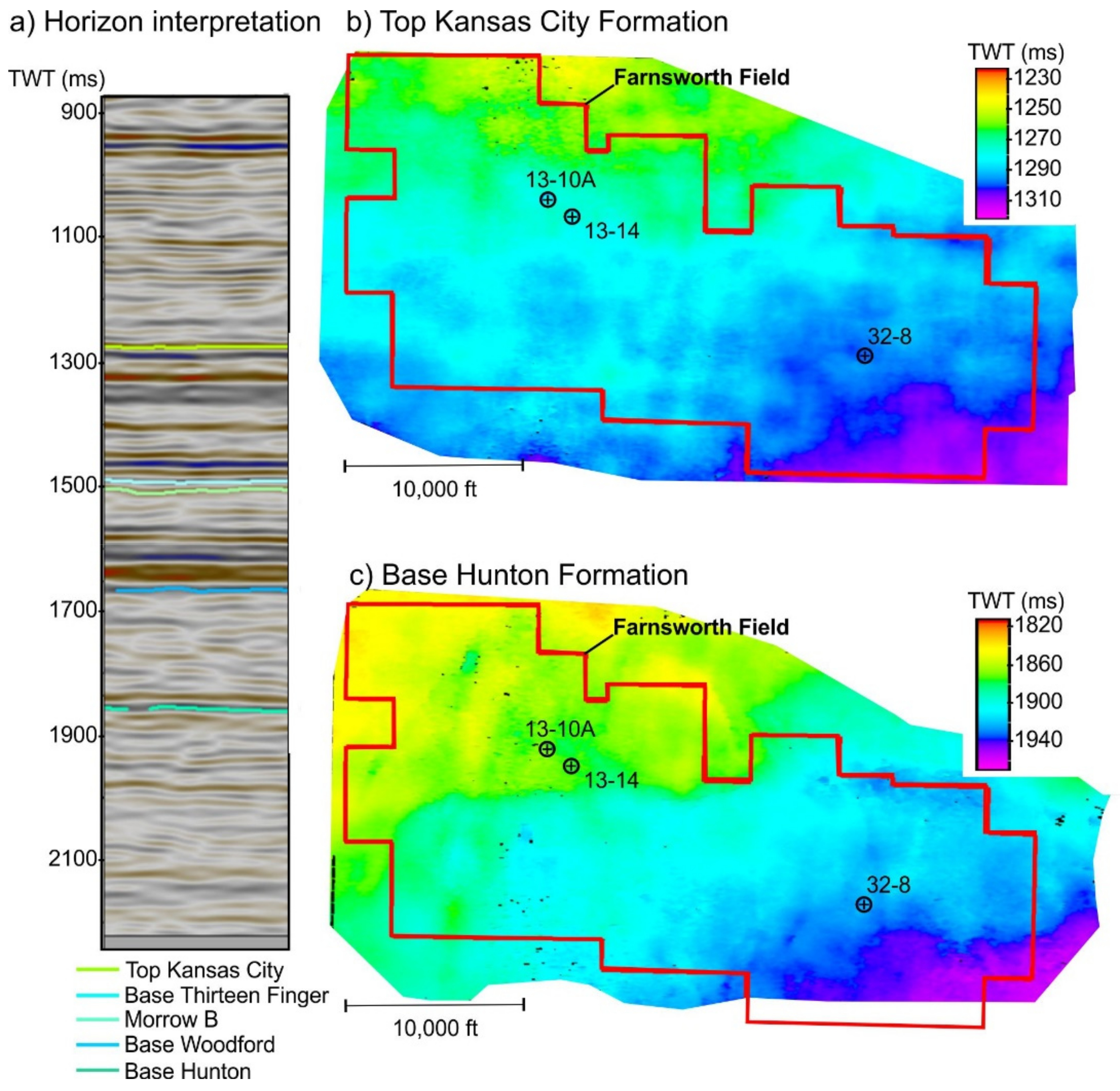
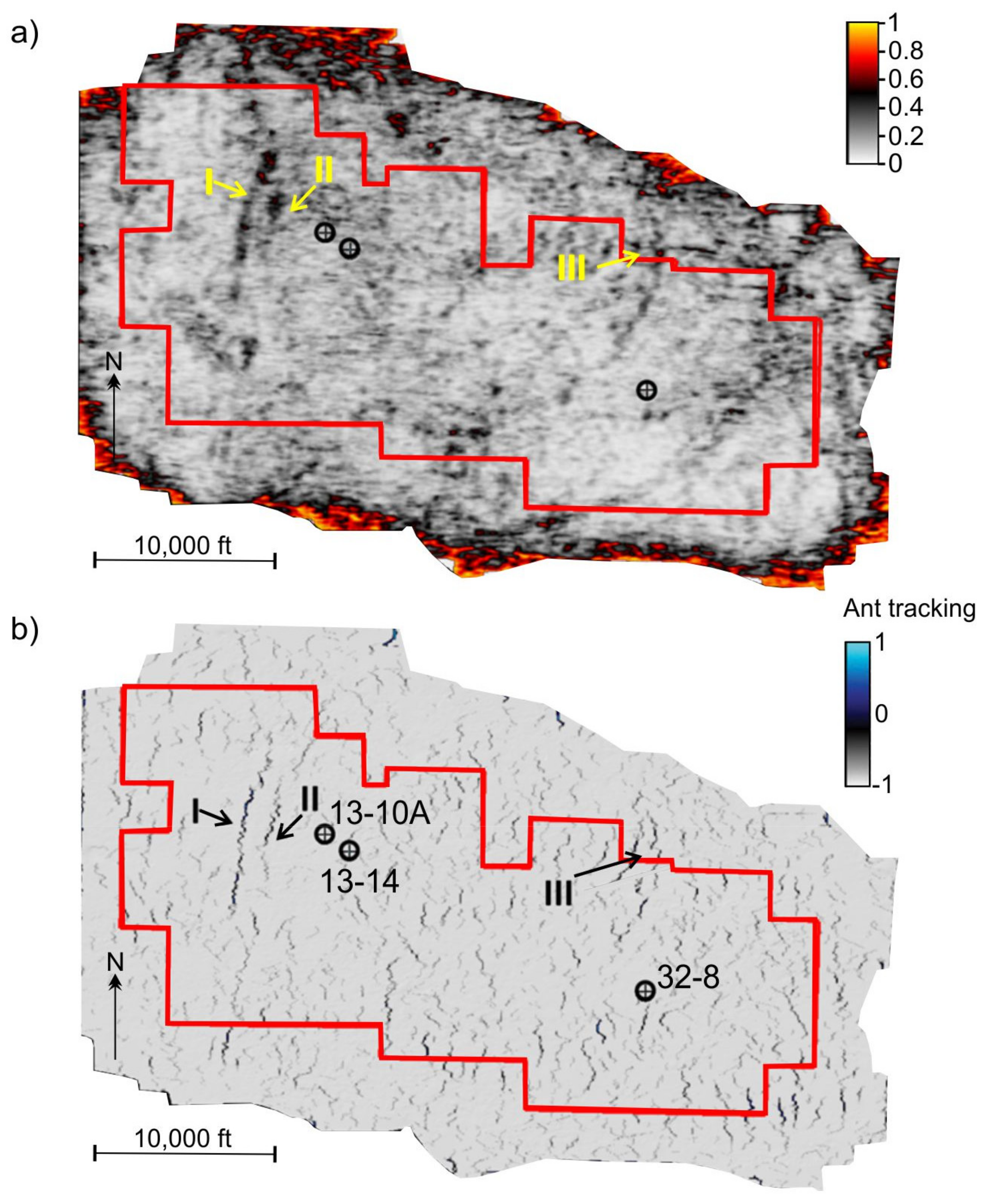
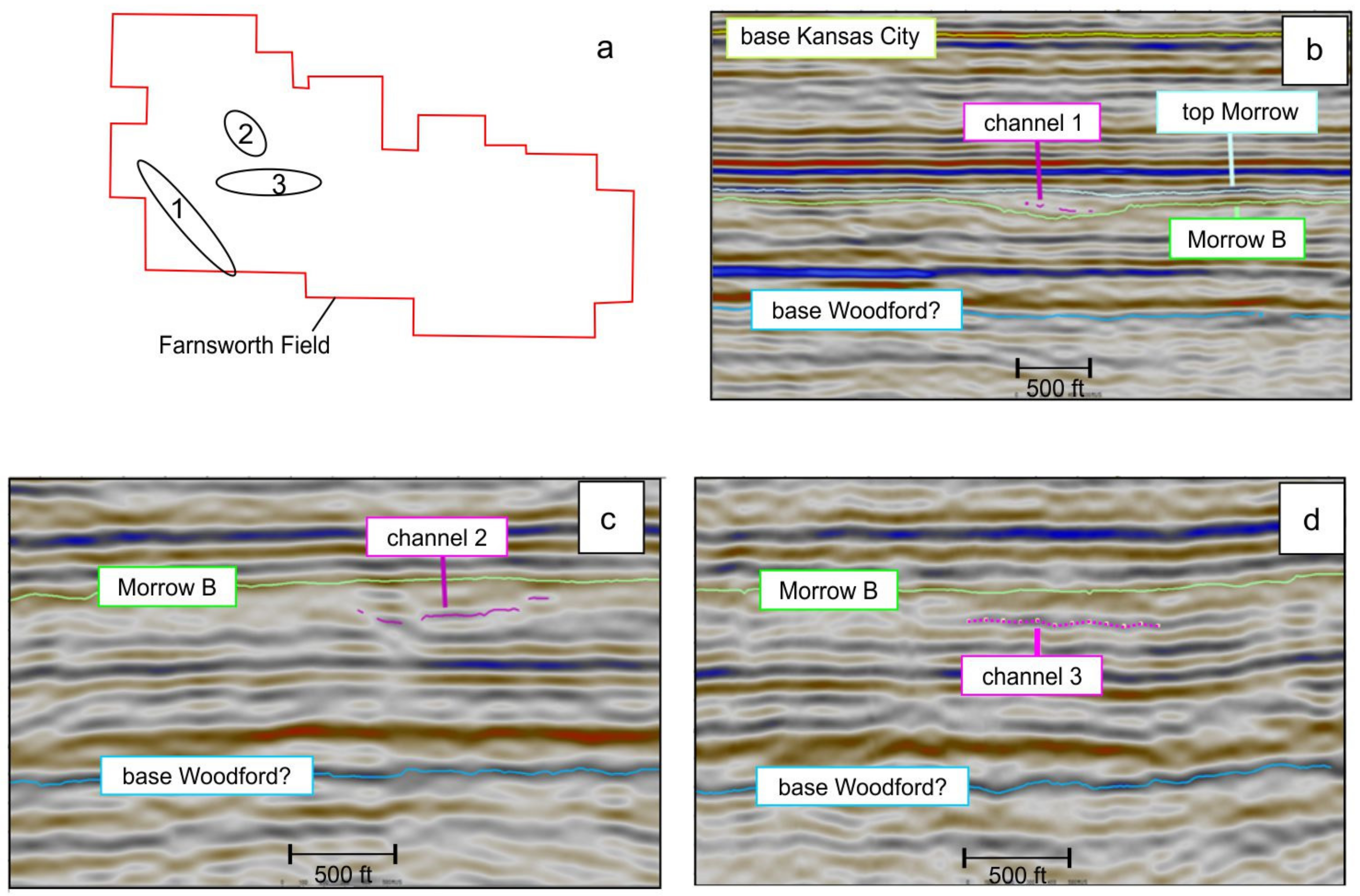
3.2. Interpretation of 3D Seismic Survey

3D Reflection seismic data (Figure 2, Figure 5 and Figure 6) were acquired in 2013 by SWP through WesternGeco over an approximately 42 mi2 surface area, with full fold covering 27 mi2. The geophones had 33 ft. spacing and dense vibroseis source points with a sweep frequency of 2–100 Hz. Processing steps and survey characteristics are described by [63]. Preliminary interpretations of this dataset suggested that the Morrow B reservoir could be faulted, with faults striking E, S, and SE [64]. Our interpretations show that the seismic discontinuities that were interpreted as faults in White et al. [64] are erosional features, incised channels, and karst structures.
Wells 13-10A and 32-8 (locations shown in Figure 5) were used for well ties. The Morrow B reservoir rock reaches a maximum thickness of ~70 ft in Farnsworth Field, and its boundaries cannot be resolved in the seismic data. Since the exact location of the Morrow B horizon in the seismic data is thus uncertain, a reflector in the proximity of the Morrow B (Figure 5a) was traced confidently in the seismic data. In further analyses, we used an isopach map of the Morrow B that we created from interpolation of 346 well logs. Figure 5 shows the position of the Morrow B reservoir layer with respect to the overlaying Thirteen Finger Limestone and Kansas City Group, and the underlying Woodford and Hunton Formations. In Farnsworth Field, paleozoic formations dip slightly toward the southeast (Figure 6).
We applied several seismic attributes [65,66,67] to the 3D seismic dataset to detect faults and fractures that may act as migration pathways for sequestered CO2. Seismic attributes were used to help identify features such as fractures, faults, and stratigraphic changes that may not be easily discerned in the original data. We generated edge-detection attributes that measure waveform similarity (Variance and Amplitude Contrast) and Ant Tracking volumes that track continuous features in an effort to illuminate possible fault structures. Parameters were varied within Petrel® software to best highlight any discontinuities while keeping the parameters in a reasonable range.
Variance is an edge enhancement attribute used to estimate localized variance in the seismic signal [65]. The Amplitude Contrast attribute analyzes derivatives in all three components [66]. Petrel® software 2017 allows the user to apply dip corrections, vertical smoothing filters, and the ability to steer the volume along an azimuth. The default values resulted in the best results, as discussed below. The edge detection attribute Ant Tracking uses either the Amplitude Contrast or Variance volumes as input. The attribute attempts to improve the signal-to-noise ratio of discontinuities. To generate the best Ant Tracking volume for highlighting discontinuities, multiple variations of Variance and Amplitude Contrast volumes were generated.
The edge-detection attributes did not illuminate any features that could be interpreted as faults (Figure 6). We did identify channels, a karst-collapse structure, and erosional features; these are discussed next.
We identified an elongated area associated with north–south trending linear features visible in the Variance and Ant Tracking volumes (discontinuities I and II in Figure 6), which were previously interpreted as faults [64]. In the Variance volume, the N-S features bounding this area appear wide (approximately 100 to 1000 ft. wide) while they look sharp in the Ant Tracking volume (Figure 6). Two vertical cross sections through this feature (Figure 7) illustrate that this is probably caused by differential compaction of shales above an erosional feature in the Hunton limestone that developed prior to the deposition of the overlying horizon (which has tentatively been marked “Woodford”). This resulted in draping over the deeper structure. The Ant Tracking discontinuities and the wide banding on the Variance volume likely identified changes in the seismic signature. Surfaces interpolated from well-logs supported this interpretation; a small gradient that is compatible with draping, and vertical offsets are only about 9 ft to 48 ft at the top of the Morrow B [56].
The second structure that we discuss here is the feature on the edge of the NE side of the field (Figure 7c). This feature appears very faintly on the Variance cube (Figure 6a, indicated with III), and does not appear on the Ant Tracking attribute (Figure 6b). This feature was interpreted as an E-striking fault in White et al. [64]. Offset of the top of the Morrow B directly above this feature, based on well log tops, is approximately 30 to 60 ft. The feature could be identified easily as a pronounced down-warping of the Morrowan, Atokan, and basal Woodford reflectors. We interpreted this as a karst collapse structure. The collapse structure possibly formed in the Hunton limestone during a period of low sea level.
We have identified several channel features (Figure 8) in the western Farnsworth Field area. Our interpretation is consistent with the incised valley model proposed by Krystinik and Blakeney [44] in which the Morrow B sandstones were deposited in incised valleys on the basin margin as the sea level rose. Although not resolvable with the 3D seismic data, it is possible that such facies changes or channels could form preferential flow paths for CO2. The channel in Figure 8b is particularly well defined, but most of the reflectors that could be identified as channel fills seem laterally discontinuous (Figure 8c,d). This is due to the fact that the thickness of many of these channel infills is below the 3D seismic resolution.
The Kansas City Formation, Morrow B, and Woodford Formation drop down a few tens of ft southward in the center of Farnsworth Field (Figure 5). They drape over an erosional edge in the Hunton limestone, which was previously interpreted as an east-striking fault (fault #3 in White et al., 2017, their Figure 3).
We were not able to identify faults in the Morrow B or overlying formations. We note that this does not necessarily mean that faults and fractures are not present, but they can simply not be resolved with our seismic datasets. To understand possible flow paths for CO2 within the Morrow B, and between the Morrow B and surrounding formations, we will compare our interpretations of the Morrow B to results of a tracer study and with a petroleum modeling study.

4. Flow Paths in the CO2 Reservoir

Seal analyses of the Morrow B and Thirteen-Finger Limestone Formations [68] suggest that upward CO2 migration through the seal, by flow through permeable pathways or stress-induced breakage of the seal, is unlikely in Farnsworth Field. The absence of detectable faults in the Morrow B and overlying formations suggests that no major fault zones are present along which CO2 could migrate. Here, we discuss lateral migration through the Morrow B reservoir.
Aqueous-phase tracer studies were conducted in the western half of Farnsworth Field in 2014, 2015, and 2017. Naphthalene sulfonates were injected in wells 13-3 (2017), 13-5 (2014), 13-10A (2014), 13-13 (2014), and 14-1 (2015), Figure 9, Figure 10, Figure 11. These are a family of organic compounds that have successfully been used as tracers in geothermal and petroleum reservoirs [69,70,71,72,73], and ground water studies [74].

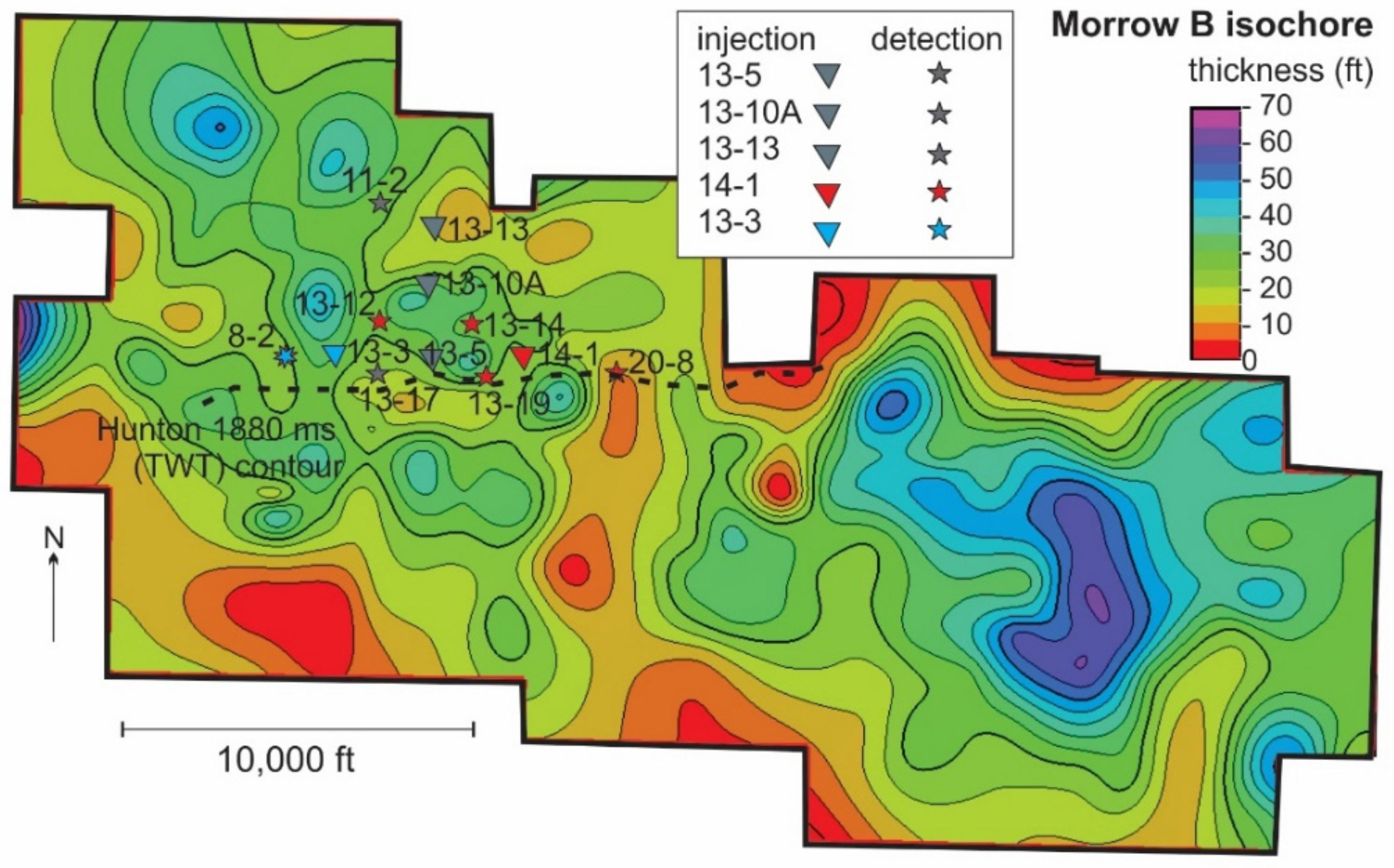
4.1. Tracer Study Setup

The naphthalene sulfonate compounds that were used as tracers in this study were obtained from YickVic Chemicals, Hong Kong, China. The three tracer tests described below were initiated between May 2014 and June 2017, with sampling and analysis continuing into 2018. In each case, a concentrated aqueous solution (~5%) of a naphthalene sulfonate was mixed with fresh water at the wellhead and injected as a slug over a duration of approximately 0.5 h. Table 1 summarizes the tracer injection scheme.
The surrounding production wells were sampled over the subsequent four years for tracer analysis by High-Performance Liquid Chromatography (HPLC) and fluorescence detection with detection limits of approximately 100 parts per trillion [68,69]. In order to separate matrix interferences from the tracer analytes, the samples were subjected to solid phase extraction prior to analysis. Decay kinetics studies have shown that all of the naphthalene sulfonate compounds used in this study are suitable for use in geothermal reservoirs having temperatures up to 250 °C, and a subset are suitable for use in reservoirs as hot as 300 °C [68,69,70,71,72].

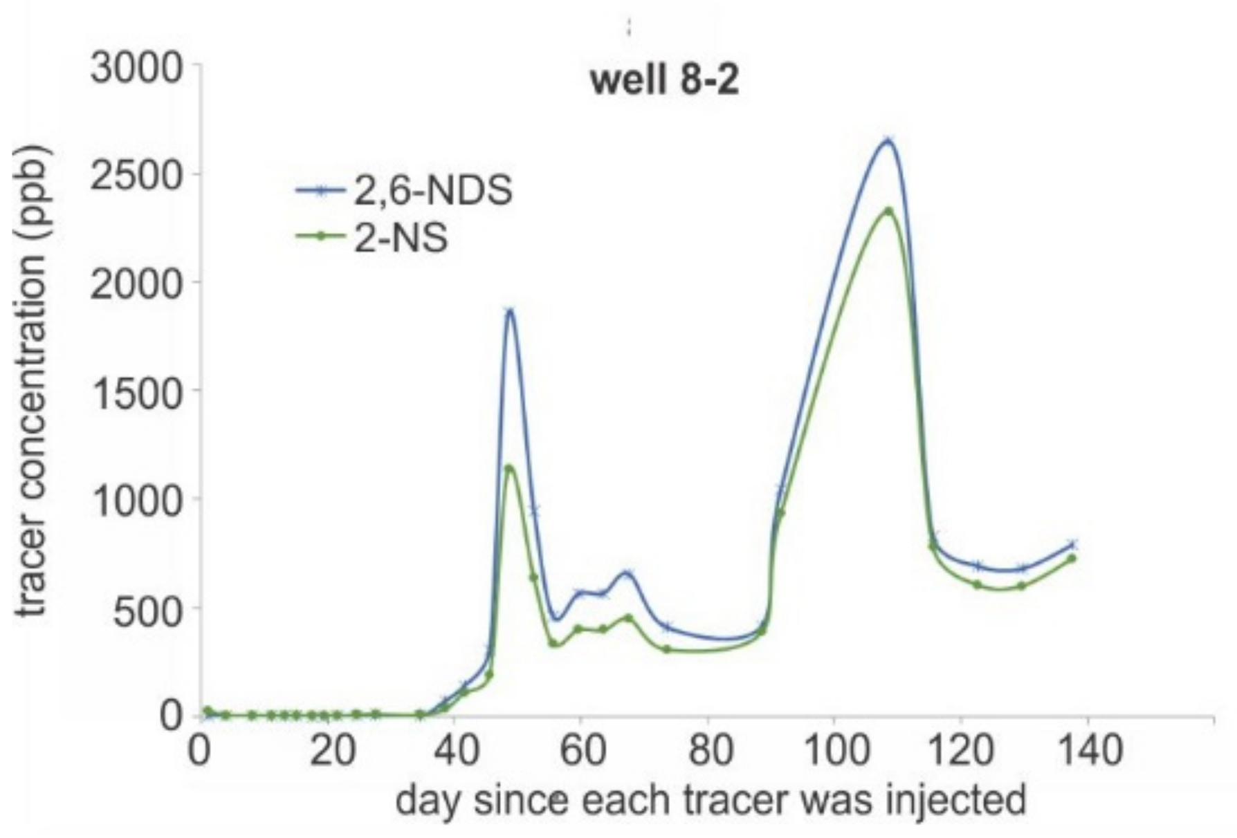
4.2. Tracer Study Results

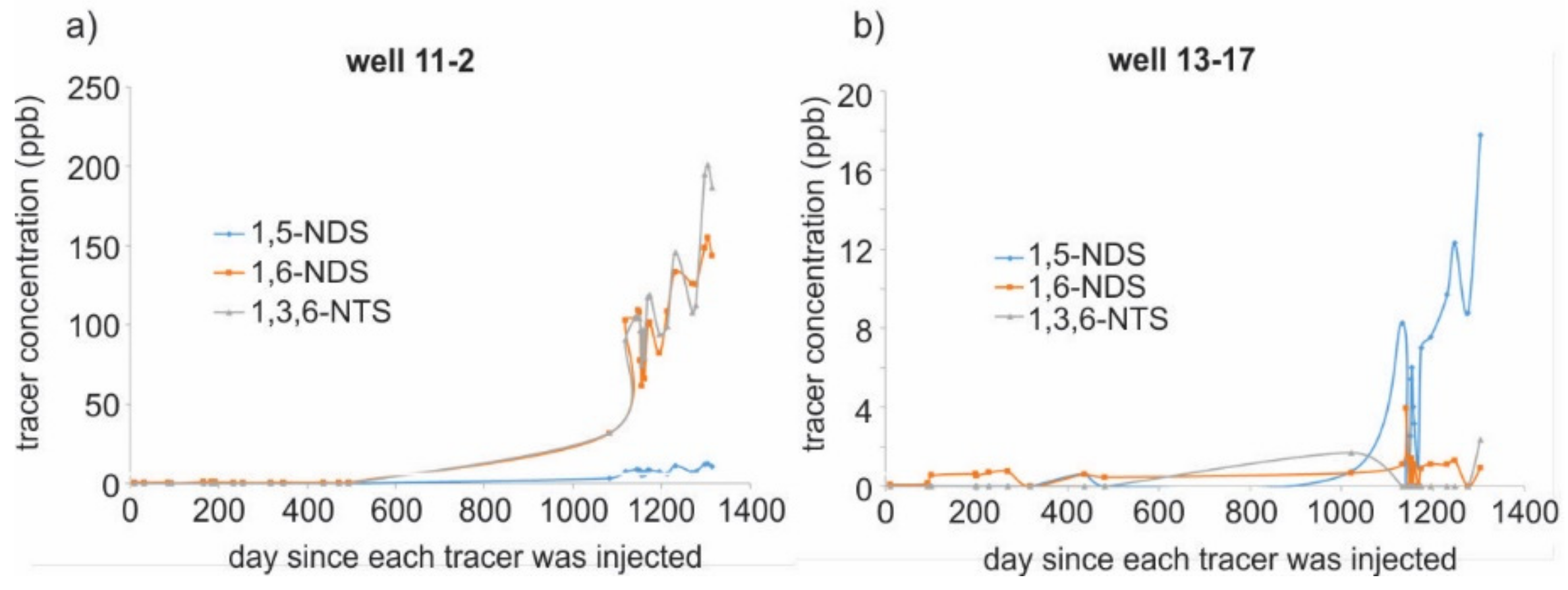
4.2.1. Tracer Tests of WAG Injection Wells 13-13, 13-10A, and 13-5

On 2 May 2014, 27.5 kg of 1,6-naphthalene disulfonate (1,6-nds); 50 kg of 1,3,6-naphthalene trisulfonate (1,3,6-nts); and 25 kg of 1,5-naphthalene disulfonate (1,5-nds) were each mixed with water and injected into the three injection wells 13-13, 13-10A, and 13-5, respectively. All three wells were receiving alternating injections of water and CO2. The aqueous phase of all surrounding wells was sampled regularly over the subsequent four years and analyzed for the presence of the naphthalene sulfonate tracers.
The well showing the most significant returns of the three tracers was 11-2 (Figure 9). Due to a long sampling hiatus between about day 500 and day 1100, it is not known when breakthrough first occurred. However, given the shape of the curve, it was probably not before about day 1000. Thus, it was almost three years before the tracers injected into wells 13-13, 13-10A, and 13-5 broke through to the northeast well 11-2. A second well showing returns of tracers injected during the 2014 test was 13-17. The other two tracers in which tracer was injected in 2014 showed negligible concentrations in 13-17.

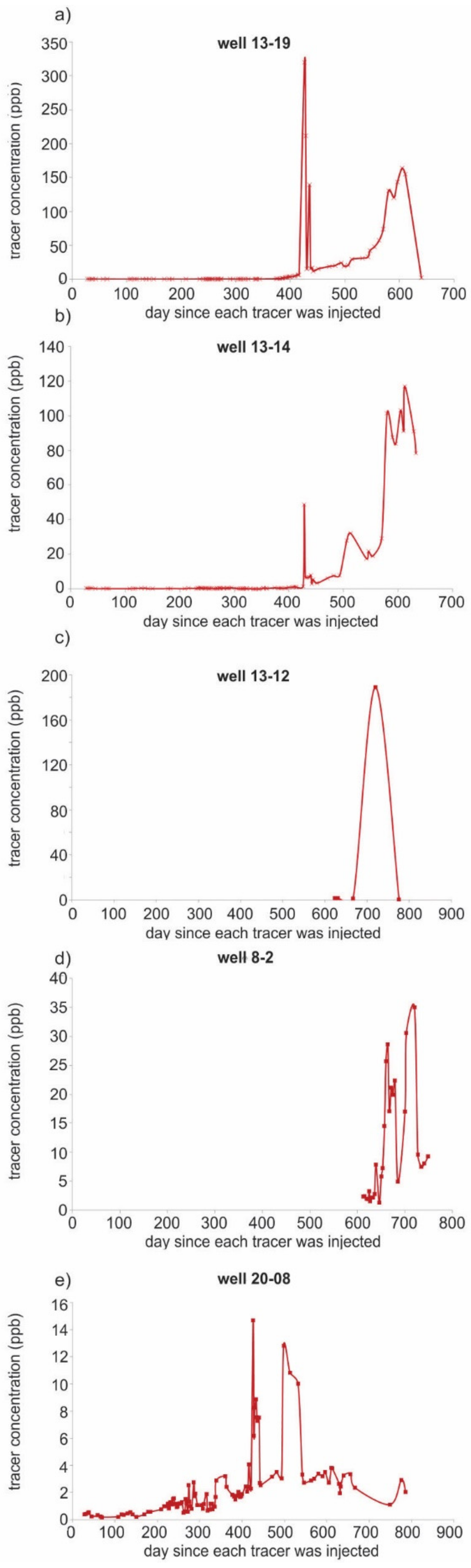
4.2.2. Tracer Test of Water-Injection Well 14-1

On 13 October 2015, 100 kg of 2,7-nds was mixed with water and injected as a slug into water-injection well 14-1. Surrounding production wells were sampled and analyzed over the subsequent 2.5 years. Figure 10 shows the return curves for the wells that showed tracer returns.

4.2.3. Tracer Test of WAG Injection Well 13-3

On 15 June 2017, 100 kg of 2,6-nds and 80 kg of 2-ns were mixed with water and injected as a pulse into well 13-3. The surrounding wells were sampled over the subsequent six months, but the only well showing returns was 8-2, which is located directly west of 13-3. Shown in Figure 11 are the very strong returns of these tracers to 8-2.

4.3. Discussion: Interpretation of Tracer Study Results

The line of wells running north to south near the middle of the study site (13-13, 13-10A, and 13-5) were all tagged in May 2014. These three wells were subjected to water-alternating-gas (WAG), whereby brine would be injected for a few weeks followed by the injection of CO2 for a few weeks. The first arrivals of tracer were all approximately 1000 days after injection in spite of the fact that the distances between wellheads varied significantly. In the case of well 13-5, the first arrival of tracer was approximately the same for tracer arriving at adjacent well 13-17 as it was for the much more distal well 11-2. In contrast, the first arrival of tracer injected into well 14-1 was never more than 625 days in spite of traveling a greater distance—at least in the case of well 8-2. This difference in aqueous-phase flow velocity might be explained by the fact that 14-1 was never subjected to WAG but was only on water injection. In the case of well 13-3, the first arrival time to adjacent well 8-2 was much shorter (~40 days) with concentrations that were more than 10 times greater than those of any of the other tracers. The two peaks in this return curve (Figure 11), with maxima at 50 and 110 days reveal the very heterogeneous flow patterns between this pair of wells. Flow heterogeneity was likewise observed in many of the other return–curve plots (Figure 9 and Figure 10).
Although we have only a limited number of datapoints available, a well-to-well flow pattern can be recognized. Flow of the tracers is generally west to northwest, except for tracers injected into well 14-1, which were also detected toward the east of the injection well (Figure 12). Close inspection of the depth of the Morrow B reservoir in and between these well locations suggests that inter-well flow occurs between wells where the Morrow B is at the same depth, or in an up-dip direction; all wells where tracers were detected are up-dip from the injection wells. The Morrow B isochore map (Figure 12) shows that the Morrow B is of irregular thickness, and locally thins significantly just south of wells 13-17 and 13-19. The Morrow B deepens southward along an approximately EW-striking “step” (previously interpreted as fault #3 [64]), and drapes over the deeper Woodford and Hunton formations; the Hunton formation is locally eroded. It is possible that tracers injected north of the step (indicated with the dashed contour in Figure 12) in the Morrow B will not flow south of this step. If inter-well flow is horizontal or up-dip, the impermeable cap rock of the Morrow B (Thirteen Finger) would prohibit down-dip, or (generally) southeastward flow from the tracer injection wells, since the step in Morrow B depth is of the same magnitude as the thickness of the Morrow B.
This interpretation differs from earlier preliminary work that ascribed inter-well flow directions to presumed faults in the Morrow B [64]; our updated interpretations discussed above suggest that erosional features play a role in inter well flow. The seismic data do not provide sufficient resolution to link flow directions with incised valleys.

5. Petroleum System Model of the Farnsworth Petroleum Field

Higley [16] developed a 4D petroleum system model of the Mississippian-Pennsylvanian petroleum system in the Anadarko Basin, and found that present and past oil-migration flow paths in the Texas Panhandle are directed SE-NW, sourced in the deep portion of the Anadarko Basin, where Transformation Ratios are close to 1 [16,75]. Petroleum in Farnsworth Field is likely commingled [75], and sourced from four distinct families of oil (Ordovician-Viola, Woodford, Morrow, and Upper Pennsylvanian). Migration paths may be over 100 km long [16,75]. In the Farnsworth Field, distribution of oil accumulation is controlled by the Morrow incised valley complex.
Basin-scale studies of the Anadarko basin [16] provide insight into the petroleum system of the basin but do not provide detailed insight into petroleum sources and migration paths for our study site. To fill this gap, we developed a 2D petroleum system model of the Farnsworth Field region with Schlumberger PetroMod® (2013) software. We also constructed a burial history curve to understand the time-depth relation of the cap rock (Thirteen Finger Limestone formation).

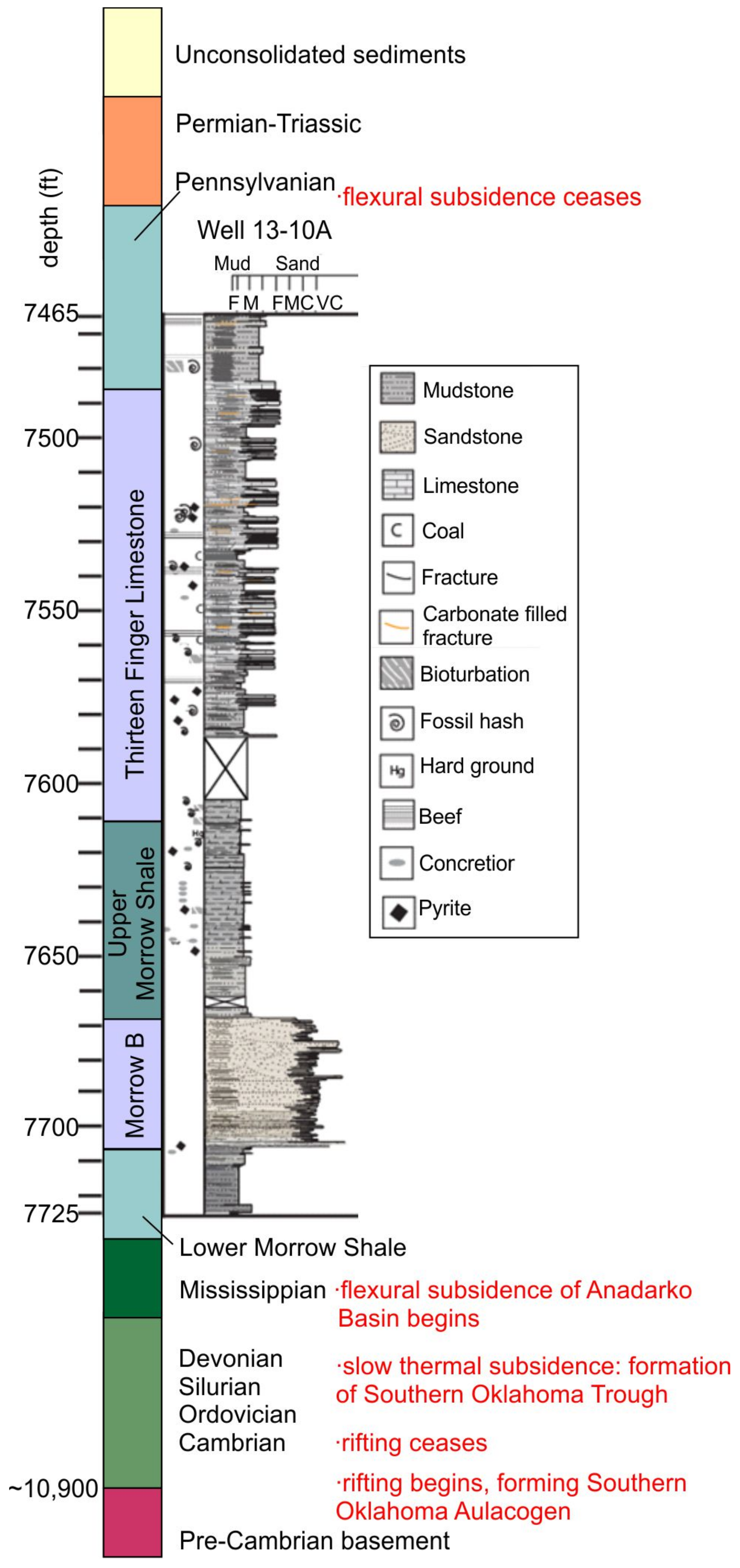
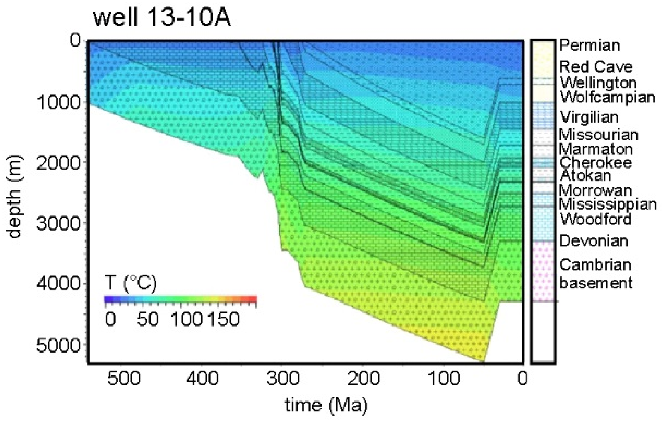
5.1. Setup of 1D Petroleum System Models

A burial history curve was constructed for well 13-10A (Figure 13 and Figure 14, Table 2). Sixteen stratigraphic units and basement were included as a unit in the 1D petroleum system model. Each unit was assigned lithofacies information (Table 2), thickness, age of deposition, and, if appropriate, age of erosion. Each unit was also assigned its role in the petroleum system (source, reservoir, seal, underburden, or overburden). Four source rocks were included: the Woodford shale, lower Morrowan shale, Upper Morrowan shale, and Thirteen Finger Limestone. Each source rock was assigned a hydrogen index (HI), total organic carbon percentage (TOC), and a kinetics model. Lithofacies were generalized based on SWP well log and core data; TOC and HI values are from SWP core analyses.
Geologic ages of the different formations (Table 2) are based on Higley et al. [62]. All lithologies were generalized based on the dominant lithology present within a model layer. Erosion amounts and timing for the pre-Pennsylvanian unconformity were based on interpretations of the unconformity being regional [21]. Well log data of well 13-10A did not reach basement depths because operators were not targeting intervals below the Morrowan Formation. In order to include the complete Anadarko Basin’s burial history, the modeled wells were extended to basement using 2D seismic data. The top of the basement in the seismic data has a distinctive seismic character change from sub-parallel laterally continuous reflectors to chaotic discontinuous reflectors. Basement depths were obtained by performing a seismic well-tie, and used a velocity model for the depth conversion, as described above. Once the seismic data were depth-converted, depth estimates for the Woodford Shale, Cambrian-Devonian, and basement were added to the one-dimensional and two-dimensional models. The Woodford Shale depth, thickness (40 ft), and initial TOC (~1.5–2%) were approximated from Higley et al. [62]
We constrained the burial history curve and basin thermal history with vitrinite reflectance, production data, and Rock-Eval pyrolysis data [60]. Schlumberger PetroMod® software was used to predict temperatures in the well, and we calibrated those temperatures with thermal maturity indicators. As an example, the well 13-10A 1D petroleum system model predicts a Morrowan reservoir temperature of 74 °C and a maximum reservoir temperature of 104 °C that occurred around 50 Ma (Figure 13). Hinds [76] documented the actual reservoir temperature of Farnsworth at time of discovery as 75.5 °C (168 F), similar to our predicted value. The resulting burial history curve is shown in Figure 13.

5.2. Results of 1D Petroleum System Modeling

Slow subsidence with intermittent periods of uplift characterized the pre- Late-Pennsylvanian history of the western Anadarko Basin (Figure 13). A phase of relatively rapid subsidence occurred during the Late Pennsylvanian- Early Permian, when the Anadarko Basin subsidence accelerated as part of foreland basin development [22,27,43,62,77]. Subsidence continued until the start of the Laramide orogeny. Temperatures increased to about 130 °C in the deepest part of the column (Figure 13) until the onset of the Laramide deformation. In agreement with previous studies [16], our 1D model predicts that the Woodford Shale, Morrowan Formations, and the Thirteen Finger Limestone are currently in the oil and gas windows.

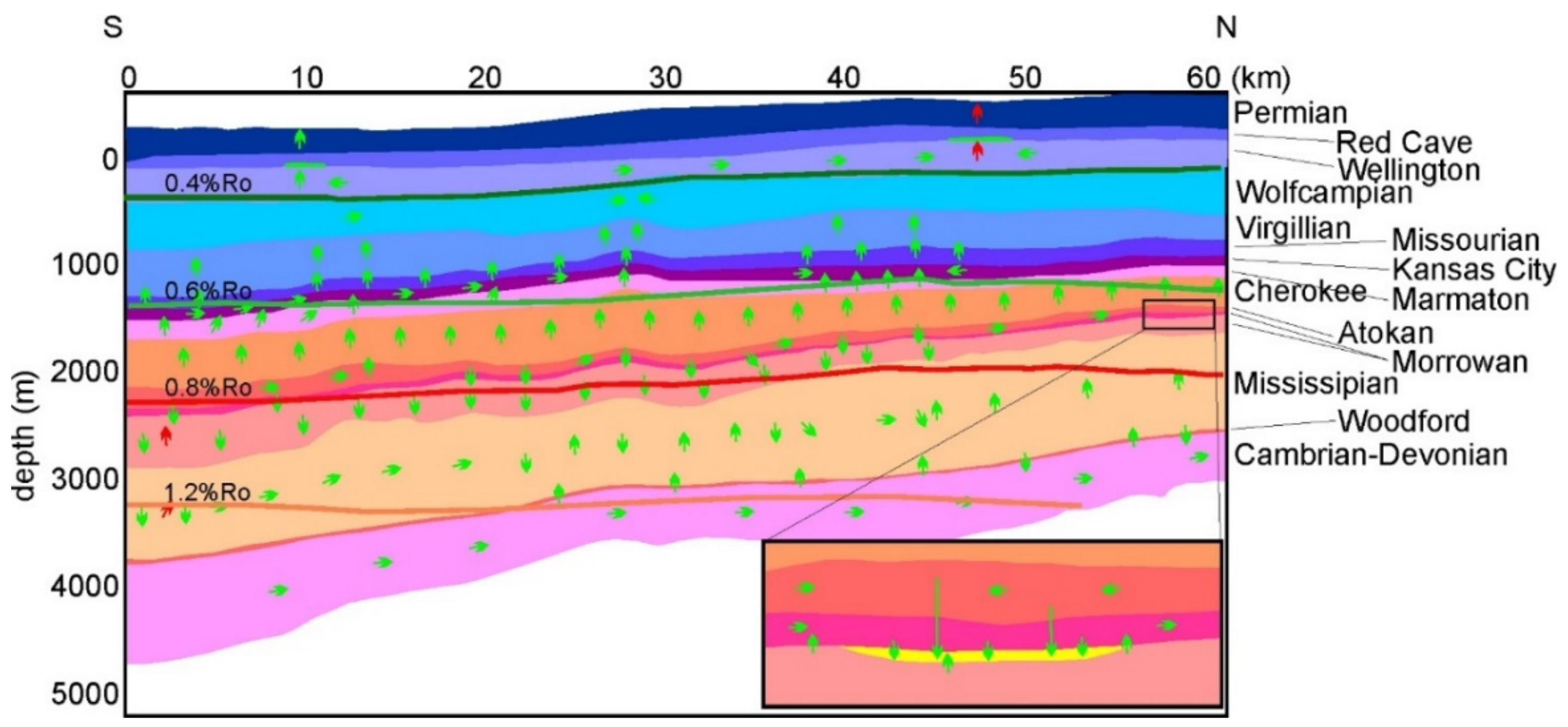
5.3. 2D Petroleum System Modeling Setup

Interpreted seismic line DC-NEP-33 (north and south, Figure 4) provides the depths and geometries for the layers in our 2D petroleum system model. The 2D petroleum system model gives insight into petroleum migration and paleo-leakage pathways, and allows for more detailed analysis of fluid accumulations and compositions in the region than the 1D analysis. Only thicker sedimentary sequences or packages (hundreds of meters) were included in the petroleum system models, except around the Morrowan reservoir of interest where layers decrease to thicknesses of tens of meters. Two erosional events were modeled: the pre-Pennsylvanian subsurface unconformity and Laramide uplift and erosion (Table 2). The pre-Pennsylvanian unconformity is present across the NE Texas Panhandle [21,46]. In our study area, the unconformity associated with the Laramide uplift is at the surface, where 1–3 km of Mesozoic and Permian deposits have been eroded as the basin was tilted eastward in the Cenozoic [54,60].
The Booker Field (location in Figure 1) well logs indicate a reservoir sandstone facies that is not resolvable on the 2D legacy seismic lines; this was included in the 2D model as it is an important reservoir rock. Dimensions of this sand body are estimated from SWP well logs and literature [44,60]. This sandstone body is the active injection interval for CO2-EOR operations at Booker Field. Figure 14 shows formations and corresponding depositional ages of the 2D model.

5.4. Results of 2D Petroleum System Modeling

The 2D petroleum system models predict hydrocarbon accumulation and fluid properties (Figure 15). The Behar et al. [78] type II compositional kinetic model was selected for the Thirteen Finger Limestone and Upper Morrow shale; the Behar et al. [78] type III compositional kinetic model was selected for the lower Morrow shale, and the Lewan and Ruble [79] Woodford shale hydrous pyrolysis kinetics model was used for the Woodford shale (Table 2). We selected the hybrid Darcy/flowpath model to describe petroleum flow in Schlumberger PetroMod® software.
Modeled temperatures in the Morrowan formations increase southward along line DC-NEP-33 from 70 °C to 105 °C. The model predicts that the CO2 reservoir is presently at 74 °C at the locations of Farnsworth and Booker Fields. The Thirteen Finger Formation temperature ranges from 67.5 °C to 87 °C. This southward increase in temperature is reflected in the basin’s maturation; maturation within a formation generally increases southward (Figure 15). In our modeled transect, the Woodford Shale is most mature, and its predicted vitrinite reflectance is between 1–1.3% Ro; vitrinite reflectance of the Atokan Thirteen Finger is between 0.65–0.8% Ro. In our models, only the deep Woodford Shale is in the gas window. This formation has a Transformation Ratio of 100% in the south, and 42% in the far-north part of the section. The Thirteen Finger’s Transformation Ratio ranges from 30.5–6%, the Upper Morrow Shale from 40–7%, and the lower Morrow Shale from 33–1.3% (south to north; Transformation Ratios are lower in the north). Even though the Transformation Ratio of the lower Morrow Shale is high, it generates low volumes of hydrocarbons in our model because the organic carbon content is low.
In our model, hydrocarbons were expelled from the Woodford Shale from c. 301 Ma in the southern part of the section and around 206 Ma in the northern part. The lower Morrow Shale is the next deepest potential source layer but does not indicate hydrocarbon expulsion onset anywhere. This is explained by its low hydrogen index of 10 (Table 2). The expulsion onset for the Upper Morrow Shale is at 270 Ma in the south and 125 Ma in the north. The Thirteen Finger has expulsion onsets at 299 Ma and 260 Ma in the south and north, respectively. Hydrocarbon migration pathways (Figure 15) are generally vertical and up-dip northward, with some exceptions; primary migration is locally downward, and the Morrowan sandstone reservoir is charged by the Upper Morrow shale, the Woodford (through the Lower Morrow shale), and the Thirteen Finger Limestone (Figure 15).
Migration in the Thirteen Finger Limestone began around 299 Ma along the section. Migration paths contain both vertical and lateral pathways as hydrocarbons meet resistance from low permeability strata (Figure 15). In some locations, variations in formation depths cause local migration paths to diverge from the overall trend of south to north upward migration. The charging mechanism for the Morrowan sandstone is downward migration from the overlaying organic rich shales in the Thirteen Finger, Upper Morrowan shales from the deeper basin, and possibly Woodford shale through upward migration. In two locations (at ~9 km in the section, and at ~47 km in the section), the model predicts a breakthrough and upward migration of hydrocarbons toward the surface. Matrix-based CO2 migration risk through the caprocks is assumed to be low. The caprocks entrapped large accumulations of hydrocarbons for millions of years, and modeling [60] shows that permeability decreased and entry pressures increased since oil migration and charging began through the Cenozoic uplift event.
We used Schlumberger PetroMod® software to analyze the fluid components and saturation. PetroMod divides groups of carbon chains (i.e., C1, C2–5, C6–14, and C15+) differently from how the Farnsworth Field 1956 oil components are grouped. In order to compare the two, both the Farnsworth Field and PetroMod results were re-grouped as follows; C1, C2–5, C6+. C7+ (Farnsworth Field) was grouped with C6–14 and C15+ (PetroMod); as a result, some of the carbon chains’ resolution was lost in this process. Results indicate inter-reservoir variability of saturation and composition. The model predicts that the southern part of reservoir has a saturation of oil (So) of ~73% and the northern part has a So of ~64%. Reports indicate that the average So for Booker Field is 70% and for Farnsworth Field around 69% [80]. Hinds’ [76] analysis at time of discovery shows an API of 38° for Farnsworth Field. PetroMod predicts no gas accumulation within the reservoir, which is in agreement with observations at time of discovery. The compositional predictions show largest inter-reservoir variability in the higher order carbon chains. The overall compositional trend includes ~40 mol% from C1-5 chains and ~60 mol% from C6-15+ chains throughout the Morrowan sandstone reservoir.
In summary, petroleum migration paths are, like the well-to-well flow paths, generally up-dip, with local exceptions. Along the modeled line, migration paths are predicted to have reached the surface in two locations. The sandstone reservoir was charged by the Upper Morrow shale, Lower Morrow shale, the Woodford, and the Thirteen Finger Limestone.

6. Conclusions

CO2 leakage from sequestration reservoirs may occur via geologic (structural, sedimentary, igneous) pathways as well as via (abandoned) wellbores. This study analyzed the geologic migration pathways in Farnsworth Oil Field, northern Texas. Although faults have been reported previously in the northwest Anadarko Basin, we found no direct evidence for tectonic faults in the reservoir or caprock in Farnsworth Field. Analysis of 2D legacy and 3D seismic datasets do reveal depth and thickness variations of the Morrow B reservoir rock; our interpretation is that they are related to erosional events and paleo-topography, including karst formation ad erosion of the underlying Hunton Formation. No igneous or sedimentary chimneys have been detected in Farnsworth Field.
Combining the 3D seismic data interpretations with results from tracer experiments provides a mechanism to understand inter-well flow patterns and to predict flow directions of injected CO2. Tracer study analysis suggests that inter-well flow is generally up-dip or horizontal within the Morrow B. Flow patterns are affected by depth variations in the Morrow B and erosional features that may prohibit south-southeast ward flow crossing the center of Farnsworth Field where the depth of the Morrow B changes due to erosion of the underlying Hunton Formation. Here, the impermeable caprock of the Morrow B- the Thirteen Finger- might prohibit southward flow.
1D and 2D Petroleum system models were developed to understand the petroleum system and petroleum migration pathways in the Farnsworth Field area. Four petroleum source rocks were modeled in the northwest Anadarko Basin: the Woodford, Lower- and Upper Morrow shale, and the Thirteen Finger Limestone. The models predict a basin-ward increase in temperature and maturation; at the location of Farnsworth Field, the model predicted CO2 reservoir is at present 74 °C, which is in excellent agreement with the measured temperature at the time of discovery. In our modeled transect, the most basin-ward location of the Woodford Shale is in the gas window; all other source rocks are in the oil window. Woodford shale began to expulse hydrocarbons around 301 Ma in the southern part of the section and around 206 Ma in the northern part; migration in the other source rocks showed a similar temporal-spatial relation, with a more recent onset. In the northwestern Anadarko Basin, petroleum migration was generally up-dip with local exceptions; the Morrow B sandstone was likely charged by both formations below and overlaying the reservoir rock. Along the modeled transect were several locations where petroleum may have escaped to the surface. Our modeling shows that matrix-based CO2 migration risk through the caprocks is low.
Based on these analyses, vertical CO2 migration from the reservoir formation in Farnsworth Field via geologic pathways seems unlikely; higher-quality geophysical datasets than presently available should be analyzed to confirm this finding. Abandoned and aged wells remain a risk for CO2 escape from the reservoir formation and deserve further research.

Author Contributions

Conceptualization, J.v.W., N.H., P.R., M.M. and E.G.; writing—original draft J.v.W., E.G., P.R., N.H.; writing—review and editing, G.A. All authors have read and agreed to the published version of the manuscript.

Funding

Funding for this project is provided by the U.S. Department of Energy’s (DOE) National Energy Technology Laboratory (NETL) through the Southwest Partnership on Carbon Sequestration (SWP) under Award No. DE-FC26-05NT42591.

Acknowledgments

We thank two anonymous reviewers, and Richard Esser, Jim Evans, Peter Mozley, and Paige Csozki for suggestions on and contributions to an earlier draft of this manuscript.

Conflicts of Interest

The authors declare no conflict of interest.

References

  1. Bachu, S. Sequestration of CO2 in geological media: Criteria and approach for site selection in response to climate change. Energy Convers. Manag. 2000, 41, 953–970. [Google Scholar] [CrossRef]
  2. Holloway, S. Storage of fossil fuel-derived carbon dioxide beneath the surface of the Earth. Annu. Rev. Energy Environ. 2001, 26, 145–166. [Google Scholar] [CrossRef]
  3. Lackner, K.S. A guide to CO2 sequestration. Science 2003, 300, 1677–1678. [Google Scholar] [CrossRef] [PubMed]
  4. Morgan, A.; Grigg, R.; Ampomah, W. A gate-to-gate life cycle assessment for the CO2-EOR operations at Farnsworth Unit (FWU). Energies 2021, 14, 2499. [Google Scholar] [CrossRef]
  5. Bachu, S.; Gunter, W.D.; Perkins, E.H. Aquifer disposal of CO2: Hydrodynamic and mineral trapping. Energy Convers. Manag. 1994, 35, 269–279. [Google Scholar] [CrossRef]
  6. Davis, H.G.; Northcutt, R.A. The greater Anadarko Basin: An overview of petroleum exploration and development. In Anadarko Basin Symposium; Johnson, K.S., Ed.; 1988; Volume 90, pp. 13–24. [Google Scholar]
  7. Metz, B.; Davidson, O.; De Coninck, H.; Loos, M.; Meyer, L. IPCC Special Report on Carbon Dioxide Capture and Storage: Prepared by Working Group III of the Intergovernmental Panel on Climate Change; Cambridge University Press: Cambridge, NY, USA, 2005. [Google Scholar]
  8. Scherer, G.W.; Celia, M.A.; Prevost, J.H.; Bachu, S.; Bruant, R.G.; Duguid, A.; Fuller, R.; Gasda, S.E.; Radonjic, M.; Vichit-Vadakan, W. Leakage of CO2 through abandoned wells: Role of corrosion of cement. In Carbon Dioxide Capture for Storage in Deep Geologic Formations; Elsevier: Amsterdam, The Netherlands, 2005; pp. 827–848. [Google Scholar]
  9. Carey, J.W.; Wigand, M.; Chipera, S.J.; WoldeGabriel, G.; Pawar, R.; Lichtner, P.C.; Wehner, S.C.; Raines, M.A.; Guthrie, G.D. Analysis and performance of oil well cement with 30 years of CO2 exposure from the SACROC Unit, West Texas, USA. Int. J. Greenh. Gas Control 2007, 1, 75–85. [Google Scholar] [CrossRef]
  10. Carey, J.W.; Svec, R.; Griff, R.; Lichtner, P.C.; Zhang, J.; Crow, W. Wellbore integrity and CO2-brine flow along the casing-cement microannulus. Energy Procedia 2009, 1, 3609–3615. [Google Scholar] [CrossRef] [Green Version]
  11. Sminchack, J.; Gupta, N.; Byrer, C.; Bergman, P. Issues Related to Seismic Activity Induced by the Injection of CO2 in Deep Saline Aquifers (No. DOE/NETL-2001/1144); National Energy Technology Laboratory: Pittsburgh, PA, USA; Morgantown, WV, USA, 2001. [Google Scholar]
  12. Streit, J.E.; Watson, M.N. Estimating rates of potential CO2 loss from geological storage sites for risk and uncertainty analysis. Greenh. Gas Control Technol. 2005, 7, 1309–1314. [Google Scholar]
  13. Cartwright, J.; Huuse, M.; Aplin, A. Seal bypass systems. AAPG Bull. 2007, 91, 1141–1166. [Google Scholar] [CrossRef]
  14. Chadwick, R.A.; Williams, G.A.; Noy, D.J. CO2 storage: Setting a simple bound on potential leakage through the overburden in the North Sea Basin. Energy Procedia 2017, 114, 4411–4423. [Google Scholar] [CrossRef]
  15. Parker, R.L. Farnsworth Morrow Oil Field. Panhand. Geonews 1956, 4, 5–12. [Google Scholar]
  16. Higley, D.K. 4D petroleum system model of the Mississippian system in the Anadarko Basin Province, Oklahoma, Kansas, Texas, and Colorado, U.S.A. Mt. Geol. 2013, 50, 81–98. [Google Scholar]
  17. Perry, W.J., Jr. Tectonic Evolution of the Anadarko Basin Region, Oklahoma; US Geological Survey: Reston, VA, USA, 1989; p. 19. [Google Scholar]
  18. Johnson, K.S. (Ed.) Geological evolution of the Anadarko basin. In Anadarko Basin Symposium, Oklahoma Geological Survey Circular; Johnson, K.S. (Ed.) Oklahoma Geological Survey : Toulsa, OK, USA, 1988; Volume 90, pp. 3–12. [Google Scholar]
  19. Eddleman, M.W. Tectonics and geologic history of the Texas and Oklahoma Panhandles. In Oil and Gas Fields of the Texas and Oklahoma Panhandles; Panhandle (Texas) Geological Society: Amarillo, TX, USA, 1961; pp. 61–68. [Google Scholar] [CrossRef]
  20. Ham, W.E.; Denison, R.E.; Merritt, C.A. Basement rocks and structural evolution of southern Oklahoma. Okla. Geol. Surv. Bull. 1964, 95, 302. [Google Scholar]
  21. Forgotson, J.M.; Statler, A.T.; David, M. Influence of regional tectonics and local structure on deposition of Morrow Formation in western Anadarko Basin. AAPG Bull. 1966, 50, 518–532. [Google Scholar]
  22. Evans, J.L. Major structural and stratigraphic features of the Anadarko Basin. In Pennsylvanian Sandstones of the Mid-Continent; Hyne, N.J., Ed.; Tulsa Geological Society: Tulsa, OK, USA, 1979; Volume 1, pp. 97–113. [Google Scholar]
  23. Brewer, J.A.; Good, R.; Oliver, J.E.; Brown, L.D.; Kaufman, S. COCORP profiling across the Southern Oklahoma aulacogen: Overthrusting of the Wichita Mountains and compression within the Anadarko Basin. Geology 1983, 11, 109–114. [Google Scholar] [CrossRef]
  24. Ball, M.M.; Henry, M.E.; Frezon, S.E. Petroleum Geology of the Anadarko Basin Region, Province (115), Kansas, Oklahoma, and Texas; U.S. Geological Survey Open-File Report; U.S. Geological Survey: Reston, VA, USA, 1991.
  25. Keller, G.R.; Stephenson, R.A.; Hatcher, R.D.; Carlson, M.P.; McBride, J.H. The southern Oklahoma and Dniepr-Donets aulacogens: A comparative analysis. Mem.-Geol. Soc. Am. 2007, 200, 127. [Google Scholar]
  26. Tave, M.; Gurrola, H. Lithospheric structure of the Southern Oklahoma Aulacogen and surrounding region as determined from broadband seismology and gravity. Geol. Soc. Am. 2013, 45, 4. [Google Scholar]
  27. Feinstein, S. Subsidence and thermal history of Southern Oklahoma aulacogen- Implications for petroleum exploration. AAPG Bull. 1981, 65, 2531–2533. [Google Scholar]
  28. Huffman, G.G. Pre-Desmoinesian isopachous and paleogeologic studies in central Mid-Continent region. AAPG Bull. 1959, 43, 2541–2574. [Google Scholar]
  29. Jones, C.L., Jr. An Isopach, Structural, and Paleogeologic Study of Pre-Desmoinesian Units in North Central Oklahoma; Oklahoma City Geological Society, The Shale Shaker Digest III: Oklahoma City, OK, USA, 1961; pp. 216–233. [Google Scholar]
  30. McCaskill, J.G., Jr. Multiple Stratigraphic Indicators of Major Strike-SLip Movement along the Eola Fault, Subsurface Arbuckle Mountains, Oklahoma; Oklahoma City Geological Society, The Shale Shaker: Oklahoma City, OK, USA, 1998; Volume 48, pp. 119–133. [Google Scholar]
  31. Rottmann, K. Isopach Map of Woodford Shale in Oklahoma and Texas Panhandle; Oklahoma Geological Survey: Oklahoma City, OK, USA, 2000. [Google Scholar]
  32. Fritz, R.D.; Medlock, P.; Kuykendall, M.J.; Wilson, J.L. The geology of the Arbuckle Group in the midcontinent: Sequence stratigraphy, reservoir development, and the potential for hydrocarbon exploration. In The Great American Carbonate Bank: The Geology and Economic Resources of the Cambrian—Ordovician Sauk Megasequence of Laurentia; Derby, J.R., Fritz, R.D., Longacre, S.A., Morgan, W.A., Sternbach, C.A., Eds.; American Association of Petroleum Geologists: Tulsa, OK, USA, 2012; pp. 203–273. [Google Scholar] [CrossRef]
  33. Eriksson, M.E.; Leslie, S.A.; Bergman, C.F. Jawed polychaetes from the upper Sylvan shale (Upper Ordovician), Oklahoma, USA. J. Paleontol. 2005, 79, 486–496. [Google Scholar] [CrossRef]
  34. Amati, L.; Westrop, S.R. Sedimentary facies and trilobite biofacies along an Ordovician shelf to basin gradient, Viola Group, south-central Oklahoma. Palaios 2006, 21, 516–529. [Google Scholar] [CrossRef]
  35. Pearson, O.J.; Miller, J.J. Tectonic and structural evolution of the Anadarko Basin and structural interpretation and modeling of a composite regional 2D seismic line. In Petroleum Systems and Assessment of Undiscovered Oil and Gas in the Anadarko Basin province, Colorado, Kansa, Oklahoma, and Texas—USGS Province 58; Higley, D.K., Ed.; Digital Data Series DDS-69-EE; U.S. Geological Survey: Reston, VA, USA, 2014. [Google Scholar] [CrossRef]
  36. Frezon, S.E.; Jordan, L. Oklahoma. In Paleotectonic Investigations of the Mississippian Systems in the United States; Craig, L.C., Varnes, K.L., Eds.; USGS: Reston, VA, USA, 1979; Volume 1010, pp. 147–159. [Google Scholar]
  37. Craig, L.C.; Conner, C.W. Paleotectonic investigations of the Mississippian System in the United States. In History of the Mississippian System, an Interpretive Summary; Craig, L.C., Varnes, K.L., Eds.; USGS: Reston, VA, USA, 1979; Volume 101, pp. 371–406. [Google Scholar]
  38. Mapel, W.J.; Johnson, R.B.; Backman, G.O.; Varnes, K.L. Southern Midcontinent and southern Rocky Mountains region. In Introduction and Regional Analysis of the Mississippian System, Part 1 of Paleotectonic Investigations of the Mississippian Systems in the United States; Craig, L.C., Varnes, K.L., Eds.; USGS: Reston, VA, USA, 1979; Volume 1010-J, pp. 161–187. [Google Scholar]
  39. Suriamin, F.; Pranter, M.J. Lithofacies, depositional, and diagenetic controls on the reservoir quality of the Mississippian mixed siliciclastic-carbonate system, eastern Anadarko Basin, Oklahoma, USA. Interpretation 2021, 9, 1–72. [Google Scholar] [CrossRef]
  40. Johnson, K.S.; Amsden, T.W.; Denison, R.E.; Dutton, S.P.; Goldstein, A.G.; Rascoe, B., Jr.; Sutherland, P.K.; Thompson, D.M. Southern Midcontinent region. In Sedimentary Cover–North American Craton, U.S.; Sloss, L.L., Ed.; Geological Society of America: Boulder, CO, USA, 1988; pp. 307–359. [Google Scholar]
  41. Cather, M.; Rose-Coss, D.; Gallagher, S.; Trujillo, N.; Cather, S.; Hollingworth, R.S.; Mozley, P.; Leary, R.J. Deposition, diagenesis, and sequence stratigraphy of the Pennsylvanian Morrowan and Atokan intervals at Farnsworth Unit. Energies 2021, 14, 1057. [Google Scholar] [CrossRef]
  42. Lyday, J.R. Atokan (Pennsylvanian) Berlin Field: Genesis of recycled detrital dolomite reservoir, deep Anadarko Basin, Oklahoma. AAPG Bull. 1985, 69, 1931–1949. [Google Scholar] [CrossRef]
  43. LoCricchio, E. Granite wash play overview, Anadarko basin: Stratigraphic framework and controls on Pennsylvanian Granite wash production, Anadarko Basin, Texas and Oklahoma. In Proceedings of the Granite Wash and Pennsylvanian Sand Forum, Oklahoma City, OK, USA, 25 September 2014. [Google Scholar]
  44. Swanson, D. Deltaic Deposits in the Pennsylvanian upper Morrow Formation in the Anadarko Basin, in Pennsylvanian Sandstones of the Mid-Continent. Tulsa Geological Society: Tulsa, OK, USA, 1979; Volume 1, pp. 115–168. [Google Scholar]
  45. Krystinik, L.F.; Blakeney, B.A. Sedimentology of the upper Morrow Formation in eastern Colorado and western Kansas. In Morrow Sandstones of Southeast Colorado and Adjacent Areas; Sonnenberg, S.A., Shannon, L.T., Rader, K., von Drehle, W.F., Martin, G.W., Eds.; Rocky Mountain Association of Geologists: Denver, CO, USA, 1990; pp. 37–50. [Google Scholar]
  46. Blakeney, B.A.; Krystinik, L.F.; Downey, A.A. Reservoir heterogeneity in Morrow valley fills, Stateline trend: Implications for reservoir management and field expansion. In Morrow Sandstones of Southeast Colorado and Adjacent Area; Sonnenberg, S.A., Shannon, L.T., Rader, K., von Drehle, W.F., Martin, G.W., Eds.; Rocky Mountain Association of Geologists: Denver, CO, USA, 1990; pp. 131–142. [Google Scholar]
  47. Sonnenberg, S.A.; Shannon, L.T.; Rader, K.; Von Drehle, W.F. Regional structure and stratigraphy of the Morrowan Series, southeastern Colorado and adjacent areas. In Morrow Sandstones of Southeast Colorado and Adjacent Area; Sonnenberg, S.A., Shannon, L.T., Rader, K., von Drehle, W.F., Martin, G.W., Eds.; Rocky Mountain Association of Geologists: Denver, CO, USA, 1990; pp. 1–8. [Google Scholar]
  48. Al-Shaieb, Z.; Puckette, J.; Abdalla, A. Influence of sea-level fluctuation on reservoir quality of the upper Morrowan sandstones, northwestern shelf of the Anadarko Basin. In Sequence Stratigraphy of the Midcontinent; Hyne, N.J., Ed.; Tulsa Geological Society: Tulsa, OK, USA, 1995; Volume 4, pp. 249–268. [Google Scholar]
  49. McKay, R.H.; Noah, J.T. Integrated perspective of the depositional environment and reservoir geometry, characterization, and performance of the Upper Morrow Buckhaults Sandstone in the Farnsworth Unit, Ochiltree County, Texas. Okla. Geol. Surv. Circ. 1996, 98, 101–114. [Google Scholar]
  50. Puckette, J.; Abdalla, A.; Rice, A.; Al-Shaieb, Z. The upper Morrow reservoirs: Complex fluvio-deltaic depositional systems. In Deltaic Reservoirs in the Southern Midcontinent; Johnson, K.S., Ed.; 1996; Volume 98, pp. 47–84. [Google Scholar]
  51. Bowen, D.W.; Weimer, P. Regional sequence stratigraphic setting and reservoir geology of Morrow incised-valley sandstones (lower Pennsylvanian), eastern Colorado and western Kansas. AAPG Bull. 2003, 87, 781–815. [Google Scholar] [CrossRef]
  52. Bowen, D.W.; Weimer, P. Reservoir geology of Nicholas and Liverpool cemetery fields (lower Pennsylvanian), Stanton county, Kansas, and their significance to the regional interpretation of the Morrow Formation incised-valleyfill systems in eastern Colorado and western Kansas. AAPG Bull. 2004, 88, 47–70. [Google Scholar] [CrossRef]
  53. Puckette, J.; Al-Shaieb, Z.; Van Evera, E. Sequence stratigraphy, lithofacies, and reservoir quality, upper Morrow sandstones, northwestern shelf, Anadarko Basin. In Morrow and Springer in the Southern Midcontinent; Andrews, R.D., Ed.; 2008; Volume 111, pp. 81–97. [Google Scholar]
  54. Gallagher, S.R. Depositional and Diagenetic Controls on Reservoir Heterogeneity: Upper Morrow Sandstone, Farnsworth Unit, Ochiltree County, Texas. Master’s Thesis, New Mexico Institute of Mining and Technology, Socorro, NM, USA, 2014; p. 214. [Google Scholar]
  55. Lee, Y.; Deming, D. Overpressures in the Anadarko basin, southwestern Oklahoma: Static or dynamic. AAPG Bull. 2002, 86, 145–160. [Google Scholar]
  56. Sorenson, R.P. A dynamic model for the Permian Panhandle and Hugoton fields, western Anadarko basin. AAPG Bull. 2005, 89, 921–938. [Google Scholar] [CrossRef]
  57. Rose-Coss, D. Geologic Characterization of the Morrowan and Atokan Formation: Implications for CCUS. Master’s Thesis, New Mexico Institute of Mining and Technology, Socorro, NM, USA, 2017; p. 251. [Google Scholar]
  58. Hentz, T.F. Depositional, Structural and Sequence Framework of the Gas-Bearing Cleveland Formation (Upper Pennsylvanian): Western Anadarko Basin, Texas Panhandle; Bureau of Economic Geology, University of Texas at Austin: Austin, TX, USA, 1994; p. 213. [Google Scholar]
  59. Marsh, S.; Holland, A. Comprehensive fault database and interpretive fault map of Oklahoma. In Oklahoma Geological Survey Open-File Report OF2-2016; The University of Oklahoma: Norman, OK, USA, 2016. [Google Scholar]
  60. Holloway, S.; Holland, A.; Keller, G.R. Oklahoma Fault Database Contributions from the Oil and Gas Industry; Oklahoma Geological Survey Open-File Report OF1-2016; Oklahoma Geological Survey: Toulsa, OK, USA, 2016. [Google Scholar]
  61. Gragg, E. Petroleum System Modeling in the Northwest Anadarko Basin: Implications for Carbon Storage. Master’s Thesis, New Mexico Institute of Mining and Technology, Socorro, NM, USA, 2016; p. 149. [Google Scholar]
  62. Totten, R.B. General geology and historical development, Texas and Oklahoma panhandles. AAPG Bull. 1956, 40, 1945–1967. [Google Scholar]
  63. Higley, D.K.; Cook, T.A.; Pawlewicz, M.J. Petroleum systems and assessment of undiscovered oil and gas in the Anadarko Basin Province, Colorado, Kansas, Oklahoma, and Texas—Woodford Shale Assessment Units. In Petroleum Systems and Assessment of Undiscovered Oil and Gas in the Anadarko Basin Province, Colorado, Kansas, Oklahoma, and Texas—USGS Province 58; USGS Digital Data Series DDS-69-EE; Higley, D.K., Ed.; Digital Data Series DDS-69-EE; U.S. Geological Survey: Reston, VA, USA, 2014. [Google Scholar]
  64. Hutton, A. Geophysical Modeling and Structural Interpretation of a 3D Reflection Seismic Survey in Farnsworth Unit, TX. Master’s Thesis, New Mexico Institute of Mining and Technology, Socorro, NM, USA, 2015; p. 85. [Google Scholar]
  65. White, M.D.; Esser, R.P.; McPherson, B.P.; Balch, R.S.; Liu, N.; Rose, P.E.; Garcia, L.; Ampomah, W. Interpretation of tracer experiments on inverted five-spot well-patterns within the western half of the farnsworth unit oil field. Energy Procedia 2017, 114, 7070–7095. [Google Scholar] [CrossRef]
  66. Chopra, S.; Marfurt, K.J. Seismic Attributes for Prospect Identification and Reservoir Characterization; SEG Geophysical Developments Series; SEG: Tulsa, OK, USA, 2007. [Google Scholar]
  67. Chopra, S.; Kumar, R.; Marfurt, K.J. Seismic discontinuity attributes and Sobel filtering. In Proceedings of the SEG Denver 2014 Annual Meeting, Denver, CO, USA, 26–31 October 2014; pp. 1624–1628. [Google Scholar]
  68. Trujillo, N. Influence of Lithology and Diagenesis on Mechanical and SEALING properties of the Thirteen Finger limestone and Upper Morrow Shale, Farnsworth Unit, Ochiltree County, Texas. Master’s Thesis, New Mexico Institute of mining and Technology, Socorro, NM, USA, 2017; p. 156. [Google Scholar]
  69. Rose, P.E.; Benoit, W.R.; Kilbourn, P.M. The application of the polyaromatic sulfonates as tracers in geothermal reservoirs. Geothermics 2001, 30, 617–640. [Google Scholar] [CrossRef]
  70. Rose, P.E.; Capuno, V.; Peh, A.; Kilbourn, P.M.; Kasteler, C. The use of the naphthalene sulfonates as tracers in high temperature geothermal systems. In Proceedings of the 23rd PNOC Geothermal Conference, Manila, Philippines, 14 March 2002. [Google Scholar]
  71. Rose, P.E.; Johnson, S.D.; Kilbourn, P.M.; Kasteler, C. Tracer testing at Dixie Valley, Nevada using 1-naphthalene sulfonate and 2,6-naphthalene disulfonate. In Proceedings of the Twenty-Seventh Workshop on Geothermal Reservoir Engineering, Stanford, CA, USA, 27–29 January 2002. [Google Scholar]
  72. Sanjuan, B.; Pinault, J.L.; Rose, P.E.; Gérard, A.; Brach, M.; Braibant, G.; Crouzet, C.; Foucher, J.C.; Gautier, A.; Touzelet, S. Tracer testing of the geothermal heat exchanger at Soultz-sous-Forêts (France) between 2000 and 2005. Geothermics 2001, 35, 622–653. [Google Scholar] [CrossRef]
  73. Mountain, B.W.; Winick, J.A. The thermal stability of the naphthalene sulfonic and naphthalene disulfonic acids under geothermal conditions: Experimental results and a field-based example. In Proceedings of the New Zealand Geothermal Workshop, Auckland, New Zealand, 19–21 November 2012. [Google Scholar]
  74. Nimmo, J.R.; Perkins, K.S.; Rose, P.E.; Rousseau, J.P.; Orr, B.R.; Twining, B.V.; Anderson, S.R. Kilometer-scale rapid transport of naphthalene sulfonate tracer in the unsaturated zone at the Idaho National Engineering and Environmental Laboratory. Vadose Zone J. 2002, 1, 89–101. [Google Scholar] [CrossRef]
  75. Beserra, T. Oil classification and exploration opportunity in the Hugoton Embayment, western Kansas, and Las Animas Arch, eastern Colorado. AAPG Search Discov. 2008, 10146, 21. [Google Scholar]
  76. Hinds, R.F. Reservoir Fluid Study, Farnsworth Field; Core Laboratories, Inc.: Amsterdam, The Netherlands, 1956. [Google Scholar]
  77. Hobbs, N.F.; van Wijk, J.W.; Leary, R.; Axen, G.J. Late Paleozoic evolution of the Anadarko Basin: Implications for Laurentian tectonics and the assembly of Pangea. Tectonics 2021. revised. [Google Scholar]
  78. Behar, F.; Vandenbroucke, M.; Tang, Y.; Marquis, F.; Espitalie, J. Thermal cracking of kerogen in open and closed systems: Determination of kinetic parameters and stoichiometric coefficients for oil and gas generation. Org. Geochem. 1997, 26, 321–339. [Google Scholar] [CrossRef]
  79. Lewan, M.D.; Ruble, T.E. Comparison of petroleum generation kinetics by isothermal hydrous and nonisothermal open-system pyrolysis. Org. Geochem. 2002, 33, 1457–1475. [Google Scholar] [CrossRef]
  80. Munson, T.W. Depositional, diagenetic, and production history of the Upper Morrowan Buckhaults Sandstone, Farnsworth Field, Ochiltree County Texas. Master’s Thesis, West Texas University, Canyon, TX, USA, 1988; p. 117. [Google Scholar]
Figure 1. Location of the study site (dark blue star) in Ochiltree County (yellow) in the western Anadarko Basin (blue). Modified from [6]. Contours: depth to top Arbuckle Group. The Arbuckle Group is below the Morrow B reservoir, and pre-dates the basin’s flexural subsidence phase. Contour interval 1000 ft below surface. Black solid lines: major faults. MF = Meers fault zone, MU = Muenster Arch, MVF = Mountain View fault zone, NE = Nemaha uplift, WF = Willow fault zone. Dashed black lines are state boundaries: CO = Colorado, KS = Kansas, OK = Oklahoma, TX = Texas. See Figure 2 for details and the location of Farnsworth Field.
Energies 14 07818 g001
Figure 2. Overview map of Farnsworth Field study site within Ochiltree County, seismic lines and well data used in this study, and locations of 2D seismic lines and 3D seismic survey. The inset shows the location (grey) of the map. The Killingsworth well has been used for the well-tie with DC-NEP-10. Well 13-10A is a CO2 injection well in Farnsworth Field.
Energies 14 07818 g002
Figure 3. Simplified stratigraphic column of Farnsworth Field area, with details of CO2 reservoir (Morrow B) and cap rock at well 13–10A (location of this well is shown in Figure 2), and major tectonic events (in red). Grain size: F is fine, M is medium, C is coarse, VC is very coarse.
Energies 14 07818 g003
Figure 4. Interpretation of seismic lines DC-NEP-10 (short east–west line) and DC-NEP-33 (north and south), and well-tie with the Killingsworth well (light blue). Locations of lines and Killingsworth well shown in Figure 2. The Atokan/Morrowan formations are mostly transparent, and their boundaries cannot be resolved in these data. The Missourian Kansas City Group and Late Devonian-Early Mississippian Woodford shale are interpreted in the 3D seismic data (Figure 5). No seismically resolvable faults are observed on the 2D seismic lines in the Atokan or Morrowan formations.
Energies 14 07818 g004
Figure 5. Interpreted horizons at location of well 13-10A (a); Top Kansas City Formation (b); and Base Hunton Formation (c). Farnsworth Field is outlined in red; also shown are locations of wells 13-10A, 13-14, and 32-8. Based on well ties, the “Morrow B reflector” is located within the Morrow B.
Energies 14 07818 g005
Figure 6. The Morrow B surface displaying the three characterization wells 13-10A, 13-14, and 32-8; (a) the Variance attribute overlain on the Morrow B surface; and (b) the Ant Tracking attribute overlain on the Ant Tracking volume. Features discussed in text are labeled as I, II, and III. In (a), the concentric rings in the eastern side of the survey have not been identified in other attributes and there is no evidence that they are geologic features.
Energies 14 07818 g006
Figure 7. (a) Two seismic lines through the feature (labeled I and II in Figure 6) in the western part of Farnsworth Field; locations of lines indicated in (b); (b) portion of Farnsworth Field (outlined in red) and locations of seismic lines; (c) karst collapse infill structure in the eastern part of Farnsworth Field; location of east line indicated in (b). Vertical lines in (a) mark the dashed line in (b).
Energies 14 07818 g007
Figure 8. (a) Location of three channel-like features in the western Farnsworth Field; (b) details of seismic line intersecting channel 1; (c) details of seismic line intersecting channel 2; (d) details of seismic line intersecting feature 3.
Energies 14 07818 g008
Figure 9. (a) Returns to well 11-2 of tracers 1,6-nds, 1,3,6-nts, and 1,5-nds that were injected into wells 13-13, 13-10A, and 13-5, respectively, on 2 May 2014; (b) returns to well 13-17 of the tracer 1,5-nds that was injected into well 13-5 during the 2014 tracing campaign.
Energies 14 07818 g009
Figure 10. (a) Tracer 2,7-nds concentrations measured in well 13–19. 100 kg of this tracer was injected into water-injection well 14-1 on 13 October 2015; (b) 2,7-nds concentrations measured in well 13-14; (c) 2,7-nds concentrations measured in well 13-12. A paucity of data points on this plot reflects the fact that this well was sampled infrequently; (d) 2,7-nds concentrations measured in well 8-2. The paucity of data points on this plot reflects the fact that this well was sampled relatively infrequently; (e) 2,7-nds concentrations measured in well 20-8.
Energies 14 07818 g010
Figure 11. Returns of the tracers 2,6-nds and 2-ns, which were injected into well 13-3.
Energies 14 07818 g011
Figure 12. Farnsworth Field map of Morrow B isochore from well logs (well locations shown in White et al., 2017, Figure 3); tracer injection wells (triangles) and detection wells (stars) from tracer studies conducted in 2014, 2015, and 2017 indicated in grey, red, and blue, respectively. Stars mark wells where tracers were detected: injections in 13-13, 13-10A, and 13-5 were detected in 11-2; injections in 13-5 were detected in 13-17; injections in 13-13 were detected in 11-2; injections in 14-1 were detected in 13-12, 13-14, 13-19, 8-2, and 20-8; injections in 13-3 were detected in 8-2.
Energies 14 07818 g012
Figure 13. Burial and temperature history for well 13-10A. Before onset of the Laramide uplift, the source rocks from which hydrocarbons in Farnsworth Field are sourced (Table 1; Woodford, Morrowan, and Atokan) reached the oil/gas windows.
Energies 14 07818 g013
Figure 14. Details of seismic line DC-NEP-33 (location in Figure 2) with a Morrowan sandstone layer (yellow) that is encased in shale (light red). The projected location of the Killingsworth well is marked. Geometry of the sand body is based on well logs and average reservoir dimensions (see text for discussion). Colors correspond to the age of deposition, except for the Morrow sandstone, which is of Morrowan age.
Energies 14 07818 g014
Figure 15. Vitrinite reflectance and liquid (green) and gas (red) migration pathways predicted by Schlumberger Petromod® software. The Morrowan formation is divided into an Upper and Lower Morrow shale. The black box is enlarged in the inset; the reservoir sandstone formation (yellow) is charged by the Upper and Lower Morrowan shales, the Woodford, and the Thirteen Finger Limestone.
Energies 14 07818 g015
Table 1. Tracer injection parameters. Well locations shown in Figure 12.
TracerMass Injected (kg)WellInjection Date
1,6-naphthalene disulfonate (1,6-nds)27.513-132 May 2014
1,3,6-naphthalene trisulfonate (1,3,6-nts)5013-10A2 May 2014
1,5-naphthalene disulfonate (1,5-nds)2513-52 May 2014
2,7-naphthalene disulfonate (2,7-nds)10014-113 October 2015
2,6-naphthalene disulfonate (2,6-nds)10013-315 June 2017
2-naphthalene sulfonate (2-ns)8013-315 June 2017
Table 2. 1D Petroleum system model input, well 13-10A. HI is Hydrogen Index, TOC is Total Organic Carbon.
Layer NameTop (m)Base (m)Deposited from-to (Ma)Erosion (Ma)
[Amount]
LithologyHITOCKinetics
Permian-Cenozoic06003050–30 Ma
[1000 m]
Sandstone (subarkose, clay rich)---
Red Cave600712275–270-Organic lean siltstone---
Wellington7121006280–275-Sandstone---
Wolfcampian10061472299–280-Dolomite---
Virgilian14721731303–299-Shale---
Missourian17311932304–303-Shale---
Kansas City19322021305–304-Limestone (shaly)---
Marmaton20212094305.3–305-Limestone (shaly)---
Cherokee20942279310–305.3-Shale---
Thirteen Finger22792320311–310-Limestone (shaly)3559.18 [78] TII
Upper Morrow shale23202339311–310-Shale (organic rich)573.62 [78] TII
Morrow B23392350314–313.7-Sandstone, subarkose---
Lower Morrow shale23502533324–314.5314.5–314 [15 m]Shale (organic rich)101.1[78] TIII
Mississippian25332745354–330330–324 [150]Limestone (organic rich)---
Woodford27452758369–354-Shale (organic rich)3001.8[79]
Cambrian-Devonian27583320542–369-Limestone---
Basement3320---Granite (>1000 Ma)---
Publisher’s Note: MDPI stays neutral with regard to jurisdictional claims in published maps and institutional affiliations.

