Abstract
This paper presents probabilistic methods to estimate the quantity of carbon dioxide (CO2) that can be stored in a mature oil reservoir and analyzes the uncertainties associated with the estimation. This work uses data from the Farnsworth Field Unit (FWU), Ochiltree County, Texas, which is currently undergoing a tertiary recovery process. The input parameters are determined from seismic, core, and fluid analyses. The results of the estimation of the CO2 storage capacity of the reservoir are presented with both expectation curve and log probability plot. The expectation curve provides a range of possible outcomes such as the P90, P50, and P10. The deterministic value is calculated as the statistical mean of the storage capacity. The coefficient of variation and the uncertainty index, P10/P90, is used to analyze the overall uncertainty of the estimations. A relative impact plot is developed to analyze the sensitivity of the input parameters towards the total uncertainty and compared with Monte Carlo. In comparison to the Monte Carlo method, the results are practically the same. The probabilistic technique presented in this paper can be applied in different geological settings as well as other engineering applications.
1. Introduction
In recent decades, global warming as a result of the greenhouse gas effect has become the forefront of every discussion worldwide [1,2,3,4], and it signifies how much this unabated issue is of concern to the inhabitants of the world. To address this issue, this study focuses on the ways in which the greenhouse gas effect can be reduced by capturing, utilizing, and storing anthropogenic CO2 gas in geologic formations.
From the literature, CO2 can be stored in deep saline formations, unmineable coal beds, and oil and gas depleted reservoirs [5,6,7,8]. In analyzing these geologic formations, coal beds that may serve as good candidates for geological storage of CO2 are those in which the coal is unlikely to be mined in the future and which have sufficient permeability. This option for CO2 storage is still under the demonstration phase [9]. CO2 storage in hydrocarbon-bearing reservoirs and deep saline formations is normally required to be at a depth exceeding about 2652 ft [9]. At this depth, the ambient temperature and pressure will usually cause the CO2 to exist in the liquid or supercritical state. At these conditions, the density of the CO2 varies from 50% to 80% of that of water [9].
The liquid CO2 behaves as some crude oils do and tends to rise due to buoyant forces. The presence of a high-quality cap rock is required to impede the upward migration of the liquid CO2 and ensure that it remains trapped underground. When the CO2 is injected into the reservoir, it compresses and fills the void spaces available by partly displacing the in-situ fluids. In a hydrocarbon depleted reservoir, the displacement of in situ fluids results in improved oil recovery and also creates a large volume of space for CO2 storage. Generally, potential storage volumes are estimated to range from a few percent to over 30% of the rock bulk volume [9]. Upon injection of the CO2 into the underground storage, the fraction of the CO2 that would be stored depends on both the physical and geochemical trapping mechanisms. The physical trapping mechanism includes a cap rock that prevents the upwards movement of the liquid CO2 and capillary forces that keep the liquid CO2 in the tiny pore spaces.
Nonetheless, porosity can remain open below the caprock, and this allows for the lateral migration of the CO2. For such conditions, additional trapping mechanisms are necessary for continual CO2 entrapment. The geochemical trapping involves the reaction of the injection of CO2 with in-situ fluids and rock. The CO2 dissolves in the formation water, which becomes denser and sinks further into the formation. Also, injection of CO2 increases the reservoir pressure and, in the presence of formation water, there is the tendency for hydrate formation to occur at low temperatures [10]. The formation of hydrates can impact the CO2 storage by reducing the capacity through flow blockage or improve the storage capacity through the trapping of the CO2 in an ice-like solid. Hence, a fraction of the injected CO2 is being stored over millions of years.
Methods of estimating the storage capacity for different types of storage can vary greatly. Deriving an estimate for a saline aquifer can be complex because as many as four trapping mechanisms may be present at different times or rates, or may all be operating simultaneously [6]. Estimating capacity for an oil or gas reservoir may be easier, partly because of the greater availability of data acquired during exploration and production. The quantification of the CO2 storage capacity is based on the fundamental assumption that the injected CO2 will fully occupy the void spaces created by the produced oil. This assumption holds for reservoirs not in hydrodynamic contact with an aquifer or that have not undergone flooding during secondary and tertiary recovery [6]. Based on this assumption, the prospective CO2 storage estimation for any reservoir may be assessed using two techniques: the production and volumetric approaches.
The production-based method utilizes the estimated ultimate recovery (EUR) of a reservoir and assumes CO2 can replace its equivalence. Using the production approach to estimate CO2 storage capacity for a geologic formation is not a common procedure. A few researchers have suggested methodologies to be used for the production approach. Among them is Frailey [11], who has developed models analogous to decline curve analysis (DCA) and mass balance (for gas reservoirs), used in the petroleum industry, to estimate storage capacity for a saline aquifer formation. The DCA model is valid for an exponential decline under pseudo-steady state conditions. The production-based approach is associated with several uncertainties. The amount of CO2 injected is not a direct replacement for the amount of hydrocarbon produced. The differences in molecular size, shapes, chemistry, and adsorption properties between injected CO2 and methane (CH4), a major component of produced gas, also contribute to the uncertainty [12].
The use of the volumetric approach to quantify the storage capacity of a geologic formation is common. Many, including the United States Department of Energy (USDOE), have suggested a formulation to estimate the storage capacity for different geologic formations. The volumetric approach for the quantification of the CO2 storage capacity is based on the methodology used in the industry to calculate the oil initially in place (OIIP) or gas initially in place (GIIP) [7]. It requires the product of the area, net thickness, average effective porosity, formation volume factor, and in situ CO2 density [7]. Frailey [11] also presented another approach using compressibility to estimate the storage capacity of a geologic formation. Injecting CO2 into an underground reservoir causes the in-situ fluid (water) to compress further into the micropores as the pore pressure increases, and this, in turn, increases the effective pore volume. The addition of these volume changes is the extra volume that the CO2 can occupy. This is only valid for a closed reservoir. In comparison, the uncertainty of the volumetric approach stems from the original estimation of the rock volume and the pore space available for CO2 storage.
The quantification of reservoir properties is not a straightforward approach due to uncertainty accompanied by the vague and imprecise knowledge gained from the interpretation of data acquired from the formation [13]. The reservoir is not uncertain; the uncertainty lies in the ability to fully describe and understand the heterogeneity of the reservoir [14]. A reservoir is influenced by many complex geological processes, such as movements due to plate tectonics, alteration of fluid properties due to uplifts or burials, and precipitation and dissolution of a variety of minerals due to various diagenetic processes, and all contribute to the uncertainty associated with the quantification of a reservoir properties. Hence, to quantify a reservoir using a deterministic method will not yield a good result since there is a range of possible outcomes. This is due to the uncertainties associated with the imprecise data obtained from the technology employed in revealing the information of the reservoir. In fact, the probabilistic method is better in quantifying a reservoir since its model incorporates a range of values and generates a range of possible outcomes. Additionally, this method also provides a viable technique to analyze the uncertainty [15].
The main goal of reservoir uncertainty analysis is to quantify and reduce the total uncertainty to help yield better output. The process requires identifying the factor which contributes most greatly to the total uncertainty. Uncertainty about an estimate needs to be minimized to be the most useful in decision making. Achieving this does not come easily, as the process of reducing uncertainty can be expensive. To improve the outcome of a project to enhance decision-making at a minimal cost, Zee Ma [14] suggests these questions should be addressed: How much data is available? How much data can be available? Moreover, how much data is needed? Addressing these questions improves efficiency while preventing additional costs from data acquisition because uncertainty will always exist regardless of the methodology [15].
The storage efficiency factor is one of the most sensitive parameters which affect the total mass storage of the CO2 and a poor estimation of this can cause the estimation of reservoir storage capacity to be grossly inaccurate. The storage efficiency factor was first introduced in the regional scale assessment of the storage capacity in the United States and Europe in 2007 [16]. Since then, various authors have delved into the subject using different approaches. Bachu [16] reviewed and analyzed the gaps of different methodologies presented by various authors on the storage efficiency factor. The efficiency factor depends on the rock and fluid properties, CO2 storage operation, and regulatory constraints. Below are some reviews which illustrate different approaches to estimate the storage efficiency factor.
Brennan [17] determined the residual storage efficiency using pressure, temperature gradients, depth ranges, irreducible water and gas saturation, and relative permeability between CO2 and the existing pore fluids. The residual efficiency outcomes were mapped against the reservoir depth to generate an efficiency gradient at respective depths. Although this is a promising approach to determine the efficiency factor since it is sensitive to pore geometry, it is computationally expensive.
Park et al. [18] also determined the efficiency factor by flooding a core plug with water and displacing the water with ScCO2. Although the experiment was conducted under reservoir temperature and pressure, the distilled water used is subjective to true output representation of the efficiency factor affected by total dissolved solids (TDS) [17]. Also, Rasmussen et al. [19] show that aged cores better represent the wettability of the reservoir than cleaned cores; hence, this method will not reflect the storage efficiency factor.
For this paper, the storage efficiency factor will be estimated using saturation differences from the relative permeability curve of the Morrow B reservoir as a function of the hydraulic flow unit (HFU).
The main objective of this paper is to improve our existing assessment of the amount of CO2 that can be stored in the Morrow B sandstone at the Farnsworth Field Unit (FWU) in Ochiltree County, Texas. To achieve the objective, this study will focus on the quantification of the CO2 storage capacity of the Morrow B reservoir and analyzing the uncertainties associated with it. The estimation and computations conducted are based on data obtained from the Farnsworth Unit located in Texas. Ampomah et al. [20] compared and demonstrated that among the probabilistic techniques—first-order, parametric, and Monte Carlo simulation methods— the parametric method, which is an analytical procedure, can be generated with ease within a spreadsheet and also can be used as a substitute for the Monte Carlo simulation with a minute to no difference in the output. Hence, the parametric method will be used to quantify the storage capacity of the Morrow B reservoir. This paper will greatly contribute to the scope of carbon capture, utilization, and storage (CCUS) research and industrial projects.
2. Methods
2.1. Theory
This section presents the mathematical formulations employed to estimate the CO2 storage capacity successfully. Although there are many analytical procedures used in the estimation of reserves, the volumetric approach is generally employed in the petroleum industry to estimate reserves. However, the input parameters for the volumetric equation are underlain with many uncertainties, which are dependent on the geologic setting and quality of geologic and engineering data available [21]. Hence, it is expedient not to depend on deterministic computations that provide a single best estimate but rather probabilistic computations, which provide a range of outcomes that reflect the input parameters’ underlying uncertainties.
The statistical distribution of input parameters used in mathematical models is an important facet of probabilistic analysis. In the volumetric approach of reserves estimation, the probability density function (PDF) for input parameters can be a normal distribution, triangular, and/or lognormal. Chen [22] presented a new approach for generating statistical input distributions such as mean and standard deviation, from an existing data set. Normal or Gaussian distribution is bell-shaped and symmetric to the mean. The normal distribution is mostly defined by the mean and standard deviation of the input parameter X~N (m, s2).
The PDF equation for a random variable X represented by normal distribution is shown in Equation (1). The mean, median, and mode are generally equal for normal distributions due to their symmetrical nature. In situations where the amount of data is limited, the triangular distribution is mostly employed. A triangular distribution is represented by a minimum (a), mean (m), and a maximum (b) to indicate a random variable X (X~triangular (a, m, b)). A PDF equation to specify a triangular distribution of a random variable X is shown in Equation (2). A random function is lognormally distributed when the logarithms of the values of X are normally distributed. The lognormal distribution is mostly asymmetric and represented by ln(X) ~ N (α, β2). For a lognormal distribution, the degree of skewness increases with an increase in standard deviation. For a minute standard deviation, the lognormal distribution behaves like that of normal distribution. Equation (3) illustrates a PDF of the lognormal distribution. Normal and lognormal distributions are used in this paper.
The volumetric equation proposed by USDOE [8] for the determination of CO2 storage for an oil and gas depleted reservoir was altered and used for this project. Equation (4) shows the altered equation utilized for this project.
where GCO2 = mass CO2 storage capacity, MMtons; A = area, acre; hnet = net thickness, ft; = porosity, fraction; Shi = hydrocarbon saturation, fraction; and Eoil/gas = CO2 storage efficiency factor.
The efficiency factor was estimated by using the saturation differences of water, oil, and gas. The fluids’ saturation was determined from water–oil and oil–gas relative permeability curves from the various HFUs of the Farnsworth Field examined by Rasmussen et al. [19]. Relative permeability is a function of pore geometry, as well as mineralogy of the rocks in and surrounding pores, and rock properties that influence pore geometry also influence relative permeability [23]. Hence, wettability, fluid distribution, and fluid saturation history also affect relative permeability. This makes the use of relative permeability an even better method to determine the efficiency factor since such factors also influence the efficiency factor.
Figure 1 illustrates both water–oil and oil–gas relative permeability curves with the water and oil being the wetting phase, respectively. To determine the efficiency factor, it was assumed for the oil–gas relative permeability curve that the water saturation in the reservoir rock does not exceed its irreducible value. That is, water is present but immobile; it only reduces the void spaces of the reservoir. Equation (5) was used in estimating the efficiency factor.
where E = efficiency factor; Swc = the connate water saturation; Sorg = the residual oil saturation in the presence of gas; Sgc = the critical gas saturation; and Sor = the residual oil saturation (before gas injection). From Equation (5), the efficiency factor for each of the HFUs was determined and the mean and standard deviation were computed for use in the parametric method.
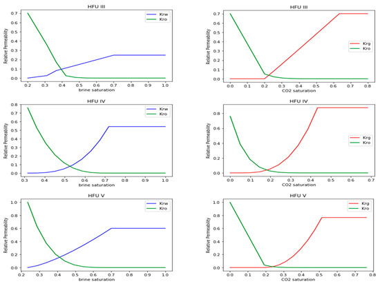
Figure 1.
Relative permeability curves of water(brine)-oil (left) and gas (CO2)-oil (right) created as a function of HFU of the Farnsworth Field Unit. HFU III-V were considered for both water-oil and oil-gas relative permeability curves. HFU III-V represents intermediate to highest permeability of Morrow B sandstone at a given porosity.
2.2. Parametric Method
The parametric method is an analytical procedure that uses common statistical information such as mean (mj) and standard deviation (sj) and easily quantifies uncertainty. The mathematical procedures are illustrated in Equations (6)–(11). The first step in parametric uncertainty quantification is to transform the mean (mj) and standard deviation (sj) from the original space to the lognormal mean (αj) and lognormal standard deviation (βj) as shown in Equations (7) and (8), respectively. The output lognormal mean (αΩ) and lognormal variance (βΩ2) of hydrocarbon initially in place (HCIIP) is computed by summing input lognormal mean (αj) and lognormal variance (βj2) 8s illustrated in Equations (8) and (9), respectively. Equation (14) is used to compute the relative impact of individual input. A flow chart illustrating the parametric method is shown in Figure 2.
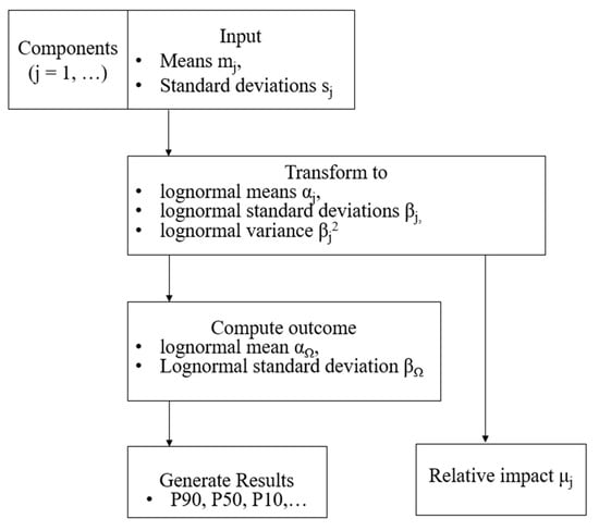
Figure 2.
A flow chart showing a parametric procedure in probabilistic reserves estimation.
A lognormal output of mean (αΩ) and standard deviation (βΩ) are used to generate various statistical measurements. These statistical outputs are categorized into three main divisions that include measures of location, measures of variability, and measures of shape. For example, P90, P50, P10, variance, and P10-to-P90 ratio are shown in Equations (12)–(16), respectively [24].
2.3. Plotting Tools
In this work, two approaches were utilized to present the probabilistic distribution (expectation plots) of HCIIP estimation. They were the “manual” approach and the Microsoft Excel built-in function. The manual approach is generated with Equation (17). The in the equation can be interpreted as the number of lognormal standard deviations. It is obvious from the equation that one needs only the lognormal mean (α) and lognormal standard deviation (β). The expectation curve becomes the exceedance probabilities (at various confidence levels) vs. Pc (GCO2).
Microsoft Excel has two built-in functions that can be utilized to generate expectation curves (e.g., GCO2) at various confidence levels. These are LOGNORM.INV (x, lognormal mean, lognormal standard deviation) and LOGNORM.INV (p, lognormal mean, lognormal standard deviation). All input variables (x, α, β) > 0. The “p” is classified as a cumulative probability (0 ≤ p ≤ 1). A plot of exceedance probabilities (1 − p) vs. x is the expectation curve from these two functions. Outcomes from parametric studies can also be illustrated by using a “log probability plot”. This straight-line plot elaborates the relationships between key confidence levels.
3. Farnsworth Field Unit Static Model
The SWP has developed several generational geological models over the years, revolving around the acquisition of a new dataset. Ampomah et al. [25] presented the second-generation geological model, which was based on preliminary seismic interpretations. In this work, reservoir properties such as porosity and permeability distributions were modeled with geostatistical methods using data from core and well logs. In 2016, Ampomah et al. [26] presented an improved geological model that modeled the field permeability distribution by developing correlations that separated the east and west sides of the field, which appear to have different behaviors. Detailed geological descriptions for FWU have been presented in several publications [1,25,26,27,28,29,30,31,32]. Ross-Coss et al. [33] presented an updated geological model for the SWP project, which significantly improved the site characterization efforts at FWU. This work developed a hydraulic flow unit (HFU) workflow based on pore throat aperture. The approach delineated the target reservoir into eight geological units. The analysis showed that diagenetic processes highly influenced reservoir property distribution as compared to depositional processes. The HFU methodology has been the basis for subsequent model improvements within the Morrow B Sand at FWU.
Balch et al. [34] presented the latest static model, which forms the basis for this work. This model extends from the vertical extent of the model to units above and below the reservoir and cap rock. There are 14 geologic horizons. The improved static model has a grid distribution of 189 × 179 × 106 with a total 3D grid of 3.6 million cells. Each grid block has a dimension of 100 × 100 ft. Figure 3 shows the geological zones used for the structural framework. This model does not include any previously mapped faults as ongoing work has thrown existence of such faults into doubt. Reservoir properties for this latest static model have been mapped from the Thirteen Finger Limestone (one of the caprocks) to the base of the Morrow B sandstone. The property modeling workflow applied to each formation depended on the data available and the formation characteristics. Integration methods included artificial neural network facies identification from well logs and cores, spatial variogram analysis, discrete and continuous distributions, and co-simulation with elastic inversion properties. Spatial variograms from 3D seismic acoustic impedance were used to condition property modeling within the upper layers due to limited well-log information. The prominent caprock layers within this upper section include the Thirteen Finger Limestone and Morrow Shale.
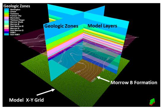
Figure 3.
Geologic model framework elements.
The Morrow B formation was the target reservoir; it ranges in depth from 7550 ft to 7950 ft with an average dip of less than one degree. It has been interpreted as a fluvial incised-valley deposit [29,30]. The thickness maps were used to estimate formation volume and architecture. The Morrow B has an average thickness of 22 ft on the west side of the field and 52 ft thick on the east side, with a mean thickness for the field of 24.47 ft and a standard deviation of 11.7 ft [33]. Figure 4 shows the net thickness map for FWU within the field unit boundary. The thickest sands are restricted to the middle of the field, whereas the sands thin along the periphery. Thicker accumulations occur in discreet areas such as to the west of well 13-10A and to the east of well 32-8. The established HFU methodology based on the Winland R35 was used to model porosity and permeability distribution within the Morrow B Sand. Fifty-one wells with core porosity and permeability were utilized in the HFU workflow, which quantified the heterogeneity within the target zone resulting in eight (8) distinct delineations.
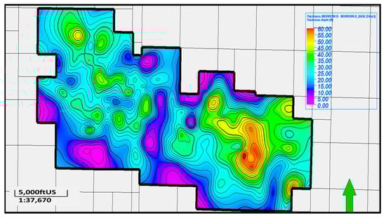
Figure 4.
Net sand thickness within Morrow B reservoir based on well top information. The mean of the net sand is 24.47 ft with a standard deviation of 11.65 ft.
Figure 5 illustrates how the depth and GR log for well 13-10A correspond to bedding and core description. Subsequent columns illustrate log, core, and thin section porosity along with log and core permeability. Porosity and permeability values were used to compute the LogR35 log. Thin section mineralogy and pore type summation columns were created based on point count data. Type thin sections for HFU1, HFU3, and HFU8 were placed in relative order to display where within the reservoir those particular HFUs were located, and a depiction of the pore type associated with that HFU. Thin Section 1 in Figure 5 is representative of HFU3. Here, intergranular space is almost filled with siderite cement and detrital clay. However, there is a large amount of intragranular macroporosity associated with grain dissolution. This hydraulic unit’s relatively high value for porosity does not correspond to a high permeability value because of the lower likelihood of intragranular space creating interconnected networks. From the thin section derived mineralogy and porosity classes, it becomes apparent that the degree of cementation and the degree of intergranular porosity development are primary controls on porosity and permeability. Figure 6 shows a plot of porosity and log permeability to depict the delineation within the reservoir based on the HFU. Figure 7 shows the 3D distribution of porosity of the target Morrow B reservoir. Figure 8 shows modeled permeability based on the porosity–permeability relationship.
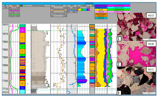
Figure 5.
Well section displaying reservoir interval for well 13-10A on west side of field. From left to right columns are depth (MD), gamma, bedding, sedimentary features, core description, porosity, permeability, LogR35, HFU categories, thin section derived mineralogy, thin section pore type, and thin section photos displaying scale bar and HFU (designated HU in this figure). Number on thin section image corresponds to location in core. Pink coloration in thin sections is pink-dyed epoxy in pore space.
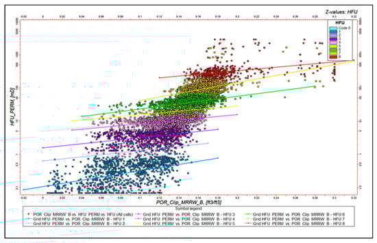
Figure 6.
Porosity versus permeability for the 51 cored wells, separated by pore throat size into hydraulic flow units.
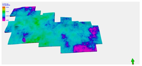
Figure 7.
Porosity distribution for top of Morrow B created using Gaussian random function simulation co-kriged using the volumes computed from the HFU property.
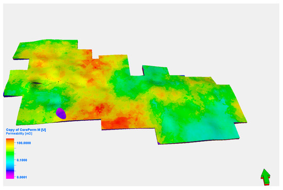
Figure 8.
Permeability distribution created by propagating permeability as a function of porosity defined by hydraulic units. Defining permeability in this way ensured that trends followed those predicted by the HFUs and did not simply assign high permeability values to high porosity values.
Volumetric Analysis
Initial fluid saturations for FWU were measured from special core analysis. The mean of oil saturation was 69%, with a standard deviation of 3.45%. The initial reservoir pressure and the temperature were 2217.7 psia at a datum of 4900 ft subsea and 168°F, respectively. The original bubble point pressure was 2073.7 psia, and a miscibility mean pressure range of about 4200–4500 psia was also observed. The reservoir was slightly undersaturated at the time of discovery. The supercritical CO2 (ScCO2) density was calculated using the Span and Wagner equation of state [35]. The mean and standard deviation of the ScCO2 was estimated to be 47.7 lbm/ft3 and 0.47 lbm/ft3, respectively. Based on the relative permeability curve of the FWU in conjunction with Equation (5), the mean efficiency factor was 69.9%, with a standard deviation of 22.6%.
The several volumetric reserves’ computational parameters mentioned in the above paragraphs, including area, net thickness, porosity, fluid saturation, ScCO2 density, and storage efficiency factor, were used in analyzing the uncertainty of storage capacity potential for the Morrow B reservoir using the parametric methods. A summary of input parameters is presented in Table 1. All input parameters were assumed to be lognormal distributed, although porosity, saturation, and ScCO2 density depicted close to normal distribution due to their minute standard deviations, and these are illustrated in Figure 9.

Table 1.
Mean and standard deviation of the input parameters used for the analysis.
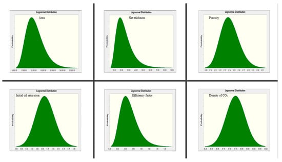
Figure 9.
The probability density function distribution of the input parameters generated by the Monte Carlo simulation.
4. Results and Discussion
The main objective was to quantify the storage capacity of CO2 in the Farnsworth Field Unit using the parametric method and to analyze the contribution of uncertainties of the input parameters to the total uncertainty. The Monte Carlo simulation was also presented to validate the results generated by the parametric method. This paper included the presentation of a new static model of the field and presented a different methodology in the estimation storage efficiency factor.
Most studies and simulations of the FWU have been focused on the west side of the field, since this is the part of the field where the CO EOR project has been conducted. The new model presented in this paper examines the CO2 storage capacity of both the west and east sides of the FWU, as the east side may eventually have interest for CO2 EOR or carbon storage. In 2010, the average pressure recorded on the east side was about 4700 psia [27]. The high pressure was a result of a successful waterflood and significantly demonstrates that minimum miscibility pressure could be achieved if CO2 is injected into this side of the field.
Figure 9 shows the distribution of the input parameters of the FWU. Distribution in nature was assumed to follow the logarithmic distribution. When the deviation of a group of variables is small, the values are closer to each other. Then, the distribution of the variables in the group is normal. However, when the deviation of the variables is large, that is, the values are farther from each other, then the distribution of the variables in the group is skewed. Now, from the outputted distribution of the input parameters, the porosity and the initial oil saturation were normally distributed, but the area, net thickness, and efficiency factor were highly dispersed, which further confirms the high heterogeneity of the formation.
The storage efficiency factor is one of the most uncertain parameters using the volumetric approach in estimating the storage capacity of a geologic formation. It is influenced by both rock and fluid properties. Studies show that the FWU is highly heterogeneous [19,27], and also, due to the alternating water and gas injection, the wettability of the Morrow B reservoir has changed to intermediate wet or mixed wet [19]. The estimation of the storage efficiency factor using the relative permeability curve as a function of HFU better represents the changes that have taken place in the reservoir due to productivity-enhancing techniques. HFUs III-V were considered in the estimation of the storage efficiency factor, as these represent the intermediate to highest permeability of the Morrow B sandstone at a given porosity (Figure 9). The relative permeability generated from these core samples was measured at an increasing order of pressure values from 3000 psi to 4000 psi, which mimics the miscibility pressure of the reservoir. From Equation (5), the denominator represents the theoretical space available for CO2 while the numerator represents the actual space available for CO2. Assuming a constant irreducible water saturation (Swc), the storage efficiency factor increases with reducing irreducible oil saturation after CO2 injection (Sorg) and critical gas saturation (Sgr).
The volumetric approach suggested by the USDOE [8] for oil and gas depleted reservoirs was altered and used to estimate the storage capacity of the Morrow B reservoir. The volumetric analysis uses reservoir rock and reservoir fluid properties to calculate hydrocarbon initially in place and the portion that can be recovered. Estimations of reserves using this approach always result in uncertainties with the output. Based on the degree of uncertainty, reserves are classified as proven (1P or P90), probable (2P or P50), and possible (3P or P10) [36]. As a result, the probabilistic approach was used, which gives details of the entire range of possible outcomes of the estimates instead of a single value like the deterministic approach. Below is a statistical measure illustrating the quantities of the storage capacity of the supercritical CO2 (GCO2) in the Farnsworth Unit (Morrow B reservoir).
From Table 2, P90 of both the parametric and the Monte Carlo simulation methods yielded about 8 MMtons, indicating a 90% probability that the estimated GCO2 will be at least 8 MMtons or 10% confidence that the estimated GCO2 will be less than 8 MMtons. The P50, which equals about 18 MMtons, is the best estimate in terms of the probabilistic approach, and it signifies a 50% probability that the estimated GCO2 will be at least 18 MMtons. The P10 is the most unlikely estimate in comparison to the P90 and P50. The P10 for both methods is about 41 MMtons, and it shows a 90% probability that the GCO2 will be less than 41 MMtons. The deterministic value is computed as the mean, which is about 22 MMtons for both methods. There is a 37.6% probability that at least the estimated GCO2 will be equal to the deterministic value.
Table 2.
Summary of the statistical measure of the storage capacity distribution.
Figure 10 shows the expectation curve, which illustrates the probabilistic distribution of the CO2 storage estimation of the Morrow B reservoir. The expectation curve shows the outcome of the estimated storage capacity at different confidence levels. The P99 and P1 on the expectation curve can serve as a good practical boundary for estimating the storage capacity of the Morrow B sandstone. The expectation curve of both the parametric and the Monte Carlo simulation yielded practically the same results. However, 10,000 simulation runs were needed for the Monte Carlo simulation to generate these outputs. Also, for the Monte Carlo simulation, prior knowledge of the results should be known to serve as a guide for the number of simulations runs. Most of the time, the mean value is used. From the expectation curve, it can be deduced that the probability that the GCO2 will lie between 7.81 and 40.52 MMtons is 80%.
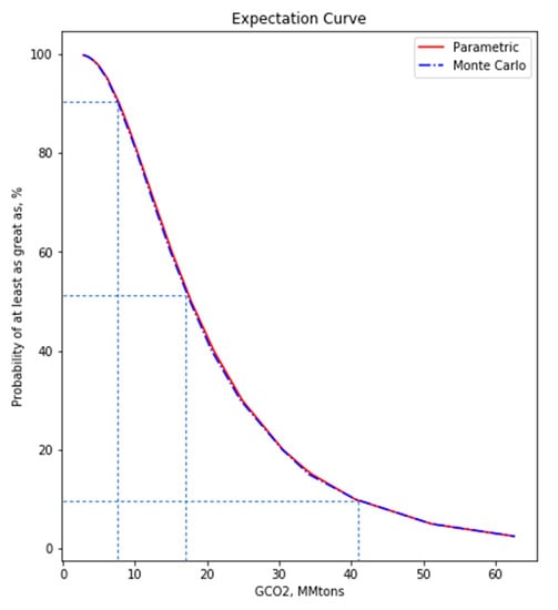
Figure 10.
Expectation curve illustrating the CO2 storage capacity at a different confidence level.
Figure 11 illustrates a log probability plot (P90-P50-P10 straight line). From the log probability plot, P90, P50, and P10 correspond to −1.2816, 0, and 1.2816 on the number of lognormal standard deviations axis, respectively. Hence, in terms of the probability distribution, it is in reverse order to the expectation curve. That is, the P90 comes first, followed by the P50, then the P10 in ascending order. This P90-P50-P10 straight line is similar to the expectation curve because all other statistical measures can be found on this straight line. Hence, the P90-P50-P10 straight line displays the entire range of the estimated distribution.
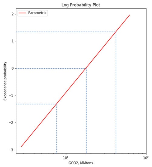
Figure 11.
Log probability plot showing the probabilistic distribution of the storage capacity of the Morrow B reservoir.
The standard deviation allocated to each of the input parameters indicates the uncertainty with the mean value. The degree of the uncertainty value stems from how difficult it is to determine that parameter. For instance, from Table 1, the standard deviation of the net thickness is about half of its mean value, which signifies how uncertain and difficult it is to accurately determine the exact value. However, the standard deviation of the ScCO2 density is insignificant as compared to its mean value. This is valid because the mean value is established using different sophisticated pressure equipment in reading the miscibility pressure through repeated experiments. These are also observed from Figure 9; the net thickness is positively skewed while the ScCO2 density seems symmetrical.
From the expectation curve, the mean ≠ median ≠ mode and signifies the skewness of the output probability density function. The expectation curve provides a good way of visualizing the total uncertainty. The narrower the curve or the closer the curve is to the vertical axis, the less is the total uncertainty. The log probability plot (P90-P50-P10 straight line) also provides a way of analyzing the uncertainty. The steeper the P90-P50-P10 straight line, the lesser the uncertainty to the total outcome.
The overall uncertainty of the Morrow B has a coefficient of variation of 71%, which translated into a standard deviation of about 16 MMtons. The total uncertainty of output increases with the product of input parameters. Hence, the total uncertainty is a result of the degree of uncertainty of the individual input parameters. A relative impact plot was constructed to analyze the uncertainty of the individual input parameters towards the total uncertainty.
From the relative impact plot showing in Figure 12 and Figure 13, the net thickness contributed the most to the total uncertainty of about 50%, followed by the efficiency factor, which contributed about 25% to the total uncertainty for both the parametric and Monte Carlo simulation. The net thickness, efficiency factor, and area together contributed about 95% to the total uncertainty. Relatively, the contribution of the efficiency factor to the total uncertainty was less considering the different parameters which affect it. However, this was expected considering how long the FWU has been produced; there were enough data to estimate the efficiency factor.
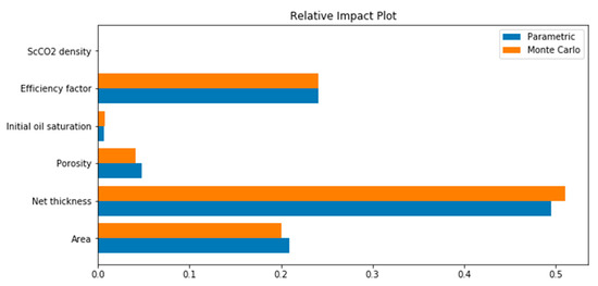
Figure 12.
Relative impact plot illustrating the contribution of the input parameters to the total uncertainty. This plot also compares the sensitivity analysis of both the parametric method and the Monte Carlo simulation.
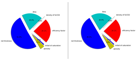
Figure 13.
Pie chart showcasing impact of the input parameters to the total uncertainty in percentages. The left and right charts represent the results generated by the Monte Carlo simulation and the parametric method, respectively.
5. Concluding Remarks
This work utilized an approach using the relative permeability curve as a function of the hydrologic flow unit to determine the storage efficiency factor and employed the parametric method to estimate the storage capacity of the Morrow B reservoir. It also shows sensitivity analysis of the input parameters towards the total uncertainty.
From the new static model presented in this paper, it appears that the eastern side of the field has sufficient storage capacity to make CCUS a feasible proposition, given the right economic conditions.
The use of relative permeability curves to estimate storage efficiency factors is an effective and feasible approach. It is concluded that for constant irreducible water saturation, the storage efficiency factor increases with the reduction of irreducible oil saturation after CO2 injection (Sorg) and critical gas saturation (Sgc).
From the probabilistic output generated by both techniques, the parametric method results show that at least 7.81 MMtons can be stored, 17.79 MMtons of CO2 can probably be stored, and it may be possible to store as much as 40.52 MMtons of CO2 in the Morrow B reservoir. The results outputted by the Monte Carlo simulation show similar results; 7.68 MMtons is at least proven to be stored, 17.63 MMtons can probably be stored, and it may be possible to store as much as 40.58 MMtons of CO2 in the Morrow B reservoir. The deterministic value, which is the single best estimate, was determined from the parametric method and Monte Carlo simulation to be 21.87 and 21.63 MMtons, respectively. From the relative impact plot, the net thickness, storage efficiency factor, and area contributed about 95% to the total uncertainty for both techniques. To significantly improve the estimation of the storage capacity of the Morrow B reservoir, this percentage needs to be reduced drastically. The net thickness contributed the most to the total uncertainty, and this should be the top-most priority to reduce the total uncertainty and better estimate the storage capacity.
The probabilistic approach (parametric method) was successfully used to estimate the storage capacity. Comparing both the parametric method and the Monte Carlo simulation, the results were practically the same, although 10,000 simulation runs were used, and this illustrates how computationally expensive the Monte Carlo simulation is. The parametric method assumes input variables to be lognormally distributed. It is an analytical procedure and can be performed in a simple spreadsheet application. This technique can be applied in all disciplines that seek to quantify the feasibility of a project while analyzing and quantifying total uncertainty. This technique may also assist management in decision-making procedures by helping them to arrive at a viable conclusion.
Author Contributions
Conceptualization, W.A.; methodology, W.A., J.A. and D.R.-C.; software, J.A. and W.A.; validation, R.B., M.C. and D.R.-C.; formal analysis, J.A., W.A. and D.R.-C.; writing—original draft preparation, J.A., W.A. and D.R.-C.; writing—review and editing, M.C. and R.B.; visualization, J.A., W.A. and D.R.-C.; supervision, W.A.; funding acquisition, R.B. All authors have read and agreed to the published version of the manuscript.
Funding
Funding for this project was provided by the U.S. Department of Energy’s (DOE) National Energy Technology Laboratory (NETL) through the Southwest Regional Partnership on Carbon Sequestration (SWP) under Award No. DE-FC26-05NT42591.
Institutional Review Board Statement
Not applicable.
Informed Consent Statement
Not applicable.
Data Availability Statement
Not applicable.
Conflicts of Interest
The authors declare no conflict of interest.
References
- Morgan, A.; Grigg, R.; Ampomah, W. A Gate-to-Gate Life Cycle Assessment for the CO2-EOR Operations at Farnsworth Unit (FWU). Energies 2021, 14, 2499. [Google Scholar] [CrossRef]
- Ruttinger, A.W.; Kannangara, M.; Shadbahr, J.; De Luna, P.; Bensebaa, F. How CO2-to-Diesel Technology Could Help Reach Net-Zero Emissions Targets: A Canadian Case Study. Energies 2021, 14, 6957. [Google Scholar] [CrossRef]
- García-Mariaca, A.; Llera-Sastresa, E. Review on Carbon Capture in ICE Driven Transport. Energies 2021, 14, 6865. [Google Scholar] [CrossRef]
- Shreyash, N.; Sonker, M.; Bajpai, S.; Tiwary, S.K.; Khan, M.A.; Raj, S.; Sharma, T.; Biswas, S. The Review of Carbon Capture-Storage Technologies and Developing Fuel Cells for Enhancing Utilization. Energies 2021, 14, 4978. [Google Scholar] [CrossRef]
- Pingping, S.; Xinwei, L.; Qiujie, L. Methodology for estimation of CO2 storage capacity in reservoirs. Pet. Explor. Dev. 2009, 36, 216–220. [Google Scholar] [CrossRef]
- Bachu, S.; Bonijoly, D.; Bradshaw, J.; Burruss, R.; Holloway, S.; Christensen, N.P.; Mathiassen, O.M. CO2 storage capacity estimation: Methodology and gaps. Int. J. Greenh. Gas Control 2007, 1, 430–443. [Google Scholar] [CrossRef] [Green Version]
- Goodman, A.; Hakala, A.; Bromhal, G.; Deel, D.; Rodosta, T.; Frailey, S.; Small, M.; Allen, D.; Romanov, V.; Fazio, J.; et al. U.S. DOE methodology for the development of geologic storage potential for carbon dioxide at the national and regional scale. Int. J. Greenh. Gas Control 2011, 5, 952–965. [Google Scholar] [CrossRef]
- Hall, G. The US 2012 Carbon Utilization and Storage Atlas; US Department of Energy: Washington, DC, USA, 2012; p. 130.
- IPCC. IPCC Special Report: Carbon Dioxide Capture and Storage. CMAJ 2004, 171, 1327. [Google Scholar] [CrossRef]
- Rossi, F.; Gambelli, A.M. Thermodynamic phase equilibrium of single-guest hydrate and formation data of hydrate in presence of chemical additives: A review. Fluid Phase Equilibria 2021, 536, 112958. [Google Scholar] [CrossRef]
- Frailey, S.M. Methods for estimating CO2 storage in saline reservoirs. Energy Procedia 2009, 1, 2769–2776. [Google Scholar] [CrossRef] [Green Version]
- Levine, J.S.; Fukai, I.; Soeder, D.; Bromhal, G.; Dilmore, R.M.; Guthrie, G.D.; Rodosta, T.; Sanguinito, S.; Frailey, S.; Gorecki, C.; et al. U.S. DOE NETL methodology for estimating the prospective CO2 storage resource of shales at the national and regional scale. Int. J. Greenh. Gas Control 2016, 51, 81–94. [Google Scholar] [CrossRef] [Green Version]
- Pyrcz, M.J.; White, C.D. Uncertainty in reservoir modeling. Interpretation 2015, 3, SQ7–SQ19. [Google Scholar] [CrossRef]
- Ma, Y.Z.; La Pointe, P.R. Uncertainty Analysis in Reservoir Characterization and Management: How much should we know about what we don’t know? AAPG Memoir 2011, 96, 1–15. [Google Scholar] [CrossRef]
- Ziegel, E.R.; Deutsch, C.V.; Journel, A.G. Geostatistical Software Library and User’s Guide. Technometrics 1998, 40, 357. [Google Scholar] [CrossRef] [Green Version]
- Bachu, S. Review of CO2 storage efficiency in deep saline aquifers. Int. J. Greenh. Gas Control. 2015, 40, 188–202. [Google Scholar] [CrossRef]
- Brennan, S.T. The U.S. Geological Survey carbon dioxide storage efficiency value methodology: Results and observations. Energy Procedia 2014, 63, 5123–5129. [Google Scholar] [CrossRef] [Green Version]
- Park, J.; Yang, M.; Kim, S.; Lee, M.; Wang, S. Estimates of scCO2 Storage and Sealing Capacity of the Janggi Basin in Korea Based on Laboratory Scale Experiments. Minerals 2019, 9, 515. [Google Scholar] [CrossRef] [Green Version]
- Rasmussen, L.; Fan, T.; Rinehart, A.; Luhmann, A.; Ampomah, W.; Dewers, T.; Heath, J.; Cather, M.; Grigg, R. Carbon Storage and Enhanced Oil Recovery in Pennsylvanian Morrow Formation Clastic Reservoirs: Controls on Oil–Brine and Oil–CO2 Relative Permeability from Diagenetic Heterogeneity and Evolving Wettability. Energies 2019, 12, 3663. [Google Scholar] [CrossRef] [Green Version]
- Ampomah, W.; Balch, R.S.; Chen, H.-Y.; Gunda, D.; Cather, M. Probabilistic reserves assessment and evaluation of sandstone reservoir in the Anadarko Basin. In Proceedings of the SPE/IAEE Hydrocarbon Economics and Evaluation Symposium, Houston, TX, USA, 17–18 May 2016; Volume 16. [Google Scholar] [CrossRef]
- Cronquist, C. Estimation and Classification of Reserves of Crude Oil, Natural Gas and Condensate; Society of Petroleum Engineers: Richardson, TX, USA, 2001. [Google Scholar]
- Chen, H.-Y. Engineering Reservoir Mechanics. Ph.D. Thesis, New Mexico Tech, Socorro, NM, USA, 2012. [Google Scholar]
- Morgan, J.; Gordon, D. Influence of Pore Geometry on Water-Oil Relative Permeability. J. Pet. Technol. 1970, 22, 1199–1208. [Google Scholar] [CrossRef]
- Capen, E.C. Probabilistic reserves! Here at last? SPE Reserv. Eval. Eng. 2001, 4, 387–394. [Google Scholar] [CrossRef]
- Ampomah, W.; Balch, R.S.; Grigg, R.B. Analysis of Upscaling Algorithms in Heterogeneous Reservoirs with Different Recovery Processes. In Proceedings of the SPE Production and Operations Symposium, Oklahoma City, OK, USA, 1–5 March 2015. [Google Scholar]
- Ampomah, W.; Balch, R.S.; Ross-Coss, D.; Hutton, A.; Cather, M.; Will, R.A. An Integrated Approach for Characterizing a Sandstone Reservoir in the Anadarko Basin. In Proceedings of the Offshore Technology Conference, Houston, TX, USA, 2–5 May 2016. [Google Scholar]
- Ampomah, W.; Balch, R.S.; Grigg, R.B.; Will, R.; Dai, Z.; White, M.D. Farnsworth Field CO2-EOR Project: Performance Case History. In Proceedings of the SPE Improved Oil Recovery Conference, Tulsa, OK, USA, 11 April 2016. OnePetro. [Google Scholar]
- Ampomah, W.; Balch, R.S.; Grigg, R.B.; Dai, Z.; Pan, F. Compositional Simulation of CO2 Storage Capacity in Depleted Oil Reservoirs. In Proceedings of the Carbon Management Technology Conference, Sugar Land, TX, USA, 17–19 November 2015. [Google Scholar]
- Hutton, A.C. Geophysical Modeling and Structural Interpretation of a 3D Reflection Seismic Survey in Farnsworth Unit, TX. Master’s Thesis, New Mexico Institute of Mining and Technology, Socorro, NM, USA, 2015. [Google Scholar]
- Gallagher, S.R. Depositional and Diagenetic Controls on Reservoir Heterogeneity: Upper Morrow Sandstone, Farnsworth Unit, Ochiltree County, Texas. Ph.D. Thesis, New Mexico Institute of Mining and Technology, Socorro, NM, USA, 2014. [Google Scholar]
- Czoski, P. Geologic Characterization of the Morrow B Reservoir in Farnsworth Unit, TX Using 3D VSP Seismic, Seismic Attributes, and Well Logs. Master’s Thesis, New Mexico Institute of Mining and Technology, Socorro, NM, USA, 2014; p. 101. [Google Scholar]
- Munson, T.W. Depositional, diagenetic, and production history of the Upper Morrowan Buckhaults Sandstone, Farnsworth Field, Ochiltree County Texas. Shale Shak. Dig. 1994, 40, 2–20. [Google Scholar]
- Ross-Coss, D.; Ampomah, W.; Cather, M.; Balch, R.S.; Mozley, P.; Rasmussen, L. An Improved Approach for Sandstone Reservoir Characterization. In Proceedings of the SPE Western Regional Meeting, Anchorage, AL, USA, 23–26 May 2016. [Google Scholar]
- Balch, R.; McPherson, B.; Will, R.A.; Ampomah, W. Recent Developments in Modeling: Farnsworth Texas, CO 2 EOR Carbon Sequestration Project. In Proceedings of the 15th Greenhouse Gas Control Technologies Conference, Abu Dhabi, UAE, 15–18 March 2021; Volume 2. [Google Scholar]
- Span, R.; Wagner, W. A New Equation of State for Carbon Dioxide Covering the Fluid Region from the Triple-Point Temperature to 1100 K at Pressures up to 800 MPa. J. Phys. Chem. Ref. Data 1996, 25, 1509–1596. [Google Scholar] [CrossRef] [Green Version]
- Etherington, J.; Ritter, J. The 2007 SPE/WPC/AAPG/SPEE Petroleum Resources Management System (PRMS). J. Can. Pet. Technol. 2008, 47. [Google Scholar] [CrossRef]
Publisher’s Note: MDPI stays neutral with regard to jurisdictional claims in published maps and institutional affiliations. |
© 2021 by the authors. Licensee MDPI, Basel, Switzerland. This article is an open access article distributed under the terms and conditions of the Creative Commons Attribution (CC BY) license (https://creativecommons.org/licenses/by/4.0/).