Optimized Charge Controller Schedule in Hybrid Solar-Battery Farms for Peak Load Reduction

Abstract

The goal of this paper is to optimally combine day-ahead solar and demand forecasts for the optimal battery schedule of a hybrid solar and battery farm connected to a distribution station. The objective is to achieve the maximum daily peak load reduction and charge battery with maximum solar photovoltaic energy. The innovative part of the paper lies in the treatment for the errors in solar and demand forecasts to then optimize the battery scheduler. To test the effectiveness of the proposed methodology, it was applied in the data science challenge Presumed Open Data 2021. With the historical Numerical Weather Prediction (NWP) data, solar power plant generation and distribution-level demand data provided, the proposed methodology was tested for four different seasons. The evaluation metric used is the peak reduction score (defined in the paper), and our approach has improved this KPI from 82.84 to 89.83. The solution developed achieved a final place of 5th (out of 55 teams) in the challenge.

1. Introduction

The cost of battery storage technologies has rapidly declined in the past two decades, and this trend is projected to continue in the horizon to 2030 [1]. This decline has facilitated various applications by integrating batteries with electricity generation and distribution [2,3]. For example, solar and wind energy suppliers have used batteries for stabilizing the power output and reducing the deviations from the day-ahead schedule. Utilities have used batteries to store cheap energy during off-peak hours and dispatch it during peak hours, which is commonly referred to as peak shaving. The optimal siting of batteries has also been used to postpone or reduce the cost of grid infrastructure.

In this paper, we are interested in an application where a load serving entity (LSE) integrates a storage device for solar farms which is also connected to a distribution system. We are particularly focusing on the day-ahead scheduling of such a device, through which the LSE can minimize the daily net peak by using as much solar energy as possible. The problem of day-ahead scheduling is critical, as it is a requirement to participate in electricity markets. The goal is reducing the peak load, as prices are higher during those hours. Charging the battery with the maximum possible solar energy is important, as it is the cheapest source of energy. Additionally, some regulations, such as Massachusetts Clean Energy standards, provide renewable energy credits if the peak demand is satisfied through renewable energy.

To generate an optimal day-ahead charging schedule that achieves the desired objectives, we divide the problem into three steps, which are demand forecasting, solar forecasting and battery scheduler. In the demand forecasting step, we train a machine learning model on historical data and generate a demand forecast for the next day. Similarly, in the solar forecasting step we train another machine learning model and predict the solar output for the next day. In the next step, we propose a battery scheduler that can ingest the previously generated forecasts and output an optimal schedule.

In the next section, we review some of the most popular machine learning algorithms for demand forecasting and load forecasting. We also review some of the literature on the day-ahead scheduling of batteries facing an uncertainty in forecasts. In Section 3, we introduce our machine learning methodologies for demand and solar forecasting. We also introduce our battery scheduler that can accept both perfect forecasts and forecasts with errors. In Section 4, we apply our approach to a case study from a data science challenge and compare the effectiveness of the solutions with other solutions. In Section 5, we provide some discussion and conclusions.

2. Literature Review

There is a great deal of interest in forecasting energy-related time series, specifically regarding the generation of renewable energy sources, load forecasting, electricity price forecasting or gas consumption forecasting [4,5,6].

2.1. Demand Forecasting Review

Driven by the needs of the energy markets and grid operators, electric load forecasting or demand forecasting has been a key research area for decades. Over the years, a multitude of methods have been proposed to achieve accurate forecasts and reduce operational costs and difficulties. Different time series modeling approaches include statistical methods such as moving averages and autoregressive models and state and frequency space approaches like Kalman filters and Fourier analysis. Lately, machine learning and deep learning approaches have become dominant [7]. For a pivotal review of classical approaches, see [8], and a more recent review focusing on short-term load forecasting is in [9]. A load forecast combination study is presented in [10], where the author combined forecasts from several sister models to enhance the accuracy of point load forecasts. Moving beyond point forecasts, probabilistic load forecasts are gaining traction, and a technical review can be found in [11].

2.2. Solar Forecasting Review

The higher penetration of solar energy gives an ever-growing importance to increasingly accurate forecasting [12]. To capture the local circumstances and phenomena of each individual plant, Machine Learning (ML) provides a widely used solution [13,14]. These algorithms on the day-ahead market are trained on historical Numerical Weather Prediction data and other cyclical variables, where the target is the active power production at the point of common coupling. According to [15], an accuracy gain of around 30% is achievable for ML modeling as opposed to NWP-based physics prediction. For the purpose of the temporal interpolation of irradiance, as well as to make the data stationary, the clearsky-index (CSI) is used in [16,17].

2.3. Scheduling of Battery Review

Several day-ahead optimization models are designed to schedule battery in day-ahead electricity markets [18,19]. These models either maximize for revenue or minimize for deviation penalties. These models generally satisfy the constraints related to the operation of battery. To account for the uncertainties in day-ahead forecasts, previous studies designed a two-stage stochastic optimization problem with a day-ahead forecast and several real time scenarios [20]. Instead of using scenarios to consider uncertainty, Toubeau et al. consider distributions derived from historical reserve activations.

Previous approaches either require estimating historical error distributions in forecasts or generating several future scenarios. While such approaches can provide robust solutions, they may be hard to solve or have the additional burden of quantifying such uncertainties. We take a different approach, assigning weights to time periods to prioritize them for charging or discharging. We describe our approach for a scheduler with imperfect forecasts in Section 3.4.2.

3. Methodology

Our approach is to divide the problem into three subparts, as laid out in Figure 1:

• Demand forecasting problem
• Solar forecasting problem
• Battery optimization problem

The main contribution of the paper is the optimal battery scheduling under uncertainty. The electric demand and solar forecasting modules play an auxiliary role, and the requirement was to deliver reliable and accurate forecasts to minimize uncertainty in the inputs. This was achieved using industry standard machine learning methods and some clever modeling techniques of input and output combination to increase forecast robustness.

3.1. Machine Learning Approach

3.1.1. Random Forest

A random forest is an ensemble learning method that builds numerous decision trees on slightly different slices of the training data and outputs the mode or mean of the individual trees. The literature shows that random forests are robust and resilient to overfitting and generalize well to various machine learning problems. Furthermore, these models provide useful insights such as ranking input features based on their relative importance. Later, in Section 4, we developed random forest models with 1000 trees to forecast daily energy consumption.

3.1.2. Gradient Boosting Regression Trees

Gradient boosting is an ensemble method that combines weak learners for a higher model accuracy, as suggested by Friedman in 2001 [21]. The predictor generated in gradient boosting is a linear combination of weak learners, and here tree models are utilized for this purpose. A sequence of models is built iteratively, starting from a constant initial prediction $F_0$ (in a least squares regression task, the mean of the target variable), and with each tree built on the residuals of the previous tree. To avoid overfitting, there is a shrinkage parameter (also called learning rate), which controls how much each tree contributes to the final model; this effectively slows learning down, yielding a better performance at the expense of requiring more iterations.

The final prediction, $F_N$, is calculated as follows:

$$F_N\left(x\right)=F_0+{\displaystyle \sum }_{i=1}^N\mathsf{\nu }*h_{i\left(x\right)}{}_{ }$$

(1)

where:

-

N is the number of individual trees built,

-

$F_0$ is the initial prediction,

-

$F_i$ is the prediction at stage i,

-

h is the prediction of an individual tree learner,

-

ν ∈ (0, 1] is the shrinkage parameter to reduce the effect of an individual tree in the sequence.

The general idea is to compute a sequence of simple trees, where each successive tree is built for the prediction residuals of the preceding tree. Each new base-learner is chosen to be maximally correlated with the negative gradient of the loss function, associated with the whole ensemble. This way the subsequent stages will focus harder on fitting these examples, and the resulting predictor is a linear combination of weak learners.

Utilizing boosting has many beneficial properties; various risk functions are applicable, and an intrinsic variable selection is carried out, which also resolves multicollinearity issues and works well with a large number of features without overfitting.

3.1.3. Feed-Forward Neural Networks

Neural networks are widely used nowadays in problems such as image processing or audio signal recognition. A neural net is composed of layers of neurons and connections between them. In the simplest architecture of a regression type neural net, in a feed forwarded net, the neurons in the input layer represent the features utilized, whereas the output layer contains a single neuron that is the target variable. The process whereby such a net is trained is called backpropagation.

3.1.4. Combined Forecasts

Among various forecast combination methods, simple average is the easiest one to implement and usually outperforms many other complicated combination schemes [22]., Taking the simple average of the selected individual forecasts to obtain the combined forecasts is surprisingly effective considering its simplicity. Another approach is stacking, which utilizes the predictions of different models as features in a meta learner model.

3.1.5. Hyperparameter Tuning

For each of the ML models trained, there is a hyperparameter grid search implemented. The parameters to control are chosen on a time-series-based five-fold cross validation of the training set. The first grid is on a wide scale of values, to then explore precisely the surrounding of the optimal ones with a grid search.

3.2. Demand Forecasting

This paper presents a refined methodology based on the implementation during the competition. As a subcomponent of the battery scheduler, the objective of the demand forecasting is relatively simple: accurately predict the daily peak hour and provide accurate forecasts in the afternoon discharge period to reduce the uncertainty of the scheduler. Accuracy and robustness can be ensured through a number of steps taken in feature engineering, the selected modeling techniques, and through forecast combination.

The proposed demand models are built on top of datetime, holiday and weather features, as listed in

Table 1. Input features used in demand forecasting.

Input Type	Input Features
Weather features	Lagged weather features 1–3 h Rolling mean and rolling standard deviation on 3–48 h horizons Heating degree days and cooling degree days Temperature–datetime interaction variables
Datetime features	Hour of day, day of week, day of month, day of year, week of year, month of year, year
Holiday features	Holidays and days immediately before and after holidays are marked as special
Solar features	PV generation forecast

. Datetime features capture time-variant trends, and we propose to use sine- and cosine-transformed date attributes to reflect the diurnal and annual cycles of these features. The electric load is driven by human behaviour, and holidays can have a great impact on it. Local holidays can be extracted using external tools such as the Workalendar Python library. (Workalendar offers classes able to handle calendars, list legal/religious holidays and give working-day-related computation functions. See https://github.com/peopledoc/workalendar for more, accessed on 20 August 2021.)

Some researchers tackled the load forecasting problem by combining weather stations [23,24]. As an initial estimate of the temperature and irradiance, we simply propose to take an average over all available stations. These estimates can then be used to generate a number of moving average windows features, as shown in the table above. Since we are working with weather forecasts, moving windows can cover data points both in the past and future relative to the forecast time. Heating degree days (HDD) and cooling degree days (CDD) are measures of how cold/warm the temperature was on a given day or during a period of days [25] and capture the heat perception of humans. Although not critical for non-linear models, a selection of temperature–date interaction variables were used as features similarly to the Vanilla benchmark described in [26].

Throughout the globe, the installed capacity of rooftop solar grows every year. Since it is behind the meter, this installed PV capacity is presented as negative demand when it comes to actual power consumption. At a substation level, one can only gather aggregated net demand data, not the actual consumption, and therefore demand models will be intrinsically flawed. Lacking actual generation data for rooftop solar, our proposed approach is to use PV generation data from a nearby solar farm as a proxy for behind-the-meter generation. This is of course a rough estimation that has its limitations and neglects differences in capacity, orientation, panel geometries, technologies, etc.

To achieve robust results and highly accurate demand forecasts, we propose using tree-based ensemble models, such as Random Forests, specifically scikit-learn’s Extra Trees algorithm, and gradient boosting methods like LightGBM and XGBoost. Individual models can be ranked and selected based on test accuracy. However, instead of using a single forecasting model we propose taking the mean of individual model forecasts for increased accuracy.

Since our proposed battery scheduler only uses demand forecasts from the afternoon discharge period, the modeling step should be limited to considering the 3:30 P.M. to 9 P.M. period only. This means fewer training samples but also more fine-tuned and accurate models focusing on the actual period of interest.

3.3. Solar Forecasting

In cases when there is data available regarding the panel geometry, i.e., panel tilts, tracking technology, etc., it is possible to model the irradiance on the panel. This tilted irradiance would be proportional to the DC power production. On the other hand, in the absence of panel geometry data, with a large amount of data, it is possible to create well generalizable ML models that learn the patterns of site-specific phenomena.

In this paper, the steps of solar forecasting are tackled with ML-based modeling. The model feature set includes NWP data as well as other cyclical data. The steps of modeling are the following:

• There is an inherent bias of NWP forecasts, as the grid points of NWP data are usually not precisely on a solar plant. To overcome this bias, there was a linear-regression-based debias method developed for the GHI predictions, so that the closest grid points would be used to predict GHI measurements at the site.
• Then, this irradiance and the temperature were used as features for modeling the active power on the PV site.
• To capture the possible timewise degradation of solar modules [27], as well as to see any effect of seasonality, numerous cyclic features were utilized in the modeling.
• The final modeling was done with scikit-learn-based Linear modeling and Random Forest.

The error metric of testing of the solar forecasting had two components, although the final model selection was based on the latter. Apart from these, R2 and CVRMSE were also considered for the general fit.

-

First, the Mean Absolute Percentage Error was used. The physical meaning of this error metric is the average absolute percentage difference of the prediction from the ground truth.

-

Secondly, the normalized Mean Absolute Error was used for the basis of model selection. The basis of normalization is the maximum measured power. The physical meaning of this error metric is the percentage of how high the average absolute error is compared to the farm capacity.

3.4. Battery Scheduling

In this subsection, we describe battery schedulers that use the upcoming week’s forecasts (both solar and demand forecasts) and generate a week-ahead battery operational schedule. First, we describe how we would schedule assuming there are no errors in forecasts. Next, we describe the scheduler that accounts for errors in forecasts.

3.4.1. Scheduler with Perfect Forecasts

We are interested in a scheduler with perfect forecasts, as it accepts actual demand and solar output and provides us with the best schedule. Instead of actuals, if we input forecasts, it will generate a schedule without accounting for errors in them. This schedule can then be compared with other schedules generated from battery schedulers that consider errors in forecasts. The optimal schedule should satisfy all operational and technical constraints related to the operation of a battery. Operational constraints include the time periods during which the battery can be either charged, discharged or kept empty. Technical constraints include the capacity of the battery and charge/discharge rate. The energy balance for each period states that the net charge into the battery is equal to the change in the energy state of the battery. We ignored the roundtrip efficiency and the minimum desired state of the battery for simplicity purposes.

As stated previously, there are two main goals for the battery scheduler. First, charge the battery with as much solar energy as possible and, second, reduce the evening peak load. We want to charge the battery to its full capacity before peak hours begin. If we are unable to do so on any non-sunny day, the scheduler can determine the deficit amount to charge from the grid. However, the preference is always to charge from the solar output before charging from the grid. To achieve the second goal, we calculate the maximum daily net peak and minimize it in the objective function. Since both goals are not conflicting with each other, we can simply add those two in the objective function.

Here is the optimization model formulation for a scheduler with perfect forecasts. Please refer to

Table 2. Table of Notations.

Variables
$b_t$	The rate of charge or discharge for period t
$p_t$	Charge rate from solar for period t
$q_t$	Energy stored in the battery at beginning of period t
$r$	Minimum daily net load across peak hours
Constants
$S_t$	Day-ahead solar forecast for period t
$L_t$	Day-ahead load forecast for period t
$P_{S_t}=\frac{e^{S_t}}{{{\displaystyle \sum }}_{t\in \Omega }^{}{e}^{S_t}}$	Weights/Pseudo probabilities to calculate expected generation
$P_{L_t}=\frac{e^{L_t}}{{{\displaystyle \sum }}_{t\in {\Omega }^{\prime }}^{}{e}^{L_t}}$	Weights/Pseudo probabilities to calculate expected net demand
B	Deviation factor from average net demand
$D=\left(\frac{{{\displaystyle \sum }}_{t\in {\Omega }^{\prime }}^{}{L}_t-C*0.5}{11}\right)$	Forecasted net demand during peak hours

for a complete list of the notations used in the model. All variables are denoted in lower case and parameters/constants in upper case. Let Ω denote the set of peak periods and Ω’ denote the set of non-peak periods.

$$Min r-{\displaystyle \sum }_{t\in {\Omega }^{\prime }}{p}_t$$

(2)

Solar charging constraints:

Charging periods: non-peak periods

$$p_t\le S_t, t\in {\Omega }^{\prime }$$

(3)

$$p_t-b_t\le 0, t\in {\Omega }^{\prime }$$

(4)

$$0\le b_t\le D, t\in {\Omega }^{\prime }$$

(5)

$${\displaystyle \sum }_{t\in {\Omega }^{\prime }}{b}_t*0.5=C$$

(6)

Peak hours discharge constraints:

Applicable during peak periods

$$-D\le b_t\le 0, t\in \Omega$$

(7)

$$r\ge L_t+b_t, t\in \Omega$$

(8)

$${\displaystyle \sum }_{t\in \Omega }{b}_t*0.5=-C$$

(9)

Battery operational constraints and boundary conditions:

$$q_t-q_{t-1}-b_{t-1}*0.5=0, t\in \Omega \cup {\Omega }^{\prime }$$

(10)

$$q_0=0, q_T=0$$

(11)

$$0\le q_t\le C, t\in \Omega \cup {\Omega }^{\prime }$$

(12)

Equation (3) determines that the amount of solar charge into the battery is less than the actual or forecast ones. Equation (4) determines that the solar charge into the battery is less than the total charge into the battery. Equation (5) determines that the total charge into the battery is less than its maximum charge rate of the battery. Equation (6) ensures that the total energy across all charging hours is equal to the battery’s capacity. Equation (7) makes sure that the discharge rate is less than the maximum possible discharge rate. Equation (8) is a way of calculating the maximum daily net peak, and we minimized it in the objective function. Equation (9) makes sure that we discharge the battery fully in the peak hours. Equations (10)–(12) keep track of the energy balance and limit the amount of energy stored in the battery, which is less than the capacity and boundary conditions on the energy state of the battery.

3.4.2. Scheduler with Imperfect Forecasts

In this subsection, we present the scheduler that considers potential errors in forecasts.

Deviations in solar forecasts: To account for potential deviations in solar forecasts, we scale down the forecasts by multiplying the forecasts with the weights. Scaling down guarantees that we charge much less than the forecast. To estimate weights for the charging periods, we apply exponential normalization (also referred to as SoftMax function). We also limit the charge rate, as in several time periods. This guarantees that we charge much less during early morning, and we gradually increase the charge rate as we approach the afternoon.

Deviations in load forecasts: Like solar forecasts, we multiply the load forecasts with the weights. These weights are also estimated by applying the SoftMax function on load forecasts. Scaling down on load forecasts can prevent committing to large amounts of discharge in one period, as forecast predicted it to be a peak period. We also put in an additional constraint, which guarantees that the scheduled net load is flat across all hours. We allow for some deviations, which are proportional to their forecasts.

Consider there are total T time periods in a day. For each period, we need to determine the $b_t,$i.e., the charge/discharge rate. Our objective is to maximize the total solar energy used to charge the battery and minimize the daily net peak during peak hours.

$$Min r-{\displaystyle \sum }_{t\in {\Omega }^{\prime }}{p}_t$$

(13)

Solar charging constraints:

Charging periods: non-peak periods

$$p_t\le S_t*P_{S_t}, t\in \Omega$$

(14)

$$l\le b_t\le \left(U-0.01*\left(t-10\right)\right), t \in \Omega$$

(15)

$$p_t-b_t\le 0, t\in \Omega$$

(16)

$$0\le b_t\le D, t\in \Omega$$

(17)

$$0\le b_t\le S_t+B*P_S{}_t, t\in \Omega$$

(18)

$${\displaystyle \sum }_{t\in {\Omega }^{\prime }}{b}_t*0.5=C$$

(19)

Peak hours discharge constraints:

Applicable during peak periods

$$-D\le b_t\le 0, t\in \Omega$$

(20)

$$L_t+b_t=D-B\left(P_{L_t}-\left(\frac{1}{\left|\Omega \right|}\right)\right) t\in \Omega$$

(21)

$${\displaystyle \sum }_{t\in \Omega }{b}_t*0.5=-C$$

(22)

$$(L_t+b_t)*P_L{}_t\ge r, t\in \Omega$$

(23)

Battery operational constraints and boundary conditions:

$$q_t-q_{t-1}-b_{t-1}*0.5=0, t\in \Omega \cup {\Omega }^{\prime }$$

(24)

$$q_0=0, q_T=0$$

(25)

$$0\le q_t\le C, t\in \Omega \cup {\Omega }^{\prime }$$

(26)

Equation (15) determines the limits on the charge rate for different time periods in the day. Equation (18) determines the time periods to charge from the grid on a charge deficit day. Equation (21) determines that the net load for each period is equal to the forecasted net demand and allows for some deviation.

In the next section, we apply the methodology to a case study and discuss the results.

4. Case Study: PoD Data Science Challenge

4.1. Competition Background

Presumed Open Data Projects are organized by Energy Systems Catapult, a technology and innovation centre in the United Kingdom. The challenge in 2021 was organized by Western Power Distribution. In this year’s competition, 55 teams, 142 individuals out of 72 different organizations/institutions and 15 different countries participated. Our team participated and reached the 5th position by the end of the competition.

4.2. Input Sources and Data

The Presumed Open Data Project 2021 challenge was about a 6 MWh/2.5 MW battery that is connected to a primary distribution substation and a 5 MW solar farm named Newton Downs Solar Plant, in Devon, southwest England. The battery can be charged daily between midnight to 3:30 P.M. to its full capacity by either charging from the solar plant or from the grid. It can then be discharged completely during evening peak hours (3:30 P.M. to 9 P.M.). The goal of the exercise was to generate a week-ahead battery schedule to support the distribution network to:

• Maximize the daily evening peak reduction,
• Maximize the amount of daily solar photovoltaic energy charging.

The historical generation from the solar farm was provided. Irradiance data from nearby weather stations were also provided. A complete list of data along with their granularities, made available in the competition, is shown in

Table 3. Given data and their granularities, further comments.

Data Type	Granularity	Comments
Historical temperature and irradiance data; temperature and irradiance predictions for the upcoming round’s period	60 min	The data are from multiple grid points of a Numerical Weather Prediction model MERRA-2. The precise prediction cycles of these points were unknown but are assumed to be constant.
Historical demand data on the substation	30 min	No data about the upcoming round’s period.
Historical photovoltaic generation data of the 5 MW Newton Downs Solar Plant.	30 min	No data about the upcoming round’s period.

.

The datasets are publicly available at the Western Power Distribution Open Data Hub site upon login [28].

4.3. Challenge Rounds

Overall, the challenge consisted of one practice round (Round 0) and 4 actual competition rounds (Rounds 1, 2, 3 and 4) as seen in

Table 4. Historical and submission sets for each round.

Challenge Round:	Given Historical Dataset:	Submission Dataset:
0	3 November 2017–22 July 2018	23 July 2018–29 July 2018
1	3 November 2017–15 October 2018	16 October 2018–22 October 2018
2	3 November 2017–9 March 2019	10 March 2019–16 March 2019
3	3 November 2017–17 December 2019	18 December 2019–24 December 2019
4	3 November 2017–2 July 2020	3 July 2020–9 July 2020

. There was a week’s time between each round to improve the methodology and prepare the next round’s solution. The data provided at the start of each round of the challenge was described in Section 4.2.

Please note that in each round the NWP temperature and irradiance data were given for both the historical and submission time periods. However, the demand and photovoltaic generation data were only made available for the historical time period.

4.4. Evaluation Metric

The pairing of the battery with the solar farm was expected to provide two benefits. First, to shift the solar energy generated earlier in the day to evening peak hours with little solar energy production. Second, to reduce the peak by discharging the battery and reducing strain on the distribution system. Overall, it results in a flexible, less carbon-intensive, but more reliable grid operation. To this end, the battery schedule was evaluated on how much solar energy was used to charge the battery and achieve the peak reduction.

The precise evaluation formula was described in the following equations. For a single day, it was calculated as:

$$S_d=R_{d,peak}\left(p_{d,1}{C}_1+p_{d,2}{C}_2\right)$$

(27)

where:

-

$S_d$ is the peak reduction score for a particular day,

-

$R_{d, peak}$ is the percentage peak reduction during the evening period on day d (old peak–new peak)/old peak,

-

$p_{d,1}$, $p_{d,2}$ indicate the proportion of energy stored in the battery from solar energy and from the grid, respectively, on day d

-

$C_1$, $C_2$ are the given constants and weights for the solar and grid energy, respectively. These weights are based on the relatively lifetime Greenhouse Gas emission intensity of solar and electricity from the grid around the substation.

To get the final peak reduction score for a particular submission, the simple average was taken of each day’s peak reduction score. In the competition, this number was the basis of comparison between each submission, and the goal was to maximize this number. The overall score for the competition was the average score over all rounds

4.5. Battery Operational Constraints

In each round, the week-ahead schedule should satisfy several constraints set by the organizer [29]:

1.

The maximum charge and discharge of power is 2.5 MW.

$$-2.5 \mathrm{MW}=-D \le b_t \le D=2.5 \mathrm{MW}$$

(28)

2.

The battery cannot charge beyond its capacity, $q_t$ (in MWh)

$$0\le q_t \le C=6 \mathrm{MWh}$$

(29)

3.

The total charge in the battery at the next time step $q_{d, k+1}$ is related to how much is currently in the battery and how much is charged within the battery at time k, i.e.,

$$q_t-q_{t-1}-b_{t-1}*0.5=0$$

(30)

4.

Charging ($b_t \ge 0$) is only allowed from midnight to 3.30 P.M. (t = 1 to 31).

5.

Discharging ($b_t \le 0$) is only allowed from 3.30 P.M. to 9 P.M. t = 31 to 42.

6.

The battery must be empty after discharging, i.e., $q_{ t}=0$ for $t=43, \dots , 48$.

4.6. Results of the Proposed Methodology

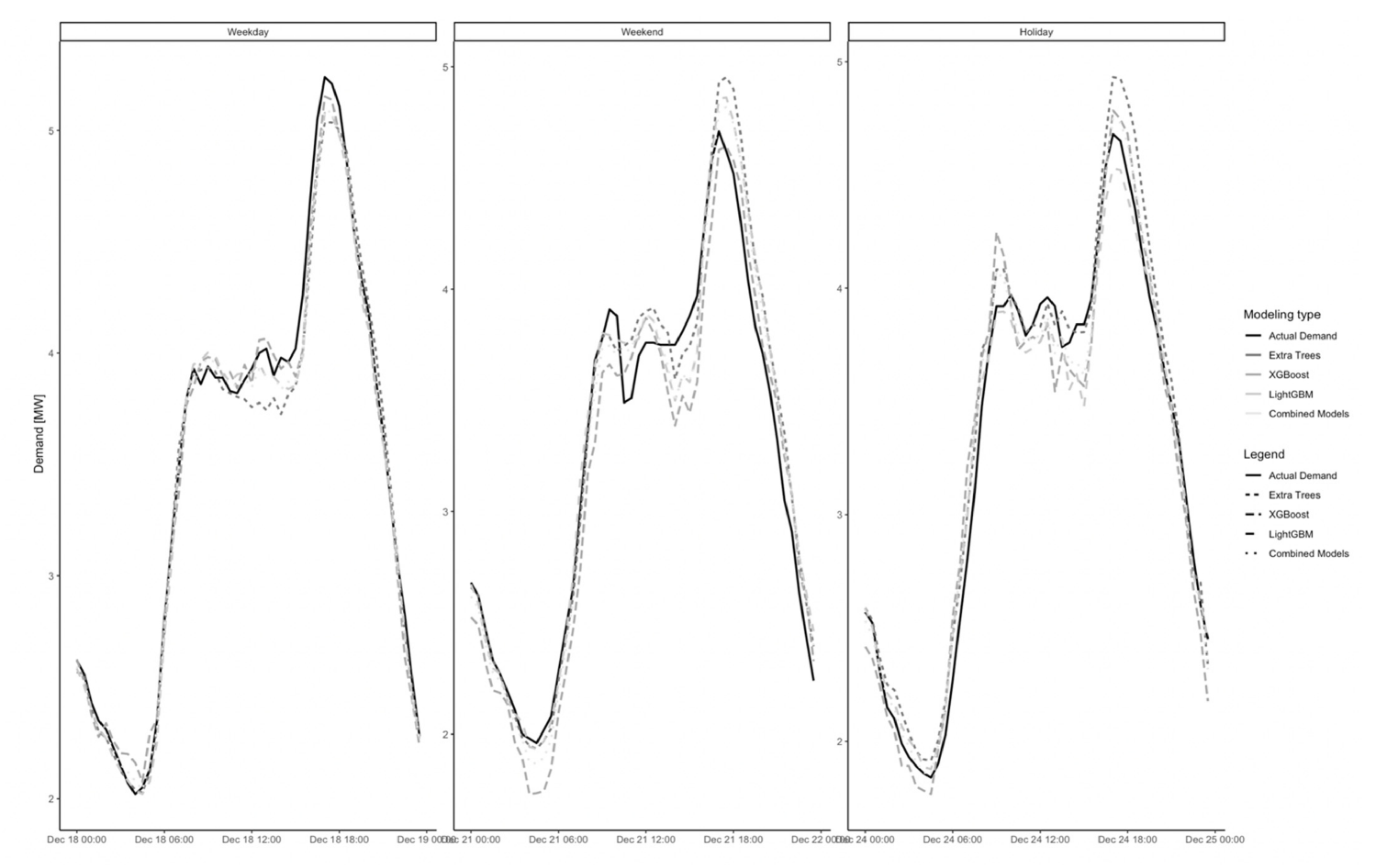
4.6.1. Demand Forecasting Results

Figure 2 and

Table 5. MAPE (%) values on the submission period for individual models and the combined result. Lowest error rate in bold, second lowest in italic.

Round	Extra Trees	XGBoost	LightGBM	Combined Forecast
1	4.531	8.301	5.347	5.292
2	2.965	4.704	3.371	3.359
3	5.419	4.501	4.042	4.522
4	5.637	5.731	4.864	5.330

summarizes the benefits of combining model forecasts through a simple averaging. On average, the model combination yields the MAPE of 4.626%, which is generally better than the individual model accuracy. While the performance of a single model could be quite volatile, the performance of the combination is relatively stable, achieving 2nd place in three out of four rounds. Throughout the rounds, both Extra Trees and LightGBM proved to be quite accurate. From a pure accuracy perspective, XGBoost seemed to lag behind, but still proved to bring useful information into the forecast combination. The measured accuracy of both the individual models and the combined forecast is generally in line with what has been reported in the demand forecasting literature (see [9] for comparison). The combined model’s goodness of fit was evaluated using R-square and CVRMSE metrics.

Table 6. R² and CVRMSE (%) values on the submission period for the combined result.

Round	R2	CVRMSE (%)
0	0.92	6.59
1	0.92	8.01
2	0.97	4.78
3	0.82	5.21
4	0.72	7.33

contains the results.

The proxy rooftop solar modeling approach was validated by adding the actual PV generation as an input for demand forecasting, which saw a substantial increase in model accuracy. In the competition setting, PV forecasts for the Newton Downs Solar Plant were used instead of PV generation actuals, which meant an extra dependency on the maturity and accuracy of the solar forecasting model but still offered increased accuracy.

4.6.2. Solar Forecasting Results

Table 7. Solar forecasting results for the 4 weeks of different test months.

Round	Test Month	Average CSI	UF	MAPE [%]	nMAE [%]	R2	CVRMSE
1	March	0.6	0.12	24.5	4.02	0.85	72.46
2	July	0.86	0.27	25.1	6.98	0.87	45.39
3	October	0.97	0.13	28.5	5.92	0.76	87.12
4	December	0.66	0.03	69.8	1.39	0.72	134.04

shows the month-by-month accuracies of the developed models, along with important aggregated influential factors:

◦

Average CSI stands for Clear Sky Index, indicating how clear a day is, on average, when compared to a modeled clearsky day. (Clearsky modeling has been performed with a default parameter set of the corresponding PVLIB modules.)

◦

UF stands for Utilization Factor, that is the overall real produced energy of the power plant as a percentage of the hypothetical case that the power plant was producing electricity on nominal capacity during the entire period.

The UF of the power plant ranges from 3% to 27%, being 3% in the winter period (December, round 4) and 27% in the summer period (July, round 2). The average CSI does not vary as highly as the UF. It ranges from 60% to 97% all year long, being the highest in the fall (October, round 3). Please note that where MAPE is the highest, the nMAE is the lowest and that is in round 4 (winter months). This is because production levels are very low, resulting in only 3% in UF. Please also note that the nMAE is the highest when the production levels are the highest, in the summer (July, round 2). Table 7 shows the R2 and CVRMSE results as well to show the fit of the model. Please note that CVRMSE results are particularly high due to nighttime 0 values that decrease the mean of the active power production. These results are on a par with the state-of-the-art research on solar forecasting [13,14].

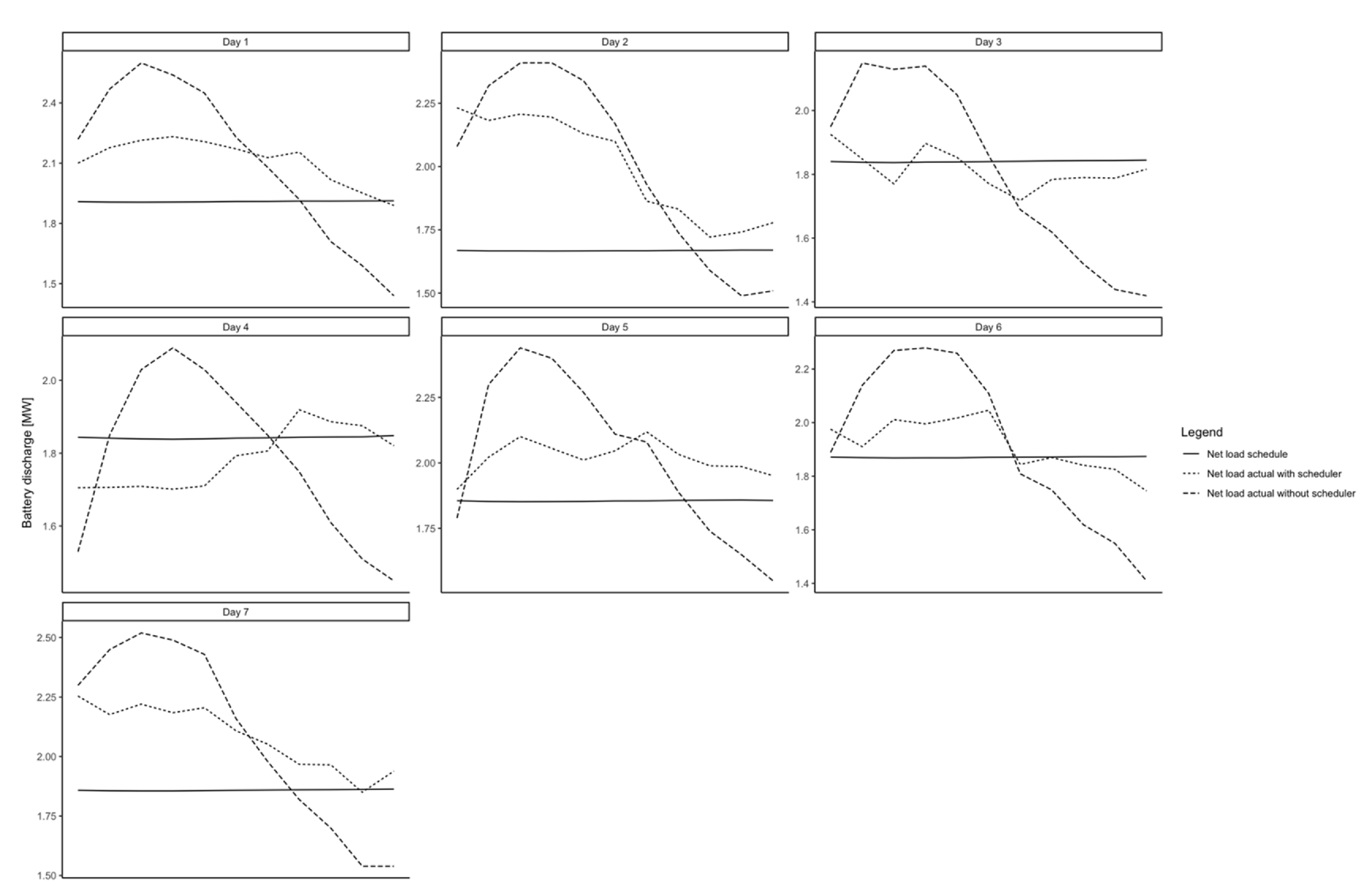
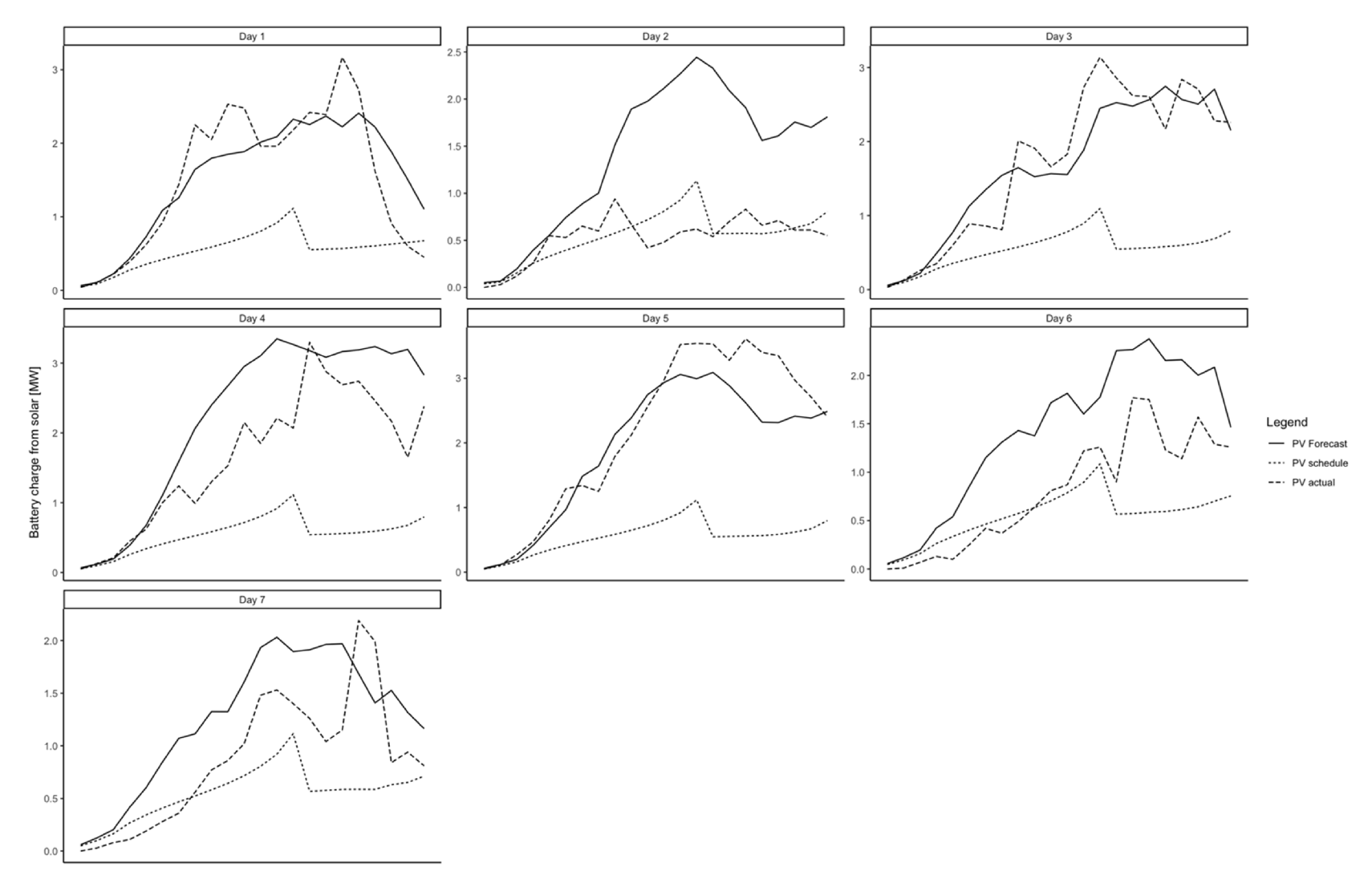
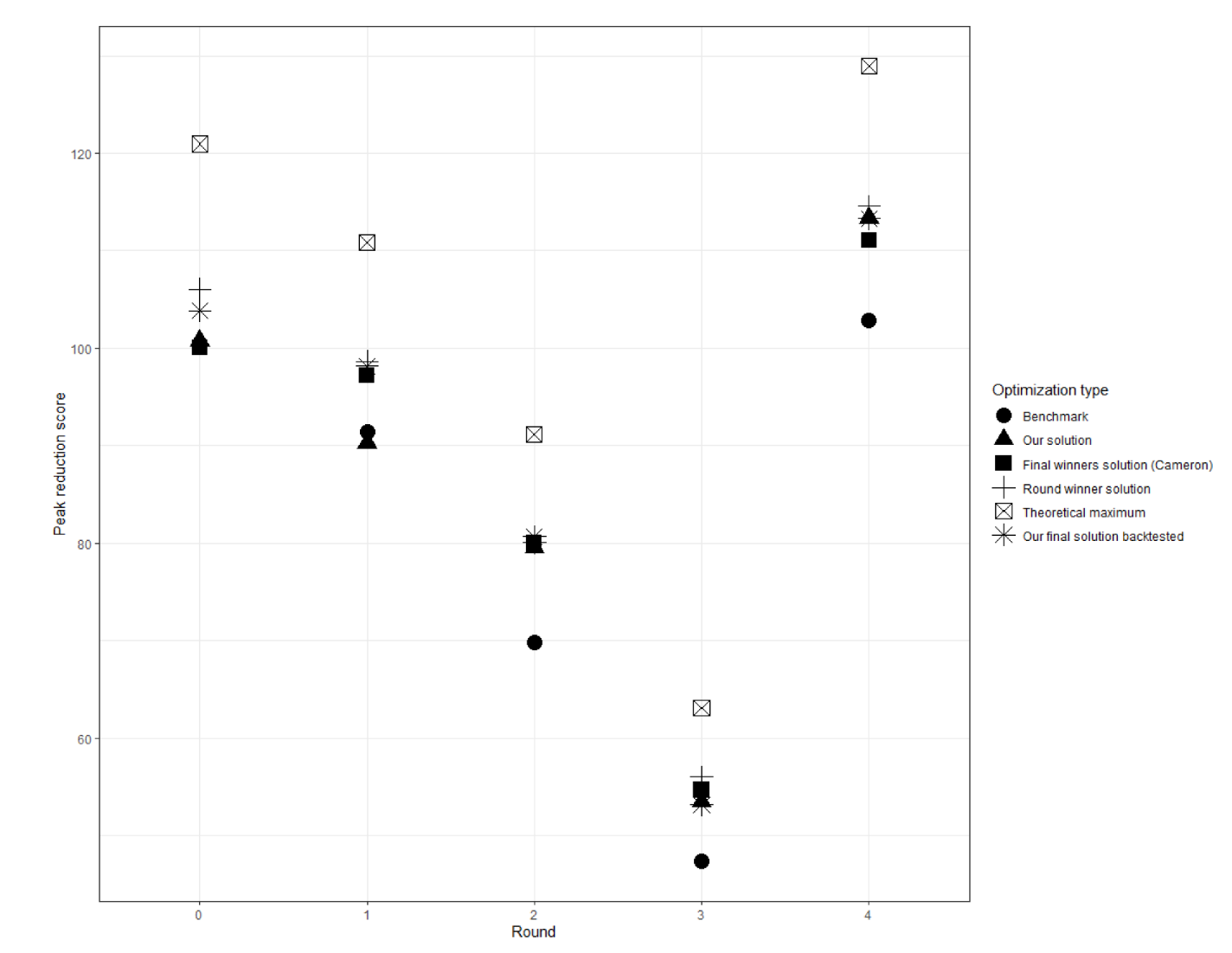
4.6.3. Battery Scheduler Results

In this section, we input our week-ahead demand and PV forecasts to both schedulers described in Section 3.4.1 and Section 3.4.2. The optimal schedule is then scored using the metric described in (27).

Table 8. Improvement in the weekly score from the scheduler with imperfect forecasts.

Round	Scheduler That Assumes No Error in Forecasts (a)	Scheduler That Accounts for Error in Forecasts (b)	Improvement in Score (b-a)	Best Possible Score
Round 0	99.65	103.83	4.18	120.97
Round 1	90.16	98.16	8	110.82
Round 2	76.17	80.69	4.52	91.15
Round 3	48.65	53.16	4.51	63.11
Round 4	99.57	113.33	13.76	128.98
Overall	82.84	89.83	6.99	103.0

shows various scores for all rounds for forecasts and actuals. The best possible score column represents the score obtained by feeding actual solar and load to the scheduler with perfect forecasts. Columns 2 and 3 are obtained by feeding forecasts to both schedulers. The difference in scores can be attributed to the improvements achieved by the scheduler that can consume forecasts with errors. We can clearly see that the weights and additional constraints applied to account for errors brought an improvement in scores across all rounds. We see that the highest improvement is achieved in Round 4, which can partly be attributed to the final scheduler parameters being optimized for the last round.

In Figure 3, we show the realized net load for schedules generated by both schedulers for round 4 for all 7 days. The planned net load (forecasts + discharge schedule) is relatively flat across peak hours. The realized net load, as shown, is not flat, but it is either above or below, which shows that there are errors in the forecasts. However, we can see that the realized net load is closer to the flat one when the errors are taken into account. For example, net load on day 3 with scheduler is very close to the net load flat line, which shows the improvement from that scheduler.

Figure 4 shows the actual PV output, charging schedule and PV forecasts for round 4 for all 7 days. Interesting observations can be made for days 2 and 3. Day 3 is a sunny day, and the forecast and actual are very close. As we scaled down the forecasts and limited the charging to the early morning, we slowly charged the battery and ramped it up during the afternoon. Day 2 turned out to be a non-sunny day, and the actual solar output was well below the forecasts. As the forecast has been scaled down and charging has been spread out across several hours of the day, we are able to charge most of it using solar output. A similar observation can also be made for day 7.

5. Discussion and Future Work

This paper describes an architecture for a battery scheduler that considers solar and demand forecasts. The solar and demand forecasts were generated by training machine learning models on historical data, whereas the scheduler was done with numerical optimization methods.

Figure 5 summarizes the achieved peak reduction scores compared to the leading competitors in the PoD challenge. The theoretical maximum reduction and the benchmark are also used to compare with other solutions. Our solution scores are submitted for each round in the challenge. However, we also improved our methodology as we progressed in the challenge, and the scores from the final round methodology are shown as back-tested solution scores. The actual score is dependent on the solar output and peak demand values for each round, as described in Section 4.6.1 and Section 4.6.2. As the methodology got refined, the final round’s back-tested scheduler would have achieved first place in the competition.

5.1. Improved Forecasting Framework

Our efforts to improve forecasting performance can be categorized into enriching the feature set and sophisticating the modeling.

5.1.1. Additional Input Features

Regarding solar modeling improvements, one of the most immediate steps to take is assuming the panel geometries and technologies based on several daily power production curves. This could then be utilized to model the tilted irradiance, that could potentially be a better predictor than the NWP GHI value at the grid points.

Throughout the competition, we used generation data of the Newton Downs solar farm as a proxy to the rooftop solar generation of the area. Although proven to add value to the demand modeling, this is only a rough estimation. Adding actual data of rooftop solar generation and considering the trends of capacity growth throughout the modeling period would yield a more accurate demand forecasting and thus better battery scheduling results.

5.1.2. Sophistication of Modeling

The following modeling techniques were utilized for the ML part of the work: Linear Regression, Lasso Regression, Random Forest, Extra Trees, XGBoost and Feed-Forward Neural Networks. These were tested under the same pipeline. Nonetheless, there is a possible improvement for the research to explore more sophisticated algorithms, such as deep learning, especially LSTM-type architectures.

In the demand forecasting approach, one could explore incorporating probabilistic load forecasts instead of simple point forecasts to add uncertainty information that could benefit the battery scheduling. Similarly, a separate peak hour forecasting module could ensure more reliable demand patterns to be used in battery scheduling. When it comes to forecast combinations, training a meta learner model, even a simple linear combination on top of the individual model forecasts, is something worth exploring. One must be cautious, even if the individual forecasts are properly calibrated, the combined forecast might not be [30].

5.2. Battery Scheduling Improvements

Using solar output predictions and demand forecasts, the scheduler optimizes for a maximum reduction in daily peak and charging the battery with as much solar energy as possible. This is achieved by formulating two optimization models: one that accepts perfect forecasts or does not account for errors in forecasts, and another that accounts for potential errors in forecasts. By comparing the schedules generated by both schedulers for a given forecast, we conclude that the scheduler that accounts for forecast errors greatly improves the scores and achieves the desired objectives.

We have proposed several heuristics to compensate for forecasting errors. To determine the charging schedule, we apply heuristics to scale down the forecasts to account for overprediction. We also impose some ad hoc constraints on the rate of change in charging rates for different time periods in the day. To determine the discharge schedule, we apply heuristics on prioritizing for peak hours. We also allow for some deviations in the scheduled flat net load.

The heuristic method of using weights to scaling forecasts for charging and discharging has shown to be very effective in comparison to not accounting for errors. As the next steps, it would be very interesting to see if the weights derived from historical error distributions in forecasts can further improve the score. Further, it will also be interesting to apply these heuristics to achieve other objectives, such as revenue maximization or reducing deviations in the day-ahead schedule.

References

1. Cole, W.; Frazier, A.W.; Augustine, C. Cost Projections for UtilityScale Battery Storage: 2021 Update; National Renewable Energy Laboratory: Golden, CO, USA, 2021. [Google Scholar]
2. Elshurafa, A.M. The value of storage in electricity generation: A qualitative and quantitative review. J. Energy Storage 2020, 32, 101872. [Google Scholar] [CrossRef]
3. U.S. Department of Energy. Electric Power Industry Needs for Grid-Scale Storage Applications. Available online: https://www.energy.gov/sites/prod/files/oeprod/DocumentsandMedia/Utility_12-30-10_FINAL_lowres.pdf (accessed on 20 August 2021).
4. Mangalova, E.; Agafonov, E. Wind power forecasting using the k-nearest neighbors algorithm. Int. J. Forecast. 2014, 30, 402–406. [Google Scholar] [CrossRef]
5. Barta, G.; Borbely, G.; Nagy, G.; Kazi, S.; Henk, T. GEFCOM 2014-Probabilistic Electricity Price Forecasting. Intell. Decis. Technol. 2015, 39, 67–76. [Google Scholar]
6. Aggarwal, S.; Saini, L. Solar energy prediction using linear and non-linear regularization models: A study on AMS (American Meteorological Society) 2013–14 Solar Energy Prediction Contest. Energy 2014, 78, 247–256. [Google Scholar] [CrossRef]
7. Bouktif, S.; Fiaz, A.; Ouni, A.; Serhani, M.A. Optimal Deep Learning LSTM Model for Electric Load Forecasting using Feature Selection and Genetic Algorithm: Comparison with Machine Learning Approaches. Energies 2018, 11, 1636. [Google Scholar] [CrossRef] [Green Version]
8. Alfares, H.; Nazeeruddin, M. Electric load forecasting: Literature survey and classification of methods. Int. J. Syst. Sci. 2002, 33, 23–34. [Google Scholar] [CrossRef]
9. Hong, T. Short Term Electric Load Forecasting. Ph.D. Thesis, North Carolina State University, Raleigh, NC, USA, 2010. [Google Scholar]
10. Xie, J.; Liu, B.; Lyu, X.; Hong, T.; Basterfield, D. Combining load forecasts from independent experts. In Proceedings of the 2015 North American Power Symposium (NAPS), Charlotte, NC, USA, 4–6 October 2015. [Google Scholar]
11. Hong, T.; Fan, S. Probabilistic electric load forecasting: A tutorial review. Int. J. Forecast. 2016, 32, 914–938. [Google Scholar] [CrossRef]
12. Martinez-Anido, C.B.; Botor, B.; Florita, A.; Draxl, C.; Lu, S.; Hamann, H.F.; Hodge, B.-M. The value of day-ahead solar power forecasting improvement. Sol. Energy 2016, 129, 192–203. [Google Scholar] [CrossRef] [Green Version]
13. Theocharides, S.; Makrides, G.; Georghiou, G.E.; Kyprianou, A. Machine learning algorithms for photovoltaic system power output prediction. In Energycon-2018; IEEE: Limassol, Cyprus, 2018. [Google Scholar]
14. Theocharides, S.; Makrides, G.; Venizelou, V.; Kaimakis, P.; Kyprianou, A.; Georghiou, G. Pv Production Forecasting Model Based on Artificial Neural Networks (ANN). In Proceedings of the 33rd European Photovoltaic Solar Energy Conference and Exhibition, Amsterdam, The Netherlands, 25–29 September 2017. [Google Scholar]
15. Zhang, J.; Hodge, B.-M.; Lu, S.; Hamann, H.F.; Lehman, B.; Simmons, J.; Campos, E.; Banunarayanan, V. Baseline and Target Values for PV Forecasts: Toward Improved Solar Power Forecasting. In Proceedings of the IEEE Power and Energy Society General Meeting, Denver, CO, USA, 26–30 July 2015. [Google Scholar]
16. Hummon, M.; Ibanez, E.; Brinkman, G.; Lew, D. Sub-Hour Solar Data for Power System Modeling From Static Spatial Variability Analysis. In Proceedings of the 2nd International Workshop on Integration of Solar Power in Power Systems, Lisbon, Portugal, 12–13 November 2012. [Google Scholar]
17. Marty, C.; Philipona, R. The clear-sky index to separate clear-sky from cloudy-sky situations in climate research. Geophys. Res. Lett. 2000, 27, 2649–2652. [Google Scholar] [CrossRef]
18. Guannan, H.; Quixin, C.; Chongqing, K.; Pierre, P.; Qing, X. Optimal Bidding Strategy of Battery Storage in Power Markets Considering Performance-Based Regulation and Battery Cycle Life. IEEE Trans. Smart Grid 2016, 7, 2359–2367. [Google Scholar]
19. Hejazi, A.; Rad, M. Optimal operation of independent storage systems in energy and reserve markets with high wind penetration. IEEE Trans. Smart Grid 2014, 5, 1088–1097. [Google Scholar] [CrossRef]
20. Zeyu, W.; Ahlmahz, N.; Daniel, K.S. Optimal Scheduling of Energy Storage under Forecast Uncertainties. IET Gener. Transm. Distrib. 2017, 11, 4220–4226. [Google Scholar]
21. Friedman, J.H. Greedy function approximation: A gradient boosting machine. Ann. Stat. 2001, 29, 1189–1232. [Google Scholar] [CrossRef]
22. Genre, V.; Kenny, G.; Meyler, A.; Timmermann, A. Combining expert forecasts: Can anything beat the simple average? Int. J. Forecast. 2013, 29, 108–121. [Google Scholar] [CrossRef]
23. Fan, S.; Chen, L.; Lee, W.-J. Short-Term Load Forecasting Using Comprehensive Combination Based on Multimeteorological Information. IEEE Trans. Ind. Appl. 2009, 45, 1460–1466. [Google Scholar] [CrossRef]
24. Hong, T.; Wang, P.; White, L. Weather station selection for electric load forecasting. Int. J. Forecast. 2015, 31, 286–295. [Google Scholar] [CrossRef]
25. U.S. Energy Information Administration. Available online: https://www.eia.gov/energyexplained/units-and-calculators/degree-days.php (accessed on 1 October 2021).
26. Hong, T.; Pinson, P.; Fan, S. Global Energy Forecasting Competition 2012. Int. J. Forecast. 2014, 30, 357–363. [Google Scholar] [CrossRef]
27. Aldosari, M.; Grigoriu, L.; Sohrabpoor, H.; Gorji, N.E. Modeling of depletion width variation over time in thin film photovoltaics. Mod. Phys. Lett. B 2016, 30, 1650044. [Google Scholar] [CrossRef]
28. Western Power Distribution. Open Data Hub Homepage. Available online: https://www.westernpower.co.uk/innovation/pod (accessed on 20 August 2021).
29. Haben, D.S.; Energy Systems Catapult. Value in Energy Data Special: Presumed Open Data Challenge. 2021. Available online: https://www.westernpower.co.uk/pod-data-science-challenge (accessed on 20 August 2021).
30. Ranjan, R.; Gneiting, T. Combining probability forecasts. J. R. Stat. Soc. Ser. B 2010, 72, 71–91. [Google Scholar] [CrossRef] [Green Version]
Figure 1. Architectural design of the proposed approach.
Energies 14 07794 g001
Figure 2. Demand forecasts for Extra Trees, XGBoost, LightGBM, the combined forecast and the actual demand on a weekday (left), weekend day (middle) and holiday (right).
Energies 14 07794 g002
Figure 3. Net load realized using schedules generated from both schedulers.
Energies 14 07794 g003
Figure 4. Solar forecasts, actuals and charge profile for all 7 days in Round 4.
Energies 14 07794 g004
Figure 5. Peak reduction scores of our solution, the benchmark, and the competitors’ solutions in the 4 + 1 rounds. Rounds 3 and 4 correspond to Christmas and COVID lockdown periods, respectively.
Energies 14 07794 g005