
Forecasting for Battery Storage: Choosing the Error Metric


Abstract
: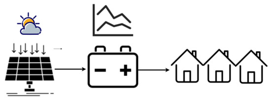
1. Introduction
- 1
- battery charging profile—For each half hour before 3:30 pm for each day of the upcoming week, prescribe how much charge the battery will take (up to a maximum of 2.5 MW over that half hour); and
- 2
- a battery discharging profile—For each half hour from 3:30 pm until 9 pm for each day of the upcoming week, prescribe how much the battery will discharge (up to a maximum of 2.5 MW over that half hour).
Competition Details
2. Data Provided
3. Materials and Methods
3.1. Approach
3.2. Forecasting Battery Charging Profiles
3.3. Forecasting Battery Discharge Profiles
3.3.1. Example Motivation
3.3.2. Deriving the Optimal Discharge Profile
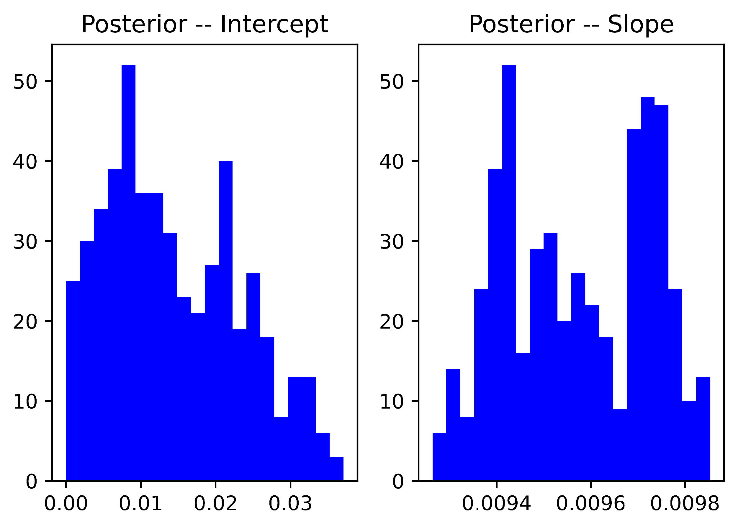
3.3.3. Error Metric
3.3.4. Forecasting
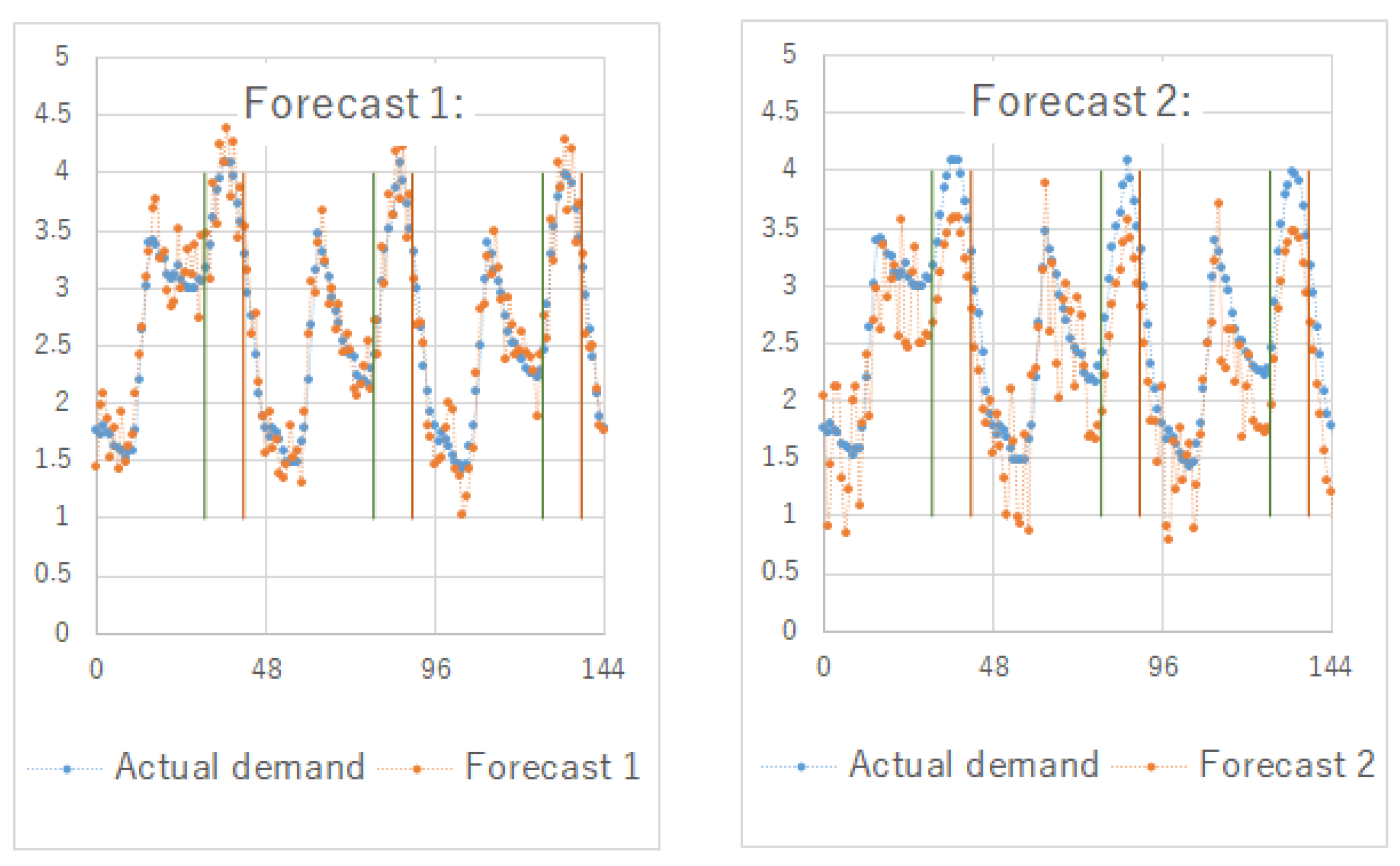
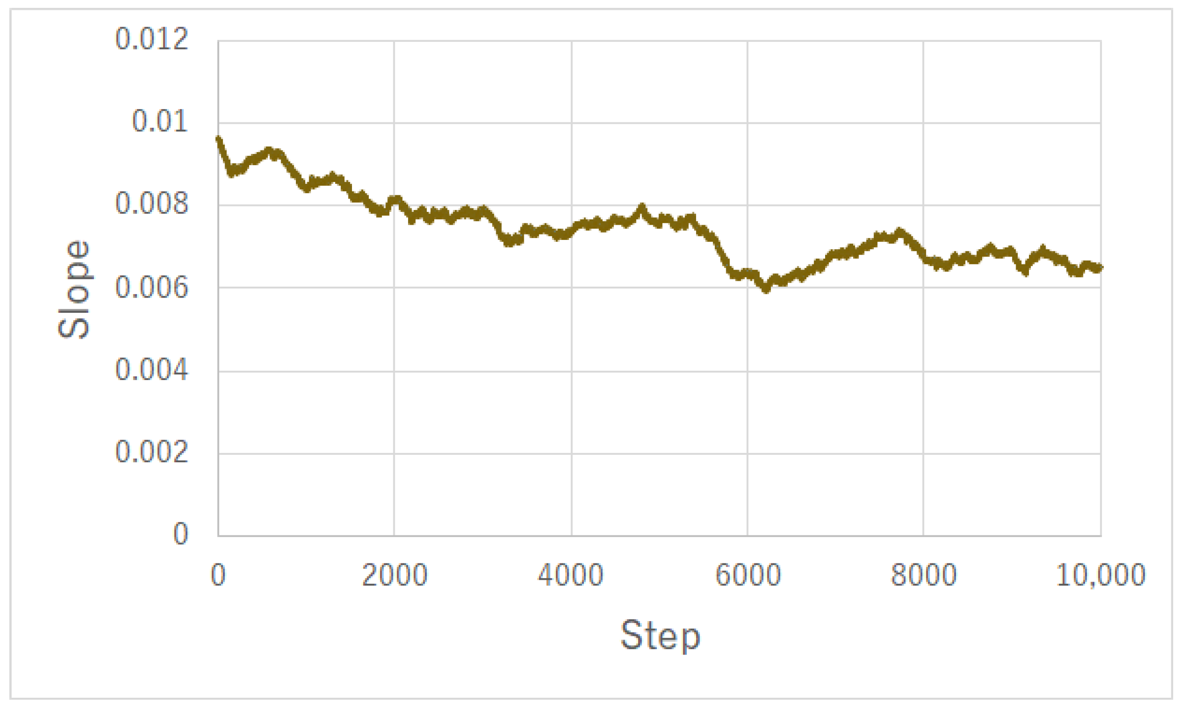
4. Results
4.1. Charging Profiles
4.2. Discharging Profiles
5. Discussion
6. Conclusions
Author Contributions
Funding
Institutional Review Board Statement
Informed Consent Statement
Data Availability Statement
Conflicts of Interest
References
- Box, G.E.P.; Tiao, G.C. Bayesian Inference in Statistical Analysis; Wiley: Hoboken, NJ, USA, 1973. [Google Scholar]
- Gilks, W.R.; Wild, P. Adaptive Rejection Sampling for Gibbs Sampling. J. R. Stat. Soc. Ser. C Appl. Stat. 1992, 41, 337–348. [Google Scholar] [CrossRef]
- Borghini, E.; Giannetti, C.; Flynn, J.; Todeschini, G. Data-Driven Energy Storage Scheduling to Minimise Peak Demand on Distribution Systems with PV Generation. Energies 2021, 14, 3453. [Google Scholar] [CrossRef]
- Haben, S.; Ward, J.; Vukadinovic Greetham, D.; Singleton, C.; Grindrod, P. A new error measure for forecasts of household-level, high resolution electrical energy consumption. Int. J. Forecast. 2014, 30, 246–256. [Google Scholar] [CrossRef] [Green Version]
- Hoffman, R.N.; Liu, Z.; Louis, J.F.; Grassotti, C. Distortion Representation of Forecast Errors. Mon. Weather Rev. 1995, 123, 2758–2770. [Google Scholar] [CrossRef] [Green Version]
- Kim, S.; Kim, H. A new metric of absolute percentage error for intermittent demand forecasts. Int. J. Forecast. 2016, 32, 669–679. [Google Scholar] [CrossRef]
- Tofallis, C. A better measure of relative prediction accuracy for model selection and model estimation. J. Oper. Res. Soc. 2015, 66, 1352–1362. [Google Scholar] [CrossRef] [Green Version]
- Makridakis, S. Accuracy measures: Theoretical and practical concerns. Int. J. Forecast. 1993, 9, 527–529. [Google Scholar] [CrossRef]
- Armstrong, J.; Collopy, F. Error measures for generalizing about forecasting methods: Empirical comparisons. Int. J. Forecast. 1992, 8, 69–80. [Google Scholar] [CrossRef] [Green Version]
- Rubner, Y.; Tomasi, C.; Guibas, L.J. A metric for distributions with applications to image databases. In Proceedings of the Sixth International Conference on Computer Vision, Bombay, India, 7 January 1998; pp. 59–96. [Google Scholar]
- Croston, J. Forecasting and Stock Control for Intermittent Demands. J. Oper. Res. Soc. 1972, 23, 289–303. [Google Scholar] [CrossRef]
- Nti, I.K.; Teimeh, M.; Nyarko-Boateng, O.; Adekoya, A.F. Electricity load forecasting: A systematic review. J. Electr. Syst. Inf. Technol. 2020, 7, 1–19. [Google Scholar] [CrossRef]
- Hyndman, R.J.; Koehler, A.B. Another look at measures of forecast accuracy. Int. J. Forecast. 2006, 22, 679–688. [Google Scholar] [CrossRef] [Green Version]
- Chai, T.; Draxler, R. Root mean square error (RMSE) or mean absolute error (MAE)? Geosci. Model Dev. 2014, 7, 1247–1250. [Google Scholar] [CrossRef] [Green Version]
- Microsoft. Define and Solve a Problem by Using Solver. Available online: https://support.microsoft.com/en-us/office/define-and-solve-a-problem-by-using-solver-5d1a388f-079d-43ac-a7eb-f63e45925040 (accessed on 18 August 2021).


| Error Metric | Forecast 1 | Forecast 2 | Optimal |
|---|---|---|---|
| RMSE—lower is better | 0.24 | 0.47 | 0 |
| MAPE—lower is better | 8.58 | 17.12 | 0 |
| ADPR—higher is better | 1.21 | 1.56 | 1.56 |
| W/c | Our Model | 49-pt Average | Regression | Benchmark |
|---|---|---|---|---|
| 16 October 2018 | 89.89% | 89.81% | 88.12% | 86.95% |
| 10 March 2019 | 77.36% | 76.05% | 78.01% | 71.03% |
| 18 December 2019 | 43.24% | 43.28% | 42.60% | 40.10% |
| 3 July 2020 | 96.73% | 96.69% | 96.08% | 94.32% |
| Average | 76.80% | 76.46% | 76.20% | 73.10% |
| Task Week | W/c | Our Model | RMSE-MP | RMSE-S | Benchmark |
|---|---|---|---|---|---|
| In-sample | last 35 days | 1.511 | 1.507 | 1.504 | 1.492 |
| 1 | 16 October 2018 | 1.478 | 1.376 | 1.359 | 1.436 |
| 2 | 10 March 2019 | 1.440 | 1.438 | 1.455 | 1.406 |
| 3 | 18 December 2019 | 1.366 | 1.360 | 1.331 | 1.305 |
| 4 | 3 July 2020 | 1.303 | 1.299 | 1.273 | 1.259 |
| Average | all 4 weeks | 1.397 | 1.368 | 1.354 | 1.351 |
Publisher’s Note: MDPI stays neutral with regard to jurisdictional claims in published maps and institutional affiliations. |
© 2021 by the authors. Licensee MDPI, Basel, Switzerland. This article is an open access article distributed under the terms and conditions of the Creative Commons Attribution (CC BY) license (https://creativecommons.org/licenses/by/4.0/).
Share and Cite
Singleton, C.; Grindrod, P. Forecasting for Battery Storage: Choosing the Error Metric. Energies 2021, 14, 6274. https://doi.org/10.3390/en14196274
Singleton C, Grindrod P. Forecasting for Battery Storage: Choosing the Error Metric. Energies. 2021; 14(19):6274. https://doi.org/10.3390/en14196274
Chicago/Turabian StyleSingleton, Colin, and Peter Grindrod. 2021. "Forecasting for Battery Storage: Choosing the Error Metric" Energies 14, no. 19: 6274. https://doi.org/10.3390/en14196274
APA StyleSingleton, C., & Grindrod, P. (2021). Forecasting for Battery Storage: Choosing the Error Metric. Energies, 14(19), 6274. https://doi.org/10.3390/en14196274