Reliability and Maintenance Management Analysis on OffShore Wind Turbines (OWTs)

Abstract

Due to the extreme marine operating environment, the remoteness from the maintenance base, and the expensive specialized accessibility and overhaul equipment needed (e.g., barges, boats, ships, and vessels), offshore O&M costs are greater than those for onshore-based installations. In the operation of wind farms, the main challenges are related to sudden and unexpected failures and downtimes. This paper has three main objectives. The first is to compare and optimize implementation techniques for maintenance strategies. The second is to analyze the cost-benefit of each maintenance strategy model. The third objective is to demonstrate the optimization and effectiveness of maintenance procedures and strategies recreated with stochastic and probabilistic life cycle cost (LCC) models, depending upon the degree of reliability and the maintenance process for offshore wind farms. The cost of operation and maintenance is directly dependent on failure rates, spare parts costs, and the time required by technicians to perform each task in the maintenance program. Calculations for each case study, with either light vessel/transfer boats (Alternative 1) or oilfield support vessels (Alternative 2), focused on the operational costs for transportation. In addition, each case study demonstrated which maintenance conditions and strategies are operational and optimal, and their corresponding cost–risk impacts. Results from this paper suggest that O&M costs are highly correlated with maintenance round frequency (offshore trips) and the operating costs for transportation by light vessel/transfer boat (CTV) and oil-field support vessel (FSV). The paper analyzes cumulative lifecycle costs and finds that for long-term life cycles (25 years), the implement of light vessels (Alternative 1) is more suitable and cost-effective. In contrast, oilfield support vessels (Alternative 2) are more expensive to operate, but they guarantee major capabilities, as well as the advantage of achieving the access levels need to efficiently operate. According to the results obtained by the outcome analysis, it can be concluded that the implementation of light vessels (Alternative 1) shows a lower overall LCC (<million $), which is mainly due to the fact that corrective maintenance and minor repairs are less costly. It should be noted that the cost of major repair operations with light vessels in Alternative 1 is still less than the high costs for minor repairs in Alternative 2 (with FSV).

1. Introduction

The continued growth in the size and complexity of offshore wind turbines means that more profitable O&M actions will be needed to optimize the upper ranges of robustness for RAMS, in order to fulfill the size increase [1].

Previous research has indicated that O&M constitutes up to 20–30% of the overall cost of OWTs during their lifetimes. However, lowering the O&M cost per unit power will rely on larger OWTs, due to the greater cost per failure of smaller OWTs, their high demand for palliative actions (e.g., corrective maintenance), and their loss of production during downtimes [1]. Therefore, increasing turbine size implies decreasing O&M costs. Larger OWTs provide a lower number of individual machines that need to be conserved and could therefore provide lower O&M costs [2]. The design and modeling of O&M costs is essential to the screening of cost-effective maintenance strategies and decision-making, as well as the development of specific methodologies for O&M. In addition, design and modeling increase trust for wind energy investors financing OWTs. Therefore, this analysis is a significant step for the growth of wind power [3]. The O&M costs quantified and measured in this paper are the cost for personnel, spare parts, and vessels required for the accomplishment of maintenance requirements of the wind farms. Normally, maintenance is understood as a general concept that includes all interventions (inspections, repairs, replacement of components/elements, etc.). The analysis of current and previous O&M strategies for OWTs takes into account industrial achievements made in the oil and gas industry and the manufacturing industry in order to identify the most important functional drivers for O&M planning, and management for OWTs. Thus, previous trials and achievements in other industries act as an input driver for O&M in the offshore wind industry.

To gain insight into current advances in O&M knowledgebase standardization, offshore wind farm models are based on today’s state-of-the-art OWTs, approximately 25 years after the first generation of conventional OWTs was designed, manufactured, and installed.

On the other hand, the use of larger wind turbines generates much greater uncertainty. Operation and maintenance costs represent a large part of the total life cycle cost (LCC), with operation and maintenance costs being approximately 22 to 40% of the overall total cost of an offshore wind farm [4,5]. Those costs are related to the risk cost incurred by the profit lost due to downtimes of OWTs.

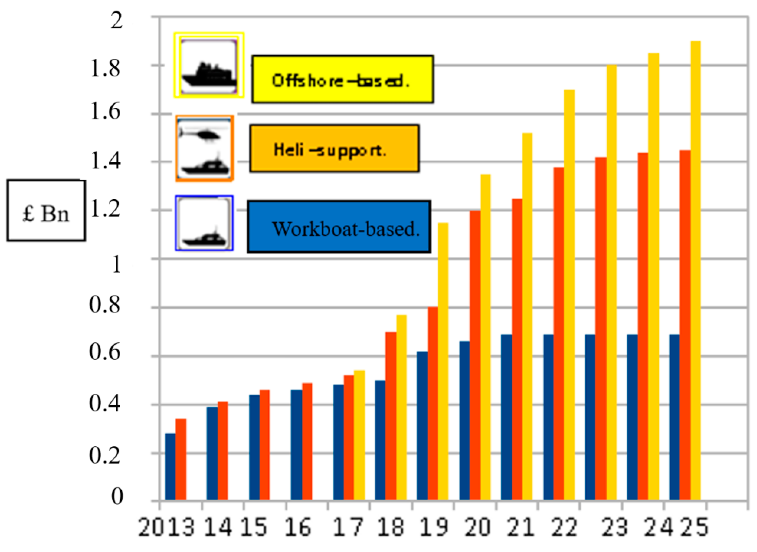
O&M activities account for around ¼ of the life-time costs of a regular offshore wind farm. Over the next twenty years, offshore wind O&M will turn into a significant industrial sector in its own right [3]. For instance, in the UK government’s forecasts for the deployment of offshore wind, O&M activities for more than 5500 OWT’s could be worth almost £2bn/year by 2025. The graphs are shown below in Figure 1.

Figure 2 represents a simple understanding of O&M research results for common offshore wind projects at different distances from the nearby O&M harbor. From the analysis, the junction points are at around 12 nautical miles (NM) (to have helicopter support) and at 40 NM (to trigger offshore wind-based strategies). However, it is vital to remember that there also many site-specific external aspects (environmental conditions, aviation regulations, safety considerations, and suitability) of existing ports that affect decisions about the exact positions of these junction points [3].

On the other hand, the prominence and challenges of O&M for OWTs are recognized in both academia and industry. The availability of OWTs is much less favorable and their costs can be more than 1.5 times higher than onshore wind. Furthermore, onshore wind turbines are capable of achieving 95–99% availability and producing electricity at a reasonable price in the market. There is clear cost reduction potential for O&M, which contributes around 30% of the total cost of offshore wind.

The emphasis of this document is to research and develop methods to improve and optimize the efficiency of operation and maintenance in offshore wind farms. Efficiency is related to the optimization of maintenance organization in offshore wind farms. The decrease of O&M costs is directly addressed in this document and the research results are supportive.

The research presented throughout this document analyzes the existing approaches and methods used for access, design, operation, maintenance planning, and life cycle engineering in offshore wind farms.

1.1. Challenges and Solutions for OWT Maintenance Activities

1.1.1. Weather Conditions

The meteorological window is represented in the model by a time series accounting for significant wave height and wind speed when determining the hourly time. The weather forecast notes when a given set of offshore or marine activities (operations, construction, etc.) can be carried out within their maximum limits for wave height, wind speeds, etc. Specifically, marine operations are planned based on a reference period; the operation reference period is (TR) = planned operation period (TPOP) + estimated maximum contingency time (TC) [6]. Incorporating wave height and wind speed into a weather window is crucial to ensuring the accessibility of offshore wind farms. For operations to be considered not limited by meteorological factors, it is necessary that the planned operating time (TPOP) be less than 72 h and the reference period (TR) be less than 96 h.

The meteorological time series are created using a Markov chain model based on historical meteorological record input data from the specific site of an offshore wind farm. The Markov chain model reproduces and recreates random time based on models and estimated stochastic probabilities [4].

Failure occurrence can fit an exponential probability distribution dependent on failure rates. Given the failure rates $\lambda$ (e.g., ${\lambda }^{\mathit{year}0—4}=1,$ ${\lambda }^{\mathit{year}5—10}=0.75,$etc.) for a component/element in an OWT, the distribution probability function for the time duration $\Delta t$ until a failure happens on that explicit component/element, is set as:

$$p\left(\Delta t\right)=\lambda e^{\lambda \mathsf{\Delta }t}$$

(1)

where (Δt) is the time interval until the next fault. Two cases are defined:

○

At the beginning of the simulation, the OWT components at the time that the “first failure” occurs are extracted independently of the exponential probability distribution, considering the relevant failure rate as an input parameter;

○

After a corrective maintenance process, when the next failure occurs in the maintained element, the distribution is extracted based on the failure rate relevant for this task and the current time. Therefore, feedback is provided for a corrective maintenance entry.

The maintenance model, therefore, is able to repeat simulations. Each one takes weather scenarios as diverse and random, and uses arbitrary times for failures to account for doubt in the times for failure rates and weather effects [7].

1.1.2. Weather Delays and Repair Timing

The total downtime per failure is the sum of the downtime originating because of:

○

Waiting for appropriate weather window conditions;

○

Queuing resulting from a lack of maintenance technicians;

○

Repairs in the OWTs.

Safety weather window and work shift constraints create expected maintenance delays, which are statistically determined for the given time duration (r_m & r_M) based on the environmental time series sum for the offshore location, with the vessels considered limited by wave height and wind speed [7].

Downtime repair comprising of waiting for weather (without the effect of queuing) is referred to as $d_m^s$ (minor repairs) and $d_M^s$(major repairs). The average failure rate (${\lambda }^S$) and repair time ($d_{CM}^s)$ per failure and per season is calculated as:

$${\lambda }^S={\lambda }_m^S+{\lambda }_M^S$$

(2)

$$d_{CM}^S=\frac{{\lambda }_m^S{d}_m^S+{\lambda }_M^S{d}_M^S}{{\lambda }^S}=\frac{1}{{\mu }^S}$$

(3)

where $\mu$^S is the resulting repair rate [8].

1.1.3. Accessibility

As stated above, both wave height and wind speed are essential to guaranteeing the safety and accessibility of an offshore wind farm. Accessibility itself is particularly essential for offshore wind power systems, to guarantee reduction of the great financial risks due to doubts to the accessibility and reliability of OWT [9].

Maintenance technicians’ transportation to the OWTs shall be carried out by workboats, which are limited by wave height [8].

1.1.4. Operation and Maintenance Plan

Maintenance planning is the prioritization of maintenance tasks ahead of available resources (for example, personnel, maintenance equipment, and spare parts). Maintenance planning involves all maintenance tasks, and the optimization process can achieve great savings. Mainly, cost savings are correlated with current assets (fuel, mobilization costs, production losses, and logistics costs) [9].

Managing operation and maintenance activities to reduce OPEX (operating expenses) costs is one of the most decisive challenges of offshore wind farms, due to the distribution of maintenance varying with time depending on the performance of OWTs and their sub-assemblies, as well as the weather window. Thus, to determine operation and maintenance activities, project managers need to have a clear understanding of sub-assembly history, background, performance, and weather [9,10]

Maintenance program activity triggers are usually failures of a component/element or a time interval based on operational service principles.

1.1.5. Objectives

The O&M programs and models rely on condition monitoring (CM)-based technologies such as dynamic load characteristics, oil analysis, strain measurements, physical condition of the materials, acoustic monitoring, performance monitoring, etc., which are helpful for monitoring wind turbines. The primary research goal is oriented around the condition monitoring of wind turbines and CM data is used to decide on maintenance planning and strategies/alternatives to be implemented, as well as to define deterioration models and develop mathematical models. The second objective is operational and maintenance (O&M) cost reduction coupled with less downtime. Due to offshore wind farm locations being much further from shore, new challenges will emerge which may interfere with reducing O&M costs.

The third objective shall be to overcome such challenges to minimize O&M expenditure.

1.1.6. Condition Assessment and Condition Indicators

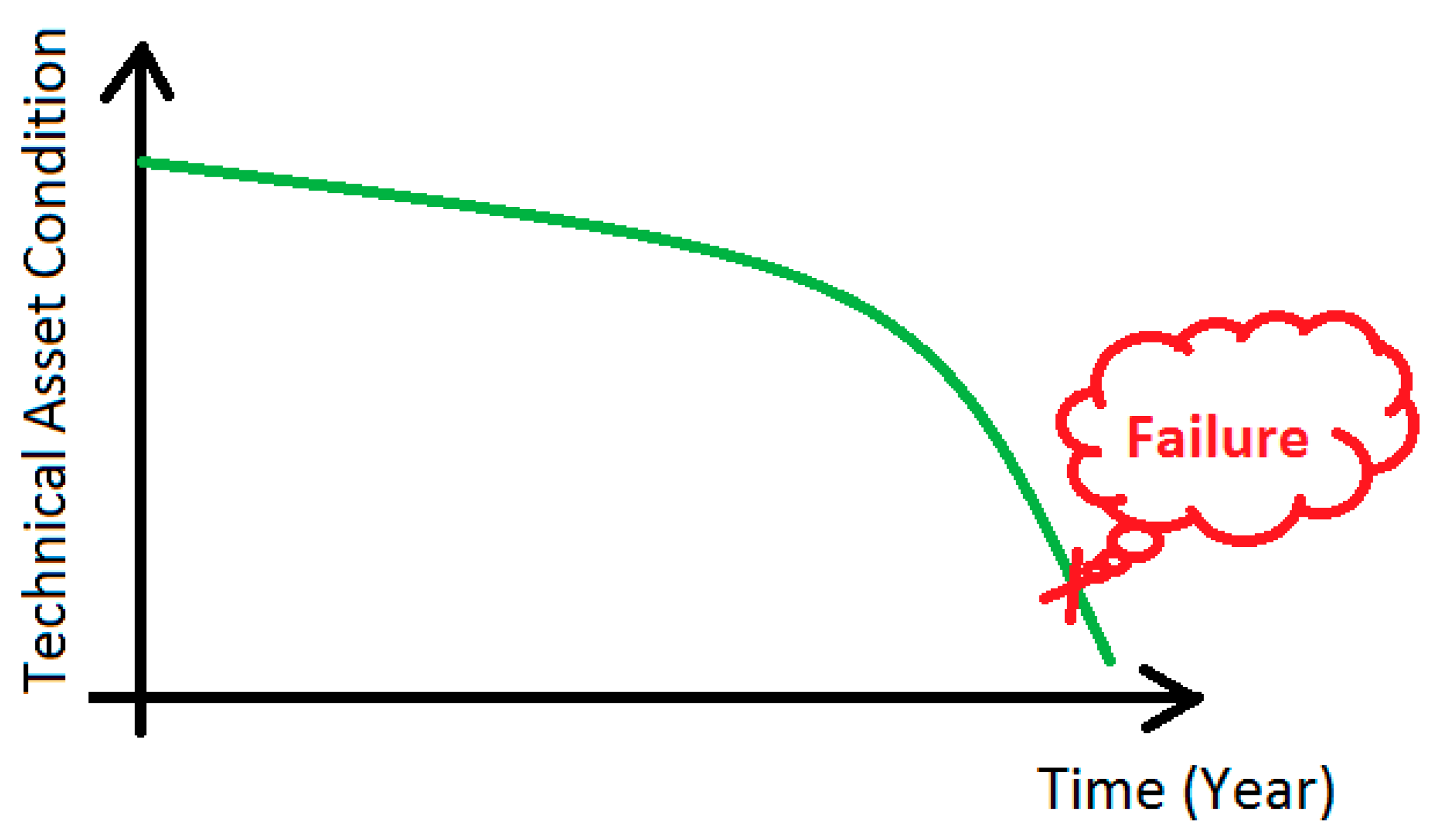
The degradation speed curve of the technical condition of a component/element is an on-going process from an “as new” condition until failure happens, as illustrated in Figure 3.

Very few, if any, condition monitoring methods give a direct and accurate description of the actual technical condition of the component/element. Methods used for the condition monitoring normally result in an indication of the technical condition of the components/elements. Energy companies have also carried out condition monitoring using visual inspections. As we know, visual inspections have higher uncertainty when giving precise knowledge of the point in time and momentum in space on an on-going deterioration curve. Besides O&M activities by power companies, visual inspection in modern industrial manufacturing plants has applied condition monitoring, based upon specific software solutions installed in each piece of equipment (for their respective production machines), which incorporate a tracking system for their technical condition.

Above all, O&M demands four key principles [11]:

• Maximize the level of turbine availability;
• Enable regular service and quick troubleshooting intervention;
• Enable component change, ensuring compatibility with the component exchanged;
• Ensure the cost effectiveness of the O&M concept.

Most publications have focused on quantifying the limitations of the three key O&M variables [10]:

• The distance of the service station;

  ○

  Service personnel stationed at an onshore site to service offshore platforms;

• Logistics to and from the offshore site;

  ○

  Service needs (e.g., vessels and helicopters);

• The availability of cranes or jack-ups;

  ○

  Adequate safe access to vessels for operational needs (e.g., replacing or transferring large components) [10].

1.2. Scope Work

This document reviews O&M management research on OWT operations and maintenance, including strategies, critical challenges and proposed solutions, on-site operations, and endpoints. Capable solutions are recognized with regard to the future development of O&M strategies. In addition, the negative effects of weather conditions, weather delays, repair times, and accessibility on offshore maintenance are presented. This analytical review presents a comprehensive overview of the OWT maintenance literature and provides a basis for improving O&M strategies and alternatives (1 vs. 2) in the future for offshore wind power installation facilities. To solve the information gaps, the comparison of scientific publications, technical reports and projects, and open databases has been used. The analysis is organized as follows. In Section 2, the research methodology, vessel data, personnel data, maintenance data, and online health monitoring are introduced and discussed, as well as the case studies (O&M Strategy 1 and O&M Strategy 2). Based on the designated maintenance methodology adopted, optimal maintenance direction-finding and scheduling are analyzed in Section 3. Several characteristics of the associated cost optimization problem are analyzed, including their advances, challenges, and targets. O&M strategies and alternatives, namely, O&M Alternative/Strategy 1 and O&M Alternative/Strategy 2 and their respective assumptions, are highlighted. A life cycle cost (LCC) analysis is conducted to evaluate both O&M alternatives/strategies (1 vs. 2) and determine which one is better. In Section 4, conclusions are drawn and discussed regarding operational and maintenance related issues from the outcomes obtained from the O&M alternatives-strategies analyzed, such as that a long-term life cycle (25 years) is more suitable for implementing Alternative 1, as it is more cost-effective. In contrast, it is more suitable to switch to Alternative 2 in order to guarantee major capabilities, as well as to have the advantage of achieving the access levels need to efficiently operate.

2. Methodology for Detailed Maintenance—Parameters Analyzed

2.1. Vessel Data

The O&M tasks to be carried out involve a fleet of diverse vessels. A standardized vessel consists of a vessel with a pre-established access system; therefore, maintenance technicians can easily access the OWTs. Some boats have additional capabilities (for example, cranes for lifting elements). There are questions about “high climate dependency” to access the OWT and “specific functional ship climate requirements” for the operational restrictions, in terms of the maximum possible, to access an OWT. Offshore vessels will not be able to participate in the maintenance tasks if the height of the waves or the speed of the wind exceeds their own meteorological limits, so they are not capable as such.

2.2. Personnel Data

The associated parameters associated with maintenance personnel are based on the availability of human resources. These resources focus on the number of maintenance technicians at different offshore site locations, as well as their own scheduled work shifts. Maintenance technicians are stationed at land or marine bases, while ships remain at sea for several days. Motherships have their own staff dedicated to the maintenance crew, who can operate the ships in their entirety for maintenance work purposes. The scheduled work preparation time for maintenance personnel is preset and identified by the scheduled work time (per shift combined + the n° of shifts/day).

2.3. Maintenance Data

On each component/element for the OWTs, the maintenance model relays one or more maintenance activities and rounds. To accomplish each maintenance activity, the model takes into account three kinds of assets:

• Vessel(s);
• Consumables and spare parts required;
• Maintenance work force.

Spare parts and consumables are included in the model by assigning them a delivery time and a cost linked to it. It is also necessary to detach all the maintenance tasks involving traveling to the offshore wind farm, which requires an offshore vessel to transport the maintenance technicians. However, some maintenance tasks require specific capabilities, such as high load capacity. For these maintenance tasks, vessels with additional capacity are required, which creates an additional cost for the LCC chain. All these factors have to be considered within the developed model [5].

2.4. Online Health Monitoring

OWTs demand appropriate online monitoring, in order to measure the industrial assets in real-time. Therefore, online data management for maintaining OWT is needed, to be exported to monitoring systems (i.e., SCADA, CMS, etc.). This online data measures reliability, availability, and maintenance from the control monitoring room of the OWTs’ OEM.

As we can see from the figure above, online asset management data gives robust health monitoring, allowing continuous monitoring of OWTs as well as ensuring that the OEM controls and operates in a cost-efficient and reliable manner, in order to guarantee the lowest LCC of the OWTs.

Description of the Case Studies.

We assume two different maintenance contracts, both lasting 20 years, including transport systems. Each contract carries out a hypothetical O&M strategy.

O&M Strategy 1:

The transport of maintenance crews offshore uses a light vessel (CTV) without access systems (MCA class 2), with 20 knots of cruising speed, a catamaran hull design, 12 personnel and 2 crews needed to operate, and suitable for 10–20 km offshore travels. This vessel has a limitation of 1.5 m in significant wave height, since availability cannot be over 98%.

O&M Strategy 2:

The transport of maintenance crews offshore uses an oilfield support vessel (FSV) with 12 knots of cruising speed and 18–68 personnel and crews needed to operate, suitable for long stays offshore up to 5–7 weeks. FSVs have dynamic positioning and access systems suitable for transferring heavier equipment to the OWT, so they can do heavier repair operations than Alternative 1. This vessel has a limitation of 4 m in significant wave height, so it is suitable for year-round maintenance. Hourly operation costs can be summarized as follows [10].

3. Analysis Review

3.1. Life Cycle Cost Analysis

Life cycle costs regarding O&M activities related to a general configuration can be calculated considering the following terms:

LCC = Capital Costs (C_cap) + Operating Costs (C_op) + Cost of Deferred Production (C_pr).

These terms have to be calculated yearly and corrected with a discount rate that accounts for inflation, interest rate, and investor risk, as is usual in economic analyses. A more general approach can be formulated as:

$$\mathrm{LCC}={\displaystyle \sum }_{\mathrm{i}}^{\mathrm{N}}\frac{{\left(C_{cap}+C_{op}+C_{pr}\right)}_{\mathrm{i}}}{{\left(1+r\right)}^{\mathrm{i}}}$$

(4)

where “N” is the life of the project in years (20).

This equation also complies with NORSOK O-CR-001 (for systems and equipment) and O-CR-002 (for production facilities). However, since this is an example comparing two different strategies for O&M in offshore wind power, not for equipment or production facilities, an optimum alternative solution will be used.

Now we compute the LCC for two alternatives, that is, for two different O&M strategies and two different transport concepts for maintenance crews:

Alternatives:

The two different maintenance contracts each last 25 years (the minimum life cycle of the OWT). Both alternatives are for an offshore wind location at a distance to the shore of 20 km (10,7238 NM) from where the wind farm is placed (i.e., WindFloat). Each O&M strategy will include different transport systems [11,12,13,14,15,16]:

○

O&M Strategy 1 (Alternative 1): Using a light vessel (CTV) without access systems. Parameters of Alternative 1 are summarized in

Table 1. Input data for Alternative 1 using a light vessel (CTV) without access systems.

Power of WT	8.4	MW
Number of OWT	3
Distance from shore	20	km
Water depth	85–100	m
N0 of Trips/round	30	Trips/Round
Cost per maintenance trip	2218.5	$/TRIP
Failure rate (minor repairs) %	75.00%
Failure rate (major repairs) %	25.00%
Cost of man-hours offshore	93.07	$/h
Number of crew members	4	people
Cost of electricity	50	$/Mwh
Offshore trips for minor repair	1	trips
Hours/WT preventive maintenance	36	h
Hours/WT corrective maintenance (minor repairs)	36	h

.

○

O&M Strategy 2 (Alternative 2) Using an oilfield support vessel (FSV). Parameters of Alternative 2 are summarized in

Table 2. O&M Strategy 2 (Alternative 2) using an oilfield support vessel (FSV).

Power of WT	8.4	MW
Number of OWT	3
Distance from shore	20	km
Water depth	85–100	m
N0 of trips/round	1	Trips/Round
Cost per maintenance trip (12 days)	216,500.1	$/trip
Cost per corrective maintenance trip (per days)	21,650.01	$
Failure rate (minor repairs) %	75.00%
Failure rate (major repairs) %	25.00%
Number of crew members (major repairs)	8	people
Number of crew members (minor repairs)	4	people
Cost of man-hours offshore	501.07	$/h
Number of crew members (preventive)	28	people
Cost of electricity	50	$/Mwh
Offshore days for minor repair	3	days
Hours/WT preventive maintenance	32	h
Hours/WT corrective maintenance (minor repairs)	36	h
Offshore days for major repair	3	days
Hours/WT corrective maintenance (major repairs) (2 shifts 12 h x 2)	72	h

.

3.2. Assumptions

The upcoming analysis requires a list of assumptions. The two different strategies will be compared based on the following assumptions. The preventive maintenance program shall be done every 3500 h (2 times/year), taking 2–3 days/WT per year. In this case study, we have N = 20 years of duration of the transport contract and, since this transport alternative is externally hired, capital costs are 0, so:

$$\mathrm{LCC}={\displaystyle \sum }_{\mathrm{i}=1}^{20}\frac{{\left(C_{op}+C_{pr}\right)}_{\mathrm{i}}}{{\left(1+r\right)}^{\mathrm{i}}}$$

(5)

Operating costs will be divided between preventive and corrective, since both are mandatory and the LCC of each needs different treatment:

$$\mathrm{LCC}={\displaystyle \sum }_{\mathrm{i}=1}^{20}\frac{{\left(C_{op}^{prev}+C_{op}^{corr}{C}_{pr}\right)}_{\mathrm{i}}}{{\left(1+r\right)}^{\mathrm{i}}}$$

(6)

Relevant operating costs for comparing both alternatives are due to transportation strategies (including energy/fuel consumption) and man-labor hours. Spare parts, insurance, and other operating costs are considered constant for both alternatives.

We will consider a failure rate that changes with time to be more realistic, since WTs are more likely to fail the older that they get, following the bathtub curve approach:

$$\begin{array}{l}{\lambda }^{year0—4}=1;{\lambda }^{year5—10}=0.75;{\lambda }^{year11—16}=0.5;{\lambda }^{year17—20}=0.75\\ {\lambda }^{year21—25}=1\mathrm{in}\mathrm{failures}/\mathrm{year}.\end{array}$$

This equation comprises minor and major failures (needing minor and major repair). In this context, we define failure as an event that prevents the WT from producing energy at all.

Preventive maintenance will be based on planned maintenance rounds, which are also assumed to change with time, and according to the feedback from each settled and applied maintenance program, in order to better optimize O&M strategies with the failure rates:

○

From year 1–8: 2 Maintenance rounds/year.

○

From year 9–20: 4 Maintenance rounds/year.

The cost of man-labor in offshore conditions is considered to be 250 $/h.

During corrective maintenance, minor failures on each WT will take 1 day to repair (9 h of offshore labor by 1–4-man crews); major failures will take 3 days offshore with accommodation, in 4 shifts (4 × 4-man crews, 8 h each) [12].

3.3. Operational Cost Results

The hourly costs (costs of operation) of each alternative are shown in the

Table 3. Hourly cost for Alternative 1.

Transport Alternative 1: CTV MCA CLASS C
HIRE AND FUEL
	Fuel costs $/ton	381	$/ton
	12 h trip rental	1905	$
	Fuel costs 2 × 20 km trip (2 × 10.71 NM; 0.12 tons of fuel used)	45.72	$
	Fuel costs on location 8 h, no heavy seas and light sailing (0.4 MT fuel used)	152.4	$
	TOTAL CTV INCLUDING FUEL	2103.12	$/trip
WORKING HOURS PER WT	3 × 4-man teams working 9 h	36	h/WT

Alternative 1 cost of transportation per hour of O&M work is equal to 58.42 $/h.

and

Table 4. Hourly cost for Alternative 2.

Alternative Transport Alternative 2: FSV
HIRE AND FUEL		DAYS	12
	Fuel costs $/ton		381	$/ton
	12 day trip rental		152,400	$
	Fuel costs 2 × 20 km trip (2 × 10.71 NM at 12 knots, 29 tons/24 h fuel used)		952.5	$
	Fuel consumption at port (1 day for picking and leaving shifts)		571.5	$
	Fuel costs on location, no heavy seas and light sailing (6.5 MT/24 h fuel used) during 12 days		29,718	$
	TOTAL FSV INCLUDING FUEL		183,642	$/trip
WORKING HOURS PER WT	4 × 7-man maintenance team working 8 h in 3 shifts (4× morning, 4× afternoon, and 3× night) working 12 days		32	h/WT

Alternative 2 cost of transportation per hour of O&M work is equal to 5738.8 $/h.

below:

Both case studies (Alternatives 1 and 2), are calculated using the same distance to the shore, at 20 km, from where the wind farm (i.e., WindFloat) is placed.

3.4. Cost of Deferred Production

According to NORSOK O-CR-001 and O-CR-002, the costs of deferred production can be calculated, in general form, as:

$$C_{pr}=\lambda \ast p\ast D\ast L$$

(7)

where $\lambda$ is the failure rate per year (which is assumed to be varying with time, as stated above), p is the probability of interrupted production reduction, D is the duration of production reduction (downtime), and L is the production loss per time unit.

• $\lambda$ is assumed to be: ${\lambda }^{year 0—4}=1$; ${\lambda }^{year 5—8}=0.75$; ${\lambda }^{year 9—12}=0.5$; ${\lambda }^{year 13—16}=0.75$; ${\lambda }^{year 17—20}=1$.
• $P$ is taken as 0.01, so a 1 × 100% train configuration is assumed.
• L is taken as 8.4 MWh, which is the power of a WT wind farm (for example, WindFloat) every hour, so all production is assumed to stop at every failure. The price of electricity is taken as 50 $/MWh [13].

The downtime (D) is the main difference between the two alternatives. Alternative 2 can have a much higher availability and lower downtime. For this, we follow some of the concepts and procedures indicated by [11].

In general, the failure rate during a season (year) can be divided into failure needing major repair (change of rotor blades) and minor repair (change of lubricating boxes):

$${\lambda }^s={\lambda }_m^s+{\lambda }_M^S=\frac{1}{MTBF}$$

(8)

We will assume $\lambda ={\lambda }_m+{\lambda }_M$ = 0.75$\lambda$ + 0.25$\lambda$ failures/year, so 75% of failures are solved with minor repair operations, while 25% need major repair. When considering both major and minor repairs, the repair time per failure MTTR can be calculated as (this downtime includes waiting for the weather window, but does not include queuing, when maintenance crews are not available to repair the failures, or logistics, such as waiting time for spares; these are supposed to be constant in both alternatives):

$$d_{CM}^s=\frac{{\lambda }_m^S\ast d_m^s+{\lambda }_M^s\ast d_M^s}{{\lambda }^S}=\frac{1}{{\mu }^S}=MTTR$$

(9)

Where $d_m^s$ is the mean downtime due to failure needing minor repairs, $d_M^s$ is the mean downtime due to failures needing major repairs, and ${\mu }^S$ is the average repair rate.

For Alternative 1, we will assume that $d_m^s$ is around 3 days/turbine and $d_M^s$ is large, in the order of 20 days/turbine, since no major repairs can be done with these vessels. Notice that in this case, we would need another vessel for that purpose (major repairs), which is outside of the scopes of the contract. So, considering the time varying failure rate per year:

$$d_{CM}^{alt1}=\frac{0.75\ast 3+0.25\ast 20}{1}=7.25\frac{days}{failure}=\frac{1}{{\mu }^{alt1}}$$

(10)

For Alternative 2, we will assume that $d_m^s$ is around 1.5 days/turbine, since 24 h shifts can be considered, and $d_M^s$ is in the order of 10 days/turbine, since major repairs can be done with the FSV vessel.

$$d_{CM}^{alt2}=\frac{0.75\ast 1.5+0.25\ast 10}{1}=3.625\frac{days}{failure}=\frac{1}{{\mu }^{alt2}}$$

(11)

With these assumptions, we can finally obtain an estimate for the costs of deferred production. A more detailed calculation on downtimes, including queuing issues, is discussed in [10], by means of Markov chain models.

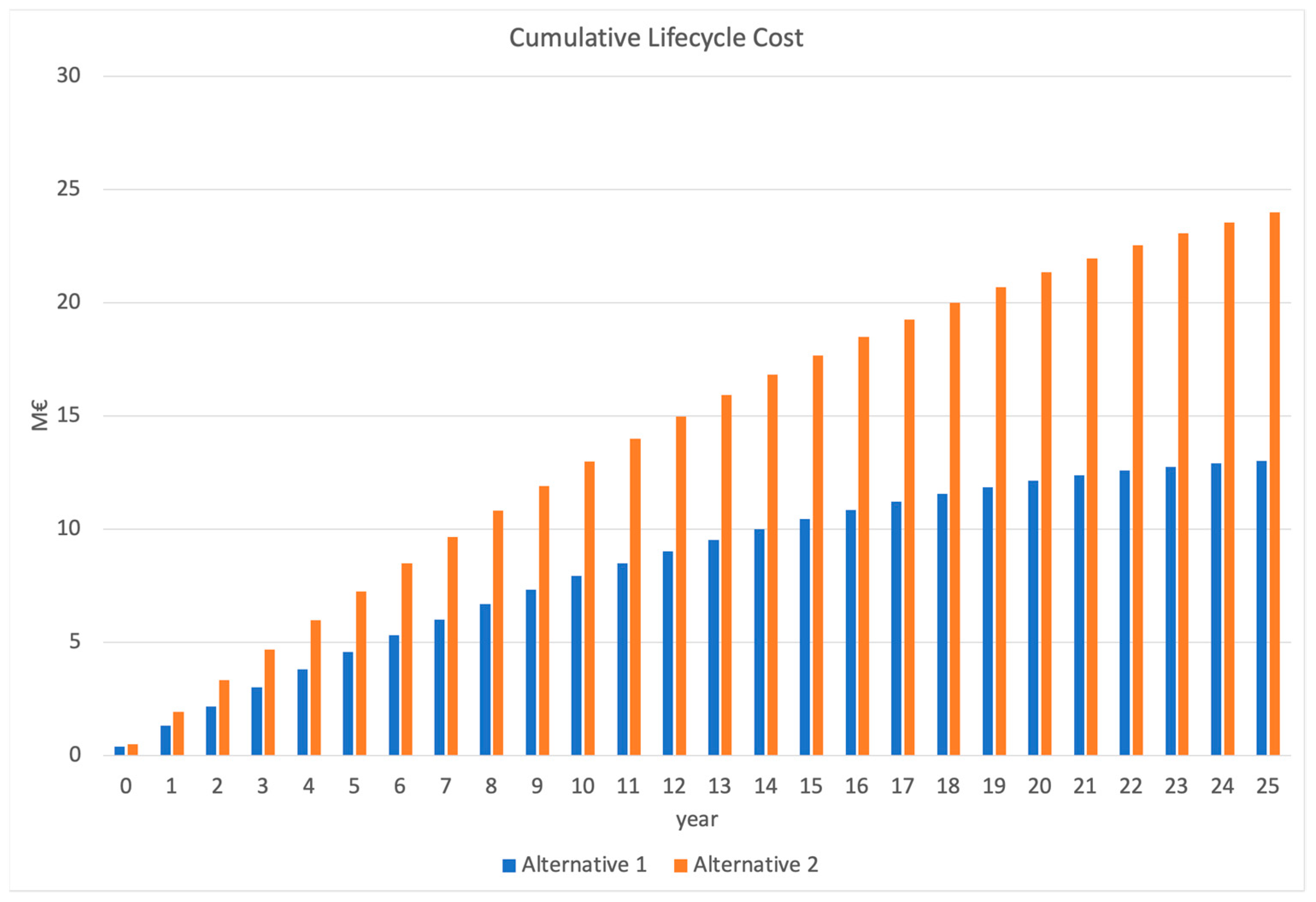
The expressive summary for the whole life cycle of the project, comparing the given O&M options, is showed in

Table 5. Comparison between Alternatives 1 and 2.

	Corrective
	Minor Repairs			Major Repairs
	Transport	Man-labor	Total	Transport	Man-labor	Total
1	$51.14477	$77.24208	$128.38685	$1.99645656	$998.05372	$2.99451028
2	$499.11414	$415.85572	$914.96986	$1.66371380	$831.71143	$2.49542523
Overall Life Cycle Costs (Discounted)
1	$13.44641325
2	$24.03934295
	Preventive
	Transport		Man-labor			Total
1	$174.25252		$1.32804120			$1.1537868
2	$833.90240		$4.58711952			$3.75321712
Deferred Production Costs
1	$93.59827
2	$46.79913

and Figure 4:

Alternative 1 shows lower overall LCC (less than a million USD); this is mainly because corrective maintenance due to minor repairs is less costly due to the characteristics of the chosen transportation (CTV). The penalization in the costs of major repair operations (120%) is not enough to compensate for the high costs for minor repair of Alternative 2 (FSV).

Deferred production costs are not high enough to be decisive in the selection between alternatives. If this were an oil and gas project, this may have been different.

This way of obtaining LCC leads us to average values. In order to assess the variability of these assumptions and costs, a Monte Carlo simulation can be carried out on the decisive parameters (cost of man-labor, cost of fuel, costs due to major repairs, downtimes, failure rates), assuming a variance of those, with a certain distribution (usually a triangular one, with the mode at the center). After this simulation, we can obtain an estimate of the uncertainty and sensitivity of some assumptions, such as quantities for the obtained LCC or the probability that these are in a certain range, confidence intervals, or any other quantification of uncertainty. This though, is beyond the scope of this article.

4. Conclusions

The potential impact from maintenance at the operating and logistical level (flexibility, throughput time, quality management, etc.) is considerable, and, therefore, the financial impact of maintenance can be substantial.

This work analyzes decreasing the O&M cost depending upon failure rates, downtimes, the timing needed for each maintenance schedule work activity, and the associated spare part costs.

The O&M cost results proved a great variability in cost of transportation between each alternative. In Alternative 1, the cost of transportation per hour of O&M work is 58.42 $/h, but for Alternative 2, it goes up to 5738.8 $/h. In summary, the total O&M cost of transportation per hour of O&M work differs from Alternative 1 to 2 by 5680.38 $/h, showing that a reachable decrease in O&M cost is highly dependent upon the technical assumptions set into the initial alternative/strategy and on the development of O&M requirement values (parameters and variables), which are key to recreating and covering the full spectrum of each case study.

Availability rises with a higher degree of accessibility and faster transportation times from support organizations. In contrast, the availability itself depends upon the O&M principles (effective working hours scheduled and number of technicians) set in each O&M strategy (Alternative 1 vs. Alternative 2).

In addition, as the cumulative lifecycle cost proves, for almost half of the life cycle (25 years), the costs-discounted are higher for Alternative 2 (using FSV) than for Alternative 1. Therefore, the long-term life cycle (25 years) is more suitable for implementing Alternative 1, as it is more cost-effective. In contrast, it is more suitable to switch to Alternative 2 in order to guarantee major capabilities, as well as the advantage of achieving the access levels needed to efficiently operate.

Increasing the size of OWTs demands a higher robustness of the O&M implementation, in comparison with traditional and conventional offshore wind farms.

Finally, the optimal O&M strategy maximizes availability at the lowest cost by ensuring safety and the best access to offshore wind farms, minimizing unscheduled maintenance activities, and carrying out scheduled maintenance tasks as efficiently as possible, ultimately resulting in the lowest possible LCOE.