A Modification of Newton–Raphson Power Flow for Using in LV Distribution System

Abstract

The Newton–Raphson (NR) method is still frequently applied for computing load flow (LF) due to its precision and quadratic convergence properties. To compute LF in a low voltage distribution system (LVDS) with unbalanced topologies, each branch model in the LVDS can be simplified by defining the neutral and ground voltages as zero and then using Kron’s reduction to transform into a 3 × 3 branch matrix, but this decreases accuracy. Therefore, this paper proposes a modified branch model that is also reduced into a 3 × 3 matrix but is derived from the impedances of the phase-A, -B, -C, neutral, and ground conductors together with the grounding resistances, thereby increasing the accuracy. Moreover, this paper proposes improved LF equations for unbalanced LVDS with both PQ and PV nodes. The improved LF equations are based on the polar-form power injection approach. The simulation results show the effectiveness of the modified branch model and the improved LF equations.

1. Introduction

A low voltage distribution system (LVDS) is responsible for providing electricity to end-users and connecting with its distribution transformer, which receives electricity from a medium voltage feeder. Many LVDSs are usually built-in radial structures because of reducing investment costs and simplifying coordination plans for protection devices [1]. Most LVDSs have unbalanced loads and have grounding resistances that range from 1 to several ohms [2]. To analyze LVDSs more accurately, load flow (LF) calculations should include neutral and ground conductors as well as grounding resistances.

Studies present various LF algorithms, such as the Gauss–Seidel (GS), forward–backward sweep (FBS), and Newton–Raphson (NR) methods to handle the LF with various applications and LVDS structures [1,3,4,5,6,7,8,9,10,11,12]. First, the GS method allows performing LF with complex variables by reducing the number of required calculations and avoiding the calculation of derivative equations. In [1], the GS method is applied to solve balanced LVDSs, whereas [3] presents the modified GS method for solving LFs in unbalanced LVDSs. Both [1,3] prove that the GS method has a very low computation time compared to the other methods.

Second, the FBS method is preferred by many authors [4,5,6] due to its simple programming for small-matrix calculation and its ability to guarantee convergence in radial LVDSs. In [4], an improved FBS method is presented for LF calculations in balanced LVDSs with weakly-meshed topology. In [5,6], the FBS method is used for LF calculations in unbalanced LVDSs.

Finally, the NR method is still frequently used for LF calculations in LVDSs. This method uses derivatives for approximation at each iteration. This method has precision and quadratic convergence properties, and the calculation requires less iterations [7,8,9,10,11,12]. The power injection-based approach used in [7,8,9] corresponds to the traditional Newton–Raphson method, whereas the current injection-based approach used in [10,11] was invented later by [12]. The latter approach tends to perform better because of the linearity of its current injection equations. Overall, [7,8,9,10,11] solve LFs in unbalanced LVDSs, but [12] is used for balanced LVDSs.

The advantage of each method was stated earlier. However, each method has its weakness as follows. The GS method may face uncountable processing time when loads or the number of nodes increase [1,3]. The FBS method used in [5,6] cannot be applied to meshed LVDSs. Although the improved BFS method in [4] can perform in balanced LVDSs with weakly meshed topology, it cannot perform in unbalanced LVDSs and can face non-convergence problems in meshed balanced LVDSs with heavy loads. The total processing time of the NR method will increase if it requires the inversion of high-dimensional matrices. Moreover, the NR method can perform poorly for ill-conditioned LVDSs [7,8,9,10,11,12].

There are some weaknesses of the aforementioned reviews [1,4,5,6,7,8,9,10,11,12]. Determining the balanced LVDSs in [1,4,12] is inaccurate because the loading of any LVDS is inherently unbalanced due to the many unequal single-phase loads and non-symmetrical spacings between conductors. Not determining the conductors, which include phase-A, -B, -C, neutral, and ground, together with the grounding resistances, can cause inaccuracies in the branch model [7,8,9,10,11]. In addition, Refs. 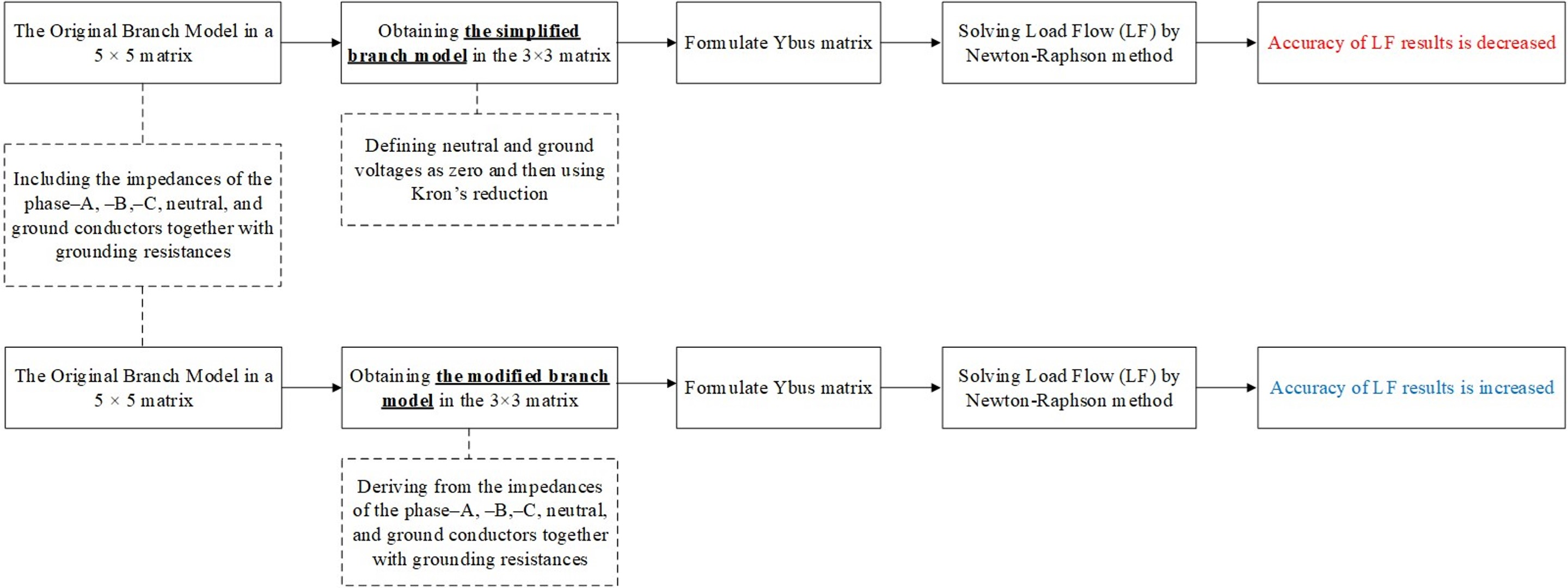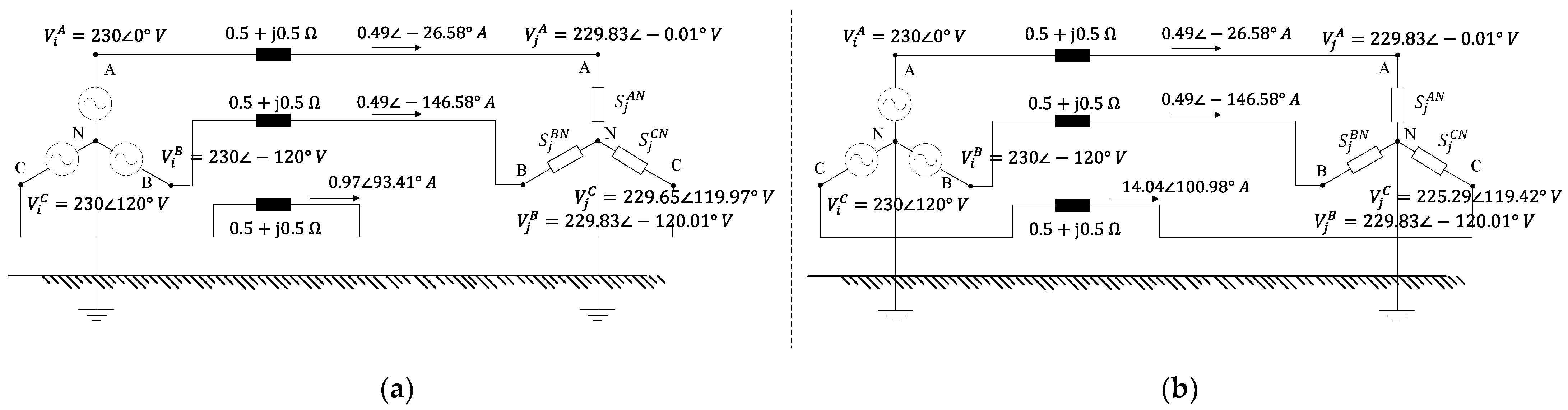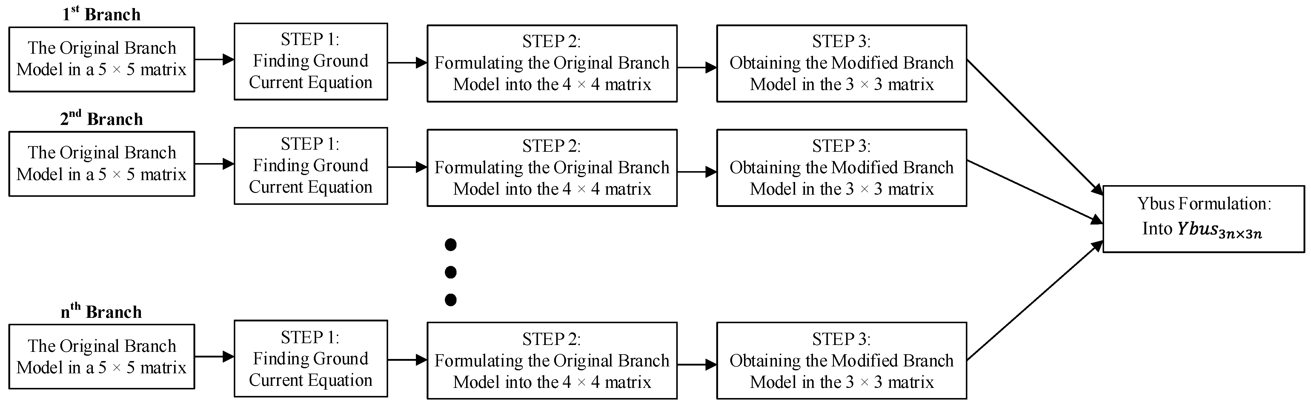[5,7] simplify the original branch model, which includes a 5 × 5 matrix of the phase-A, -B, -C, neutral, and ground conductors as well as the grounding resistances into a 3 × 3 matrix by defining the voltages of the neutral and ground conductors as zero and, after that, using Kron’s reduction. This leads to inaccuracies in the results from [5,7]. In [6,7,8,11], the LF calculations do not deal with LVDSs with PV nodes. Finally, [9,11] regulate the PV nodes using a simplification by which the voltage magnitude and real power output of each phase of PV node are regulated separately. However, the PV node must regulate the voltage magnitude and phase angle of each phase to be balanced, such as the connection of an advanced three-phase solar inverter [13] or a load-managing converter [14]. Finally, the current injection NR method with the modified 4 × 4 branch matrix can suffer from the lack of convergence in the LVDSs with PV nodes [10] where the 4 × 4 branch matrix neglects only the voltage existence of the ground conductor.

From the variety of all the methods previously reviewed, this paper chooses the NR method due to its quadratic convergence property and range of applications (for both radial or meshed LVDSs) [7,8,9,10,11,12]. Polar-form LF equations based on the power injection approach are applied because of the intuitiveness and convenience of their direct specification of node power injections [8]. The two modifications of this paper are proposed for the correction of the weaknesses of the aforementioned reviews [1,4,5,6,7,8,9,10,11,12], as expressed in the following:

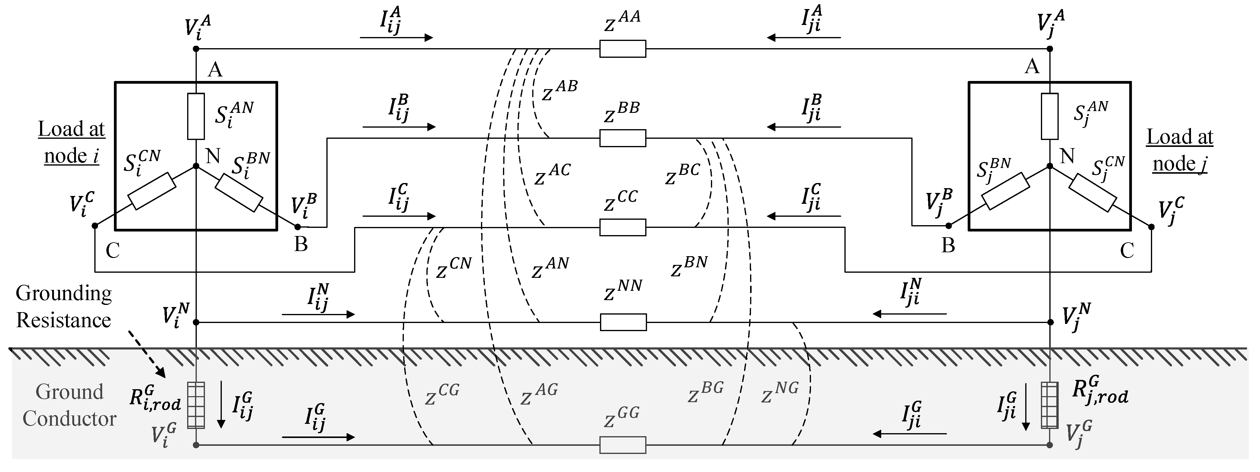
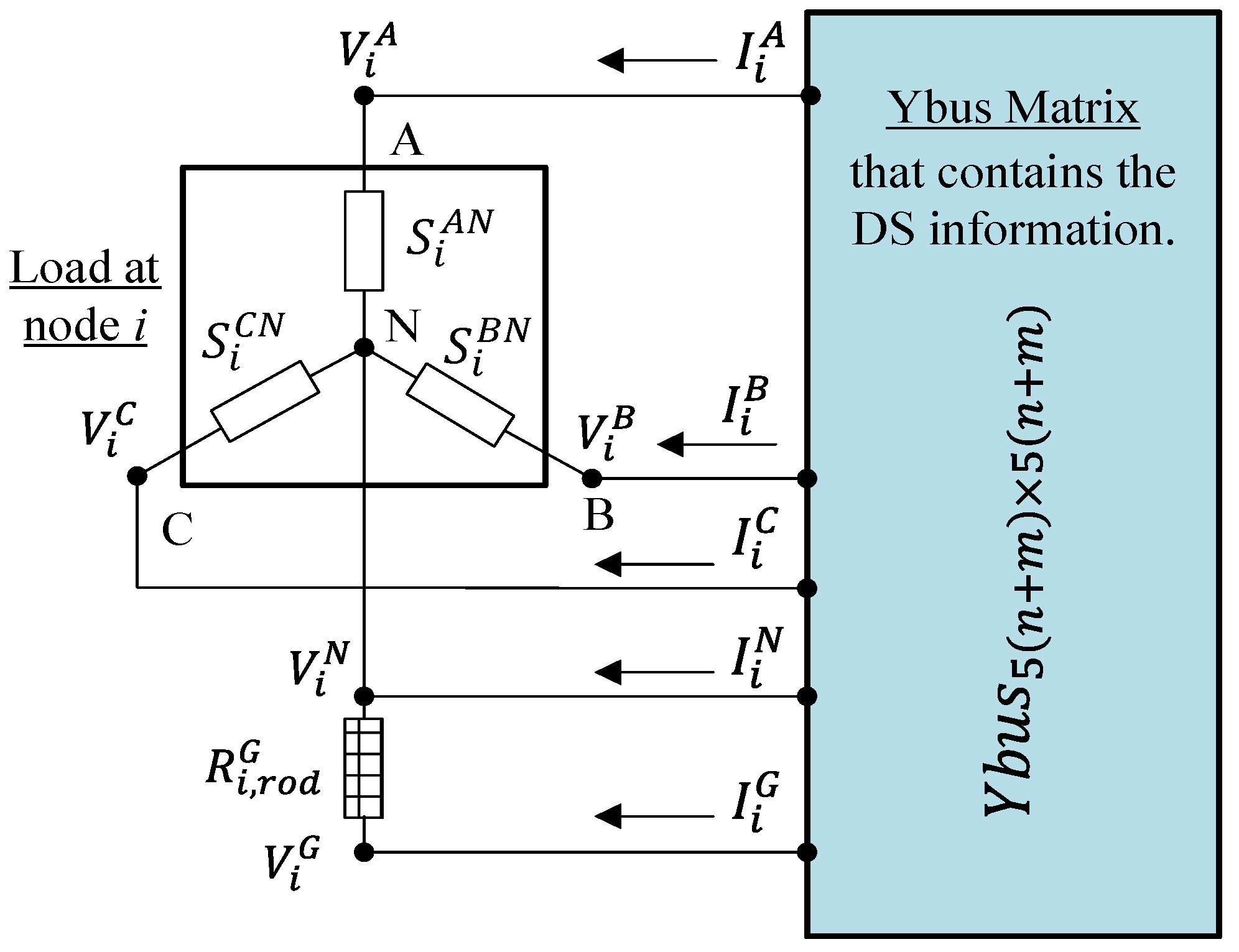
• A more accurate branch model is modified, which is in the 3 × 3 matrix deriving from the impedances of the phase-A, -B, -C, neutral, and ground conductors together with the grounding resistances.
• Improved LF equations are proposed for the application to the unbalanced DSs with both PQ and PV nodes where, at the PV nodes following [13,14], the voltage magnitude and phase angle of each phase are balanced and the sum of real power generation of each phase is constant.

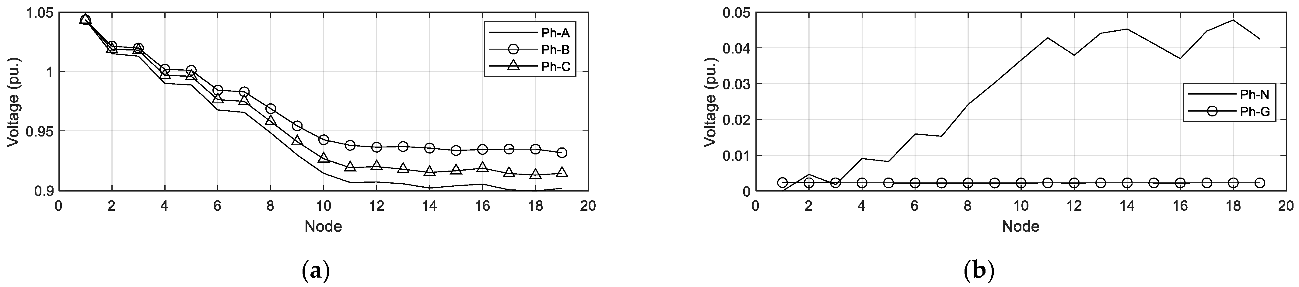
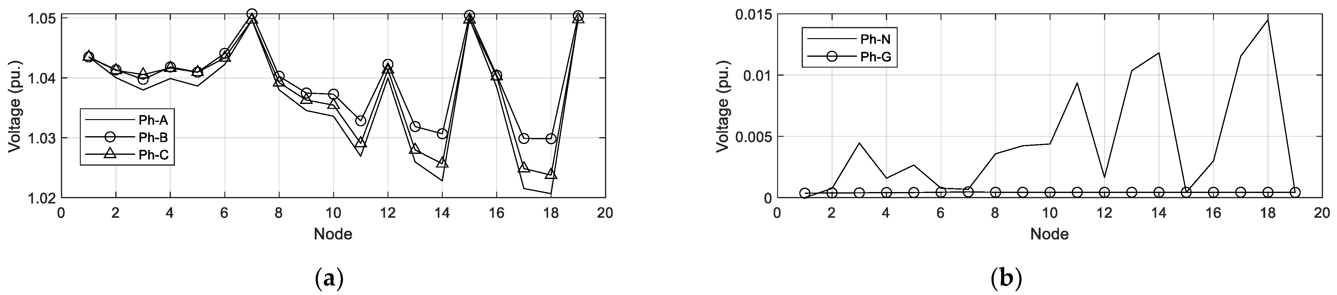
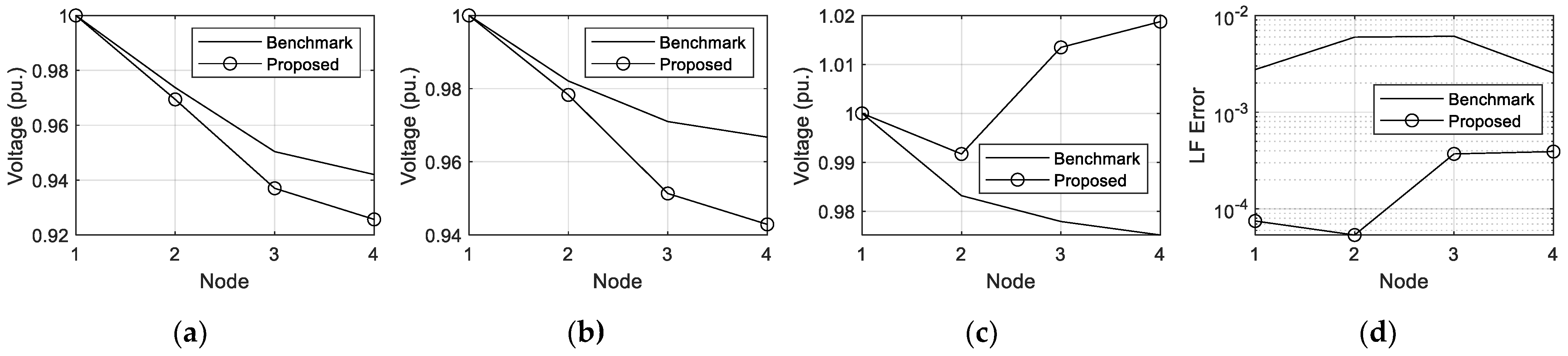
MATLAB is used for programming the NR method. Two unbalanced test LVDSs are demonstrated to validate the two proposed modifications. The simulation results of the modified branch model and the branch model simplified using Kron’s reduction will be compared and discussed.

In this paper, the simplified branch model, by using Kron’s reduction, and its disadvantages are described in Section 2. Section 3 proposes a modified branch model, which is in a 3 × 3 matrix derived from the impedances of the phase-A, -B, -C, neutral, and ground conductors together with the grounding resistances. The improved LF equations for the LVDSs with both PQ and PV nodes are also proposed in Section 3. Section 4 outlines and discusses numerical simulations. Finally, the conclusions of this paper are drawn in Section 5.

2. The Simplified Branch Model and Its Disadvantage

The original branch model with grounding resistances is shown in Figure 1 [3,6,15,16], where $S$ is load (VA); $R_G$ is grounding resistance (Ω); $V$ is voltage (V); $I$ is current (A); $z$ is the impedance in the branch model (Ω); $i$ and $j$ are any node in the LVDS; and $\left\{A,B,C,N,G\right\}$ is the set of phases in the branch model. From Figure 1, the branch equation can be written in two forms, as shown in Equations (1) and (2), in which direction is different, where $z_{ij}^{pq}=z_{ji}^{pq}$ following [3,6,15,16]; $p,q\in \left\{A,B,C,N,G\right\}$. The calculations of grounding resistance and branch impedances and the branch model simplified by using Kron’s reduction are described in Section 2.1, Section 2.2 and Section 2.3, respectively. Moreover, the disadvantage of using the simplified branch model can be clarified in Section 2.4.

$$\left[\begin{array}{c}{V}_i^A\\ V_i^B\\ V_i^C\\ V_i^N\\ V_i^G\end{array}\right]-\left[\begin{array}{c}{V}_j^A\\ V_j^B\\ V_j^C\\ V_j^N\\ V_j^G\end{array}\right]=\left[\begin{array}{ccccc}{z}_{ij}^{AA}& z_{ij}^{AB}& z_{ij}^{AC}& z_{ij}^{AN}& z_{ij}^{AG}\\ z_{ij}^{BA}& z_{ij}^{BB}& z_{ij}^{BC}& z_{ij}^{BN}& z_{ij}^{BG}\\ z_{ij}^{CA}& z_{ij}^{CB}& z_{ij}^{CC}& z_{ij}^{CN}& z_{ij}^{CG}\\ z_{ij}^{NA}& z_{ij}^{NB}& z_{ij}^{NC}& z_{ij}^{NN}& z_{ij}^{NG}\\ z_{ij}^{GA}& z_{ij}^{GB}& z_{ij}^{GC}& z_{ij}^{GN}& z_{ij}^{GG}\end{array}\right]\left[\begin{array}{c}{I}_{ij}^A\\ I_{ij}^B\\ I_{ij}^C\\ I_{ij}^N\\ I_{ij}^G\end{array}\right]$$

(1)

$$\left[\begin{array}{c}{V}_j^A\\ V_j^B\\ V_j^C\\ V_j^N\\ V_j^G\end{array}\right]-\left[\begin{array}{c}{V}_i^A\\ V_i^B\\ V_i^C\\ V_i^N\\ V_i^G\end{array}\right]=\left[\begin{array}{ccccc}{z}_{ji}^{AA}& z_{ji}^{AB}& z_{ji}^{AC}& z_{ji}^{AN}& z_{ji}^{AG}\\ z_{ji}^{BA}& z_{ji}^{BB}& z_{ji}^{BC}& z_{ji}^{BN}& z_{ji}^{BG}\\ z_{ji}^{CA}& z_{ji}^{CB}& z_{ji}^{CC}& z_{ji}^{CN}& z_{ji}^{CG}\\ z_{ji}^{NA}& z_{ji}^{NB}& z_{ji}^{NC}& z_{ji}^{NN}& z_{ji}^{NG}\\ z_{ji}^{GA}& z_{ji}^{GB}& z_{ji}^{GC}& z_{ji}^{GN}& z_{ji}^{GG}\end{array}\right]\left[\begin{array}{c}{I}_{ji}^A\\ I_{ji}^B\\ I_{ji}^C\\ I_{ji}^N\\ I_{ji}^G\end{array}\right]$$

(2)

Figure 1. The original branch model.

2.1. Grounding Resistance Calculation

Grounding systems of LVDSs must be designed to meet the requirement for reliable operation of connected electrical equipment, such as distributed generators and distribution transformers. The appropriate design of the grounding system can help in the following: (i) to prevent damage to insulation of connected electrical equipment; (ii) to ensure personal safety from touch and step voltages [2]. In many LVDSs, the grounding system uses cylindrical rods with each rod needing to have grounding resistance lower than 25 Ω following [17]. To assess the grounding resistance of each rod ($R_{rod}^G$), Equation (3) is used [2].

$$R_{rod}^G=\frac{{\rho }^G}{2·\pi ·l^{rod}}·ln\left(\frac{l^{rod}}{r{a}^{rod}}\right)$$

(3)

where ${\rho }^G$ is ground resistivity (Ω-m); $l^{rod}$ is length of the part of the cylindrical rod that is underground (m); and $r{a}^{rod}$ is the radius of the rod (m).

2.2. Branch Impedance Calculation

The resistance of each conductor ($R$) can be defined from the conductor datasheet, such as 185 mm² Weatherproof Aluminum Conductor (WAC) has $R$ of 0.2008 Ω/km [18]. For the branch impedances ($z$) in Equations (1) and (2), they can be calculated from the Carson’s equations with ground return, as shown in Equations (4)–(8) [5,6]. Note that Equations (4)–(8) are based on 50-Hz DSs.

$$z_{ij}^{GG}=0.0493+1j·0.3643$$

(4)

$$z_{ij}^{eG}=1j·0.01·\pi ·ln\left(\frac{d^{eG}}{\sqrt{0.02·{\rho }^G}}\right)$$

(5)

$$z_{ij}^{ee}=R_{ij}^{ee}+1j·0.02·\pi ·ln\left(\frac{2·d^{eG}}{GM{R}^e}\right)$$

(6)

$$z_{ij}^{ef}=1j·0.02·\pi ·ln\left[\frac{\sqrt{{\left(d^{ef}\right)}^2+{\left(d^{eG}+d^{fG}\right)}^2}}{\sqrt{{\left(d^{ef}\right)}^2+{\left(d^{eG}-d^{fG}\right)}^2}}\right]; e\ne f$$

(7)

$$GM{R}^e=0.7788·r{a}^e$$

(8)

where $z$ is in Ω/km; $1j$ is complex value; $e,f\in \left\{A,B,C,N\right\}$; $d^{eG}$ is height of phase-$e$ conductor (m); $GM{R}^e$ is geometric mean radius of phase-$e$ conductor (m); $d^{ef}$ is distance between phase-$e$ and phase-$f$ conductors (m); $r{a}^e$ is radius of phase-$e$ conductor (m).

2.3. The Branch Model Simplified by Using Kron’s Reduction

From Equation (1), when the voltages of neutral and ground conductors are simply defined as zero, Kron’s reduction can be used, and then Equation (1) is simplified into Equation (9) [16], where $z_{ij}^{r{s}^{\prime }}$ is the result of using Kron’s reduction; $r,s\in \left\{A,B,C\right\}$.

$$\left[\begin{array}{c}{V}_i^A\\ V_i^B\\ V_i^C\end{array}\right]-\left[\begin{array}{c}{V}_j^A\\ V_j^B\\ V_j^C\end{array}\right]=\left[\begin{array}{ccc}{z}_{ij}^{A{A}^{\prime }}& z_{ij}^{A{B}^{\prime }}& z_{ij}^{A{C}^{\prime }}\\ z_{ij}^{B{A}^{\prime }}& z_{ij}^{B{B}^{\prime }}& z_{ij}^{B{C}^{\prime }}\\ z_{ij}^{C{A}^{\prime }}& z_{ij}^{C{B}^{\prime }}& z_{ij}^{C{C}^{\prime }}\end{array}\right]\left[\begin{array}{c}{I}_{ij}^A\\ I_{ij}^B\\ I_{ij}^C\end{array}\right]$$

(9)

2.4. The Disadvantage of Using the Simplified Branch Model

The simplified branch model using Kron’s reduction is already stated in Section 2.3. The main problem of this model is that the neutral voltage is set to zero although load unbalance is varied. It contrasts with the load unbalance principle in [15] that the neutral voltage will be changed when load unbalance is varied. For the example, as shown in Figure 2a, when initial loads at phase A-N, B-N, and C-N of node $j$ ($S_j^{AN}$, $S_j^{BN}$, and $S_j^{CN}$) are $100+j50$, $100+j50$, and $200+j100$ W, respectively, the neutral voltage at node $j$ ($V_j^N$) is $0.57\angle {130.09}^{°}$ V. After increasing the load unbalance, if $S_j^{AN}$, $S_j^{BN}$, and $S_j^{CN}$ equal to $100+j50$, $100+j50$, and $3000+j1000$ W, respectively, $V_j^N$ is changed to $17.56\angle {135.92}^{°}$ V, as shown in Figure 2b. For another example, using Kron’s reduction in the circuit of Figure 2, the simplified circuit can be obtained in Figure 3. Load in Figure 3 is used the same as Figure 2, and then the voltage results can be marked in the figure. Both models of Figure 2 and Figure 3 will be compared with the phase-to-neutral voltage results, as shown in Table 1 where $V_j^{rN}=V_j^r-V_j^N$; $r\in \left\{A,B,C\right\}$. It can be noticed that the simplified branch model using Kron’s reduction causes more error on the phase-to-neutral voltage result when the load unbalance is increasing. It is because the simplified branch model determines fixed neutral voltage at zero.

Figure 2. The example of considering the full branch model in LF as: (a) when $S_j^{AN}$, $S_j^{BN}$, and $S_j^{CN}$ are $100+j50$, $100+j50$, and $200+j100$ W, respectively; (b) when $S_j^{AN}$, $S_j^{BN}$, and $S_j^{CN}$ are $100+j50$, $100+j50$, and $3000+j1000$ W, respectively.

Figure 3. The example of considering the simplified branch model in LF as: (a) when $S_j^{AN}$, $S_j^{BN}$, and $S_j^{CN}$ are $100+j50$, $100+j50$, and $200+j100$ W, respectively; (b) when $S_j^{AN}$, $S_j^{BN}$, and $S_j^{CN}$ are $100+j50$, $100+j50$, and $3000+j1000$ W, respectively.

Table 1. The comparison of the phase-to-neutral voltage results between the full and simplified branch models.

Phase-to-Neutral Voltage (V)	At the Initial			At Increasing Load Unbalance
	Full Model	Simplified Model	Voltage Error	Full Model	Simplified Model	Voltage Error
$V_j^{AN}$	230.04	229.83	−0.09%	242.61	229.83	−5.27%
$V_j^{BN}$	229.87	229.83	−0.02%	234.57	229.83	−2.02%
$V_j^{CN}$	228.78	229.65	0.38%	203.28	225.29	10.83%

3. Modified Branch Model and Improved LF Equations

Using the modified 4 × 4 branch model in the current injection NR method can suffer from the lack of convergence in the LVDSs with PV nodes [10]. Then, a modified 3 × 3 branch matrix is proposed in this paper for more convenience to modify the LF equations with PV nodes but with slight error. The error is due to the neglecting of the neutral and ground current injection from neighboring branches. Section 3.1 will clarify the derivation of the modified 3 × 3 branch matrix. After that, the improved LF equations with both PQ and PV nodes will be formulated in Section 3.2. The NR method for solving the improved LF equations will be clarified in Section 3.3. The LF result from the NR method is in the form of phase-to-neutral voltage. Following this, the voltages and currents of the neutral and ground conductors will be assessed in Section 3.4. Finally, the method for verifying the error of the LF results is explained in Section 3.5.

3.1. The Derivation of the Modified 3 × 3 Branch Matrix

The modified 3 × 3 branch matrix is derived from the impedances of the phase-A, -B, -C, neutral, and ground conductors together with the grounding resistances. To obtain this modified branch model, there are three processes, as indicated in Section 3.1.1, Section 3.1.2 and Section 3.1.3, and the relevant flowchart is shown in Figure 4. If a LVDS has many branches, the flowchart of formulating a Ybus matrix can be seen in Figure 5, where the Ybus matrix is the matrix that contains branch connections and impedance data of LVDS.

Figure 4. The flowchart of formulating the modified branch model.

Figure 5. The flowchart of Ybus formulation.

3.1.1. Finding Ground Current Equation

Initially, the ground current equation ($I_{ij}^G$) must be solved to reduce the original branch model into a 4 × 4 matrix in Section 4.2. Using matrix inversion for Equations (1) and (2), the following equations can be obtained, where $y_{ij}^{pq}=y_{ji}^{pq}$ according to [3,6,16]; $p,q\in \left\{A,B,C,N,G\right\}$.

$$\left[\begin{array}{c}{I}_{ij}^A\\ I_{ij}^B\\ I_{ij}^C\\ I_{ij}^N\\ I_{ij}^G\end{array}\right]=\left[\begin{array}{ccccc}{y}_{ij}^{AA}& y_{ij}^{AB}& y_{ij}^{AC}& y_{ij}^{AN}& y_{ij}^{AG}\\ y_{ij}^{BA}& y_{ij}^{BB}& y_{ij}^{BC}& y_{ij}^{BN}& y_{ij}^{BG}\\ y_{ij}^{CA}& y_{ij}^{CB}& y_{ij}^{CC}& y_{ij}^{CN}& y_{ij}^{CG}\\ y_{ij}^{NA}& y_{ij}^{NB}& y_{ij}^{NC}& y_{ij}^{NN}& y_{ij}^{NG}\\ y_{ij}^{GA}& y_{ij}^{GB}& y_{ij}^{GC}& y_{ij}^{GN}& y_{ij}^{GG}\end{array}\right]\left[\begin{array}{c}{V}_i^A-V_j^A\\ V_i^B-V_j^B\\ V_i^C-V_j^C\\ V_i^N-V_j^N\\ V_i^G-V_j^G\end{array}\right]$$

(10)

$$\left[\begin{array}{c}{I}_{ji}^A\\ I_{ji}^B\\ I_{ji}^C\\ I_{ji}^N\\ I_{ji}^G\end{array}\right]=\left[\begin{array}{ccccc}{y}_{ji}^{AA}& y_{ji}^{AB}& y_{ji}^{AC}& y_{ji}^{AN}& y_{ji}^{AG}\\ y_{ji}^{BA}& y_{ji}^{BB}& y_{ji}^{BC}& y_{ji}^{BN}& y_{ji}^{BG}\\ y_{ji}^{CA}& y_{ji}^{CB}& y_{ji}^{CC}& y_{ji}^{CN}& y_{ji}^{CG}\\ y_{ji}^{NA}& y_{ji}^{NB}& y_{ji}^{NC}& y_{ji}^{NN}& y_{ji}^{NG}\\ y_{ji}^{GA}& y_{ji}^{GB}& y_{ji}^{GC}& y_{ji}^{GN}& y_{ji}^{GG}\end{array}\right]\left[\begin{array}{c}{V}_j^A-V_i^A\\ V_j^B-V_i^B\\ V_j^C-V_i^C\\ V_j^N-V_i^N\\ V_j^G-V_i^G\end{array}\right]$$

(11)

The ground currents of Equations (10) and (11) are found using Equations (12) and (13). When Equation (12) is added to Equation (13), it can be proved that $I_{ij}^G=-I_{ji}^G$.

$$I_{ij}^G={\displaystyle \sum }_p\left[V_i^p-V_j^p\right]·y_{ij}^{Gp}$$

(12)

$$I_{ji}^G={\displaystyle \sum }_p\left[V_j^p-V_i^p\right]·y_{ji}^{Gp}$$

(13)

At Equation (1), the voltage equation at the ground conductor can be found using Equation (14). After that, $V_i^N$ is subtracted from Equation (14) and the result is divided by $R_{i,rod}^G$. Then, Equation (15) is obtained, where $I_{ij}^G=\left(V_i^G-V_i^N\right)/R_{i,rod}^G$ following Figure 1.

$$V_i^G-V_j^G={\displaystyle \sum }_p{z}_{ij}^{Gp}·I_{ij}^p$$

(14)

$$I_{ij}^G-\frac{V_j^G}{R_{i,rod}^G}=\left({\displaystyle \sum }_p\frac{z_{ij}^{Gp}·I_{ij}^p}{R_{i,rod}^G}\right)-\frac{V_i^N}{R_{i,rod}^G}$$

(15)

From Equation (1), the voltage at node $i$ phase $N$ is given in the following Equation (16), and then, by substituting Equation (16) into Equation (15), Equation (17) can be obtained.

$$V_i^N=\left({\displaystyle \sum }_p{z}_{ij}^{Np}·I_{ij}^p\right)+V_j^N$$

(16)

$$I_{ij}^G-\frac{V_j^G}{R_{i,rod}^G}=\left({\displaystyle \sum }_p\frac{z_{ij}^{Gp}·I_{ij}^p}{R_{i,rod}^G}\right)-\frac{\left({{\displaystyle \sum }}_p{z}_{ij}^{Np}·I_{ij}^p\right)+V_j^N}{R_{i,rod}^G}$$

(17)

Reformatting Equation (17) following $I_{ij}^G=-I_{ji}^G$ and $I_{ji}^G=\left(V_j^G-V_j^N\right)/R_{j,rod}^G$, the ground current equation ($I_{ij}^G$) is obtained in Equation (18), where $e\in \left\{A,B,C,N\right\}$.

$$I_{ij}^G-\frac{V_j^G}{R_{i,rod}^G}=\left({\displaystyle \sum }_p\frac{z_{ij}^{Gp}·I_{ij}^p}{R_{i,rod}^G}\right)-\frac{\left({{\displaystyle \sum }}_p{z}_{ij}^{Np}·I_{ij}^p\right)+V_j^N}{R_{i,rod}^G}$$

(18)

3.1.2. Formulating the Original Branch Model into the 4 × 4 Matrix

Equation (1) is reformulated into Equation (19) by neglecting the variables $V_i^G$ and $V_j^G$. Substituting $I_{ij}^G$ from Equation (18) into Equation (19), the branch matrix is then in a 4 × 4 matrix with vanishment of the variable $I_{ij}^G$, as written in Equation (20), where $k_{ij}^{ef}=z_{ij}^{ef}+\frac{z_{ij}^{eG}\left[z_{ij}^{Gf}-z_{ij}^{Nf}\right]}{R_{i,rod}^G+R_{j,rod}^G+z_{ij}^{NG}-z_{ij}^{GG}}$; $e,f\in \left\{A,B,C,N\right\}$.

$$\left[\begin{array}{c}{V}_i^A\\ V_i^B\\ V_i^C\\ V_i^N\end{array}\right]-\left[\begin{array}{c}{V}_j^A\\ V_j^B\\ V_j^C\\ V_j^N\end{array}\right]=\left[\begin{array}{cccc}{z}_{ij}^{AA}& z_{ij}^{AB}& z_{ij}^{AC}& z_{ij}^{AN}\\ z_{ij}^{BA}& z_{ij}^{BB}& z_{ij}^{BC}& z_{ij}^{BN}\\ z_{ij}^{CA}& z_{ij}^{CB}& z_{ij}^{CC}& z_{ij}^{CN}\\ z_{ij}^{NA}& z_{ij}^{NB}& z_{ij}^{NC}& z_{ij}^{NN}\end{array}\right]\left[\begin{array}{c}{I}_{ij}^A\\ I_{ij}^B\\ I_{ij}^C\\ I_{ij}^N\end{array}\right]+\left[\begin{array}{c}{z}_{ij}^{AG}\\ z_{ij}^{BG}\\ z_{ij}^{CG}\\ z_{ij}^{NG}\end{array}\right]I_{ij}^G$$

(19)

$$\left[\begin{array}{c}{V}_i^A\\ V_i^B\\ V_i^C\\ V_i^N\end{array}\right]-\left[\begin{array}{c}{V}_j^A\\ V_j^B\\ V_j^C\\ V_j^N\end{array}\right]=\left[\begin{array}{cccc}{k}_{ij}^{AA}& k_{ij}^{AB}& k_{ij}^{AC}& k_{ij}^{AN}\\ k_{ij}^{BA}& k_{ij}^{BB}& k_{ij}^{BC}& k_{ij}^{BN}\\ k_{ij}^{CA}& k_{ij}^{CB}& k_{ij}^{CC}& k_{ij}^{CN}\\ k_{ij}^{NA}& k_{ij}^{NB}& k_{ij}^{NC}& k_{ij}^{NN}\end{array}\right]·\left[\begin{array}{c}{I}_{ij}^A\\ I_{ij}^B\\ I_{ij}^C\\ I_{ij}^N\end{array}\right]$$

(20)

Equation (20) is reformulated into Equation (21) with $I_i^W=I_i^N+I_i^G$. To solve the variables $h_{ij}^{es}$ and $h_{ij}^{eW}$ in Equation (21), Equation (22) is formulated following the equality of Equations (20) and (21). The results of variables $h^{es}$ and $h^{eW}$ are shown in Table 2.

$$\left[\begin{array}{c}{V}_i^A\\ V_i^B\\ V_i^C\\ V_i^N\end{array}\right]-\left[\begin{array}{c}{V}_j^A\\ V_j^B\\ V_j^C\\ V_j^N\end{array}\right]=\left[\begin{array}{cccc}{h}_{ij}^{AA}& h_{ij}^{AB}& h_{ij}^{AC}& h_{ij}^{AW}\\ h_{ij}^{BA}& h_{ij}^{BB}& h_{ij}^{BC}& h_{ij}^{BW}\\ h_{ij}^{CA}& h_{ij}^{CB}& h_{ij}^{CC}& h_{ij}^{CW}\\ h_{ij}^{NA}& h_{ij}^{NB}& h_{ij}^{NC}& h_{ij}^{NW}\end{array}\right]·\left[\begin{array}{c}{I}_{ij}^A\\ I_{ij}^B\\ I_{ij}^C\\ I_{ij}^W\end{array}\right]$$

(21)

$$\left[\begin{array}{cccc}{k}_{ij}^{AA}& k_{ij}^{AB}& k_{ij}^{AC}& k_{ij}^{AN}\\ k_{ij}^{BA}& k_{ij}^{BB}& k_{ij}^{BC}& k_{ij}^{BN}\\ k_{ij}^{CA}& k_{ij}^{CB}& k_{ij}^{CC}& k_{ij}^{CN}\\ k_{ij}^{NA}& k_{ij}^{NB}& k_{ij}^{NC}& k_{ij}^{NN}\end{array}\right]·\left[\begin{array}{c}{I}_{ij}^A\\ I_{ij}^B\\ I_{ij}^C\\ I_{ij}^N\end{array}\right]=\left[\begin{array}{cccc}{h}_{ij}^{AA}& h_{ij}^{AB}& h_{ij}^{AC}& h_{ij}^{AW}\\ h_{ij}^{BA}& h_{ij}^{BB}& h_{ij}^{BC}& h_{ij}^{BW}\\ h_{ij}^{CA}& h_{ij}^{CB}& h_{ij}^{CC}& h_{ij}^{CW}\\ h_{ij}^{NA}& h_{ij}^{NB}& h_{ij}^{NC}& h_{ij}^{NW}\end{array}\right]·\left[\begin{array}{c}{I}_{ij}^A\\ I_{ij}^B\\ I_{ij}^C\\ I_{ij}^W\end{array}\right]$$

(22)

Table 2. Variable results from solving Equation (22).

Variable	Result
$h_{ij}^{eW}$	=	$\frac{z_{ij}^{eN}\left[R_{i,rod}^G+R_{j,rod}^G+z_{ij}^{NG}-z_{ij}^{GG}\right]+z_{ij}^{eG}\left[z_{ij}^{GN}-z_{ij}^{NN}\right]}{R_{i,rod}^G+R_{j,rod}^G+2z_{ij}^{NG}-z_{ij}^{NN}-z_{ij}^{GG}}$;
$h_{ij}^{es}$	=	$z_{ij}^{es}+\frac{\left[z_{ij}^{eG}-h_{ij}^{eW}\right]\left[z_{ij}^{Gs}-z_{ij}^{Ns}\right]}{R_{i,rod}^G+R_{j,rod}^G+z_{ij}^{NG}-z_{ij}^{GG}}$;
$e$	$\in$	$\left\{A,B,C,N\right\}$;
$s$	$\in$	$\left\{A,B,C\right\}.$

3.1.3. Obtaining the Modified Branch Model

The neutral voltage of Equation (21) is given in Equation (23), where $r\in \left\{A,B,C\right\}$. When Equation (21) has Equation (23) subtracted from it, Equation (24) can be obtained, where $V_i^{rN}=V_i^r-V_i^N$.

$$V_i^N-V_j^N=\left({\displaystyle \sum }_r{h}_{ij}^{Nr}·I_{ij}^r\right)+h_{ij}^{NW}{I}_{ij}^W$$

(23)

$$\left[\begin{array}{c}{V}_i^{AN}\\ V_i^{BN}\\ V_i^{CN}\end{array}\right]-\left[\begin{array}{c}{V}_j^{AN}\\ V_j^{BN}\\ V_j^{CN}\end{array}\right]=\left[\begin{array}{cccc}{h}_{ij}^{AA}& h_{ij}^{AB}& h_{ij}^{AC}& h_{ij}^{AW}\\ h_{ij}^{BA}& h_{ij}^{BB}& h_{ij}^{BC}& h_{ij}^{BW}\\ h_{ij}^{CA}& h_{ij}^{CB}& h_{ij}^{CC}& h_{ij}^{CW}\end{array}\right]\left[\begin{array}{c}{I}_{ij}^A\\ I_{ij}^B\\ I_{ij}^C\\ I_{ij}^W\end{array}\right]-\left[\begin{array}{cccc}{h}_{ij}^{NA}& h_{ij}^{NB}& h_{ij}^{NC}& h_{ij}^{NW}\\ h_{ij}^{NA}& h_{ij}^{NB}& h_{ij}^{NC}& h_{ij}^{NW}\\ h_{ij}^{NA}& h_{ij}^{NB}& h_{ij}^{NC}& h_{ij}^{NW}\end{array}\right]\left[\begin{array}{c}{I}_{ij}^A\\ I_{ij}^B\\ I_{ij}^C\\ I_{ij}^W\end{array}\right]$$

(24)

After that, Equation (24) is reformulated according to $I_{ij}^W=I_{ij}^N+I_{ij}^G=-\left(I_{ij}^A+I_{ij}^B+I_{ij}^C\right),$ and then the modified branch model is finally obtained as written in Equation (25), where $z_{ij}^{r{s}^{″}}=h_{ij}^{rs}-h_{ij}^{rW}-h_{ij}^{Ns}+h_{ij}^{NW}$; $r,s\in \left\{A,B,C\right\}$.

$$\left[\begin{array}{c}{V}_i^{AN}\\ V_i^{BN}\\ V_i^{CN}\end{array}\right]-\left[\begin{array}{c}{V}_j^{AN}\\ V_j^{BN}\\ V_j^{CN}\end{array}\right]=\left[\begin{array}{ccc}{z}_{ij}^{A{A}^{″}}& z_{ij}^{A{B}^{″}}& z_{ij}^{A{C}^{″}}\\ z_{ij}^{B{A}^{″}}& z_{ij}^{B{B}^{″}}& z_{ij}^{B{C}^{″}}\\ z_{ij}^{C{A}^{″}}& z_{ij}^{C{B}^{″}}& z_{ij}^{C{C}^{″}}\end{array}\right]\left[\begin{array}{c}{I}_{ij}^A\\ I_{ij}^B\\ I_{ij}^C\end{array}\right]$$

(25)

3.2. Formulating the Improved LF Equations

The improved LF equations, which include both PQ and PV nodes, can be seen in Equations (26)–(28), where reactive power injection at PV nodes is not determined because, at PV nodes, reactive power injections are not fixed during LF calculation using the NR method. The LF equation at PV nodes is presented in Equation (28) with total real power generation at PV node, node $i$ ($P_{i,PV}$), being constant [13,14]. Superscript $rN$ and $sN$ are used for overall Equations (26)–(28) due to the reference voltage being neutral, as expressed in Equation (25). Ybus matrix, applied in Equations (26)–(28), is formulated from the modified branch model in Equation (25). If a DS includes one slack node, $n-1$ PQ nodes, and $m$ PV nodes, the $Ybus$ is in the $3\left(n+m\right)\times 3\left(n+m\right)$ matrix.

$$\begin{array}{c}{P}_{i,PQ}^{rN}={\displaystyle {\displaystyle \sum }_s}|V_{i,PQ}^{rN}||V_1^{sN}||Y_{i1}^{rs}|cos({\theta }_{i1}^{rs}-{\delta }_{i,PQ}^{rN}+{\delta }_1^{sN})+{\displaystyle {\displaystyle \sum }_{j=2}^n{\displaystyle \sum }_s}|V_{i,PQ}^{rN}||V_{j,PQ}^{sN}||Y_{i\mathrm{j}}^{rs}|cos({\theta }_{i\mathrm{j}}^{rs}-{\delta }_{i,PQ}^{rN}+{\delta }_{j,PQ}^{sN})\\ +{\displaystyle {\displaystyle \sum }_{j=n+1}^{n+m}{\displaystyle \sum }_s}|V_{i,PQ}^{rN}||V_{j,PV}^{sN}||Y_{i\mathrm{j}}^{rs}|cos({\theta }_{i\mathrm{j}}^{rs}-{\delta }_{i,PQ}^{rN}+{\delta }_{j,PV}^{AN}+{\mu }_{j,PV}^{sN})\end{array}$$

(26)

$$\begin{array}{c}{Q}_{i,PQ}^{rN}={\displaystyle {\displaystyle \sum }_s}|V_{i,PQ}^{rN}||V_1^{sN}||Y_{i1}^{rs}|sin({\theta }_{i1}^{rs}-{\delta }_{i,PQ}^{rN}+{\delta }_1^{sN})-{\displaystyle {\displaystyle \sum }_{j=2}^n{\displaystyle \sum }_s}|V_{i,PQ}^{rN}||V_{j,PQ}^{sN}||Y_{i\mathrm{j}}^{rs}|sin({\theta }_{i\mathrm{j}}^{rs}-{\delta }_{i,PQ}^{rN}+{\delta }_{j,PQ}^{sN})\\ -{\displaystyle {\displaystyle \sum }_{j=n+1}^{n+m}{\displaystyle \sum }_s}|V_{i,PQ}^{rN}||V_{j,PV}^{sN}||Y_{i\mathrm{j}}^{rs}|sin({\theta }_{i\mathrm{j}}^{rs}-{\delta }_{i,PQ}^{rN}+{\delta }_{j,PV}^{AN}+{\mu }_{j,PV}^{sN})\end{array}$$

(27)

$$P_{i,PV}={\displaystyle \sum }_r{P}_{i,PV}^{rN}-{\displaystyle \sum }_r{P}_{i,load}^{rN}$$

(28)

$$\begin{array}{c}{P}_{i,PV}^{rN}={\displaystyle {\displaystyle \sum }_s}|V_{i,PQ}^{rN}||V_1^{sN}||Y_{i1}^{rs}|cos({\theta }_{i1}^{rs}-{\delta }_{i,PV}^{AN}-{\mu }_{i,PV}^{rN}+{\delta }_1^{sN})+{\displaystyle {\displaystyle \sum }_{j=2}^n{\displaystyle \sum }_s}|V_{i,PV}^{rN}||V_{j,PQ}^{sN}||Y_{i\mathrm{j}}^{rs}|cos({\theta }_{i\mathrm{j}}^{rs}-{\delta }_{i,PV}^{AN}-{\mu }_{i,PV}^{rN}+{\delta }_{j,PQ}^{sN})\\ -{\displaystyle {\displaystyle \sum }_{j=n+1}^{n+m}{\displaystyle \sum }_s}|V_{i,PV}^{rN}||V_{j,PV}^{sN}||Y_{i\mathrm{j}}^{rs}|cos({\theta }_{i\mathrm{j}}^{rs}-{\delta }_{i,PV}^{AN}-{\mu }_{j,PV}^{rN}+{\delta }_{i,PV}^{AN}+{\mu }_{j,PV}^{sN})\end{array}$$

(29)

where $P_{i,PV}$ is the sum of real power generation of each phase at PV node, node $i$ (W); $P_{i,PV}^{rN}$ is real power injection at PV node, node $i$, and phase $rN$ (W); $P_{i,load}^{rN}$ is specified load, connected at node $i$, and phase $rN$ (W); $r,s\in \left\{A,B,C\right\}$; $|Y_{ij}^{rs}|\angle {\theta }_{ij}^{rs}, |Y_{i1}^{rs}|\angle {\theta }_{i1}^{rs}\in Ybu{s}_{3\left(n+m\right)\times 3\left(n+m\right)}$; ${\mu }_{i,PV}^{AN}$, ${\mu }_{i,PV}^{BN}$, and ${\mu }_{i,PV}^{CN}$ equal to zero, −120°, and 120°, respectively. Note that, in Equations (26)–(28), ${\delta }_{i,PV}^{AN}+{\mu }_{i,PV}^{rN}$ and ${\delta }_{j,PV}^{AN}+{\mu }_{j,PV}^{sN}$ actually equal to ${\delta }_{i,PV}^{rN}$ and ${\delta }_{j,PV}^{sN}$, respectively. For the reason why Equations (26)–(28) are written in the form of ${\delta }_{i,PV}^{AN}$ or ${\delta }_{j,PV}^{AN}$, it is because phase angle at PV node is balanced and then only ${\delta }_{i,PV}^{AN}$ or ${\delta }_{j,PV}^{AN}$ is used for calculation in the NR method.

To solve these improved LF equations, the NR method is applied as detailed in Section 3.3. The LF result from Section 3.3 is in the form of phase-to-neutral voltage. Following this, the voltages and currents of neutral and ground conductors will be assessed in Section 3.4. Finally, the method for verifying the error of LF results is explained in Section 3.5.

3.3. Solving the Improved LF Equations by the NR Method

In this section, Equations (26)–(28) are reformulated into the set of linear equations, as shown in Equation (30), by expanding them into the Taylor’s series and leaving all higher order terms. Each variable of Equation (30) is explained in Table 3. Following the conceptual calculation of the NR method [15], Equation (30) will be iteratively calculated, and voltage magnitudes and phase angles will be updated until the criteria in both Equations (31) and (32) are satisfied. The relevant flowchart of solving the improved LF equations by the NR method can be seen in Figure 6, where the superscripts of $sch$ and $cal$ mean the defined and calculated values, respectively; $t$ is iteration number.

$$\left[\begin{array}{c}\Delta P{Q}_{2,PQ}^{ABC-N}\\ \Delta P{Q}_{3,PQ}^{ABC-N}\\ ⋮\\ \Delta P{Q}_{n,PQ}^{ABC-N}\\ ---\\ \Delta P_{n+1,PV}\\ \Delta P_{n+2,PV}\\ ⋮\\ \Delta P_{n+m,PV}\end{array}\right]=\left[\begin{array}{ccc}\begin{array}{cc}\begin{array}{cc}{J}_{2,2}& J_{2,3}\\ J_{3,2}& J_{3,3}\end{array}& \begin{array}{cc}\cdots & J_{2,n}\\ \cdots & J_{3,n}\end{array}\\ \begin{array}{cc}⋮& ⋮\\ J_{n,2}& J_{n,3}\end{array}& \begin{array}{cc}\ddots & ⋮\\ \cdots & J_{n,n}\end{array}\end{array}& \begin{array}{c}\begin{array}{c}|\\ |\end{array}\\ \begin{array}{c}|\\ |\end{array}\end{array}& \begin{array}{cc}\begin{array}{cc}{E}_{2,n+1}& E_{2,n+2}\\ E_{3,n+1}& E_{3,n+2}\end{array}& \begin{array}{cc}\cdots & E_{2,n+m}\\ \cdots & E_{3,n+m}\end{array}\\ \begin{array}{cc}⋮& ⋮\\ E_{n,n+1}& E_{n,n+2}\end{array}& \begin{array}{cc}\ddots & ⋮\\ \cdots & E_{n,n+m}\end{array}\end{array}\\ \begin{array}{cc}\begin{array}{ccc}-& -& -\end{array}& \begin{array}{ccc}-& -& \begin{array}{cc}-& -\end{array}\end{array}\end{array}& +& \begin{array}{cc}\begin{array}{ccc}-& -& -\end{array}& \begin{array}{ccc}-& -& \begin{array}{cc}-& -\end{array}\end{array}\end{array}\\ \begin{array}{cc}\begin{array}{cc}{F}_{n+1,2}& F_{n+1,3}\\ F_{n+2,2}& F_{n+2,3}\end{array}& \begin{array}{cc}\cdots & F_{n+1,n}\\ \cdots & F_{n+2,n}\end{array}\\ \begin{array}{cc}⋮& ⋮\\ F_{n+m,2}& F_{n+m,3}\end{array}& \begin{array}{cc}\ddots & ⋮\\ \cdots & F_{n+m,n}\end{array}\end{array}& \begin{array}{c}\begin{array}{c}|\\ |\end{array}\\ \begin{array}{c}|\\ |\end{array}\end{array}& \begin{array}{cc}\begin{array}{cc}{K}_{n+1,n+1}& K_{n+1,n+2}\\ K_{n+2,n+1}& K_{n+2,n+2}\end{array}& \begin{array}{cc}\cdots & K_{n+1,n+m}\\ \cdots & K_{n+2,n+m}\end{array}\\ \begin{array}{cc}⋮& ⋮\\ K_{n+m,n+1}& K_{n+m,n+2}\end{array}& \begin{array}{cc}\ddots & ⋮\\ \cdots & K_{n+m,n+m}\end{array}\end{array}\end{array}\right]\left[\begin{array}{c}\Delta |V|{\delta }_{2,PQ}^{ABC-N}\\ \Delta |V|{\delta }_{3,PQ}^{ABC-N}\\ ⋮\\ \Delta |V|{\delta }_{n,PQ}^{ABC-N}\\ ---\\ \Delta {\delta }_{n+1,PV}^{AN}\\ \Delta {\delta }_{n+2,PV}^{AN}\\ ⋮\\ \Delta {\delta }_{n+m,PV}^{AN}\end{array}\right]$$

(30)

$$\underset{i\in \left\{PQ nodes\right\}}{\max }\left(|\Delta P_{i,PQ}^{rN}|,|\Delta Q_{i,PQ}^{rN}|\right)\le \epsilon$$

(31)

$$\underset{i\in \left\{PV nodes\right\}}{\max }\left(|\Delta P_{i,PV}|\right)\le \epsilon$$

(32)

Table 3. Meaning of variables in Equations (30).

Variable	Meaning
$\Delta P{Q}_{i,PQ}^{ABC-N}$	$=$	${\left[\begin{array}{cc}\Delta P_{i,PQ}^{ABC-N}& \Delta Q_{i,PQ}^{ABC-N}\end{array}\right]}^T$;
$\Delta |V|{\delta }_{i,PQ}^{ABC-N}$	$=$	${\left[\begin{array}{cc}\Delta |V_{i,PQ}^{ABC-N}|& \Delta {\delta }_{i,PQ}^{ABC-N}\end{array}\right]}^T$;
$\Delta P_{i,PQ}^{ABC-N}$	$=$	$\left[\begin{array}{ccc}\Delta P_{i,PQ}^{AN}& \Delta P_{i,PQ}^{BN}& \Delta P_{i,PQ}^{CN}\end{array}\right]$;
$\Delta Q_{i,PQ}^{ABC-N}$	$=$	$\left[\begin{array}{ccc}\Delta Q_{i,PQ}^{AN}& \Delta Q_{i,PQ}^{BN}& \Delta Q_{i,PQ}^{CN}\end{array}\right]$;
$\Delta |V_{i,PQ}^{ABC-N}|$	$=$	$\left[\begin{array}{ccc}\Delta |V_{i,PQ}^{AN}|& \Delta |V_{i,PQ}^{BN}|& \Delta |V_{i,PQ}^{CN}|\end{array}\right]$;
$\Delta {\delta }_{i,PQ}^{ABC-N}$	$=$	$\left[\begin{array}{ccc}\Delta {\delta }_{i,PQ}^{AN}& \Delta {\delta }_{i,PQ}^{BN}& \Delta {\delta }_{i,PQ}^{CN}\end{array}\right]$;
$J,E,F,\mathrm{and}K$	are	Jacobian matrix.

Figure 6. The flowchart of solving the improved LF equations by the NR method.

3.4. Voltage and Currents Assessment at Neutral and Ground Conductors

Phase-to-neutral voltage magnitudes are obtained from solving the LF equations, and the modified branch model in Equation (25) does not reveal the existence of the voltages and currents of neutral and ground conductors. Then, these values are assessed in this section through the following four steps.

STEP 1: After solving the improved LF equations with the NR method and receiving the results of phase-to-neutral voltage ($V_i^{rN}$), the current sum ($I_{ij}^W$) of each branch is calculated in Equation (34).

$$\left[\begin{array}{c}{I}_{ij}^A\\ I_{ij}^B\\ I_{ij}^C\end{array}\right]=\left[\begin{array}{ccc}{y}_{ij}^{A{A}^{″}}& y_{ij}^{A{B}^{″}}& y_{ij}^{A{C}^{″}}\\ y_{ij}^{B{A}^{″}}& y_{ij}^{B{B}^{″}}& y_{ij}^{B{C}^{″}}\\ y_{ij}^{C{A}^{″}}& y_{ij}^{C{B}^{″}}& y_{ij}^{C{C}^{″}}\end{array}\right]·\left[\begin{array}{c}{V}_i^{AN}-V_j^{AN}\\ V_i^{BN}-V_j^{BN}\\ V_i^{CN}-V_j^{CN}\end{array}\right]$$

(33)

$$I_{ij}^W=-\left(I_{ij}^A+I_{ij}^B+I_{ij}^C\right)=I_{ij}^N+I_{ij}^G$$

(34)

STEP 2: After calculating $I_{ij}^W$, the currents of neutral and ground conductors ($I_{ij}^N$ and $I_{ij}^G$) need to be calculated. Following Equation (18), both sides of the equation have $I_{ij}^N$ subtracted from them. After that, the term $I_{ij}^N+I_{ij}^G$ is reformulated into $I_{ij}^W$, then Equation (35) is used to calculate $I_{ij}^N$, where $r\in \left\{A,B,C\right\}$. When $I_{ij}^N$ is known, Equation (36) can be used to calculate $I_{ij}^G$.

$$I_{ij}^N=\frac{\left[R_{i,rod}^G+R_{j,rod}^G+z_{ij}^{NG}-z_{ij}^{GG}\right]I_{ij}^W-{{\displaystyle \sum }}_r\left[z_{ij}^{Gr}-z_{ij}^{Nr}\right]I_{ij}^r}{R_{i,rod}^G+R_{j,rod}^G+2z_{ij}^{NG}-z_{ij}^{NN}-z_{ij}^{GG}}$$

(35)

$$I_{ij}^G=I_{ij}^W-I_{ij}^N$$

(36)

STEP 3: When all phase currents of each branch are known, the neutral and ground voltages ($V_1^N$ and $V_1^G$) at the slack or first node must be found. However, $V_1^N$ is generally defined as zero [3,16]. Following this, $V_1^G$ can be found in Equation (37), which is derived from the ground current following Figure 1, assuming that $i$ is the node adjacent to the slack node.

$$V_1^G=I_{1i}^G·R_{1,rod}^G$$

(37)

STEP 4: When the voltages at the first node are known, the voltages at node $i$, or the node adjacent to the slack node, can be calculated from Equation (38).

$$\left[\begin{array}{c}{V}_i^A\\ V_i^B\\ V_i^C\\ V_i^N\\ V_i^G\end{array}\right]=\left[\begin{array}{c}{V}_1^A\\ V_1^B\\ V_1^C\\ V_1^N\\ V_1^G\end{array}\right]-\left[\begin{array}{ccccc}{z}_{1i}^{AA}& z_{1i}^{AB}& z_{1i}^{AC}& z_{1i}^{AN}& z_{1i}^{AG}\\ z_{1i}^{BA}& z_{1i}^{BB}& z_{1i}^{BC}& z_{1i}^{BN}& z_{1i}^{BG}\\ z_{1i}^{CA}& z_{1i}^{CB}& z_{1i}^{CC}& z_{1i}^{CN}& z_{1i}^{CG}\\ z_{1i}^{NA}& z_{1i}^{NB}& z_{1i}^{NC}& z_{1i}^{NN}& z_{1i}^{NG}\\ z_{1i}^{GA}& z_{1i}^{GB}& z_{1i}^{GC}& z_{1i}^{GN}& z_{1i}^{GG}\end{array}\right]\left[\begin{array}{c}{I}_{1i}^A\\ I_{1i}^B\\ I_{1i}^C\\ I_{1i}^N\\ I_{1i}^G\end{array}\right]$$

(38)

STEP 5: The voltages at node $j$ can be calculated from Equation (39) assuming that $j$ is the node adjacent to node $i$. The voltages at node $i$ are known from the calculation in STEP 4. All members of $j$ or $\left\{2,3,\dots ,n,n+1,\dots ,n+m\right\}$ will be selected to accomplish the voltage and current assessments of overall neutral and ground conductors. The result of voltage assessments is shown in the form of phase separation in Equation (40), where $V_{1,slack}^N=0$ V. The subscript of $res$ means the result value from the assessment.

$$\left[\begin{array}{c}{V}_j^A\\ V_j^B\\ V_j^C\\ V_j^N\\ V_j^G\end{array}\right]=\left[\begin{array}{c}{V}_i^A\\ V_i^B\\ V_i^C\\ V_i^N\\ V_i^G\end{array}\right]-\left[\begin{array}{ccccc}{z}_{ij}^{AA}& z_{ij}^{AB}& z_{ij}^{AC}& z_{ij}^{AN}& z_{ij}^{AG}\\ z_{ij}^{BA}& z_{ij}^{BB}& z_{ij}^{BC}& z_{ij}^{BN}& z_{ij}^{BG}\\ z_{ij}^{CA}& z_{ij}^{CB}& z_{ij}^{CC}& z_{ij}^{CN}& z_{ij}^{CG}\\ z_{ij}^{NA}& z_{ij}^{NB}& z_{ij}^{NC}& z_{ij}^{NN}& z_{ij}^{NG}\\ z_{ij}^{GA}& z_{ij}^{GB}& z_{ij}^{GC}& z_{ij}^{GN}& z_{ij}^{GG}\end{array}\right]\left[\begin{array}{c}{I}_{ij}^A\\ I_{ij}^B\\ I_{ij}^C\\ I_{ij}^N\\ I_{ij}^G\end{array}\right]$$

(39)

3.5. The Error Assessment from LF Results

This section formulates the Ybus matrix from the original branch model in Equation (1), which results in a $5\left(n+m\right)\times 5\left(n+m\right)$ matrix. As determined at any node $i$ shown in Figure 7, the error ($er{r}_i$) can be calculated from the current summation in Equation (41). If there is no error from LF results, the current summation must be zero.

$$\left[\begin{array}{c}{V}_{1,slack,res}\\ V_{2,PQ,res}\\ ⋮\\ V_{n,PQ,res}\\ V_{n+1,PV,res}\\ ⋮\\ V_{n+m,PV,res}\end{array}\right]=\left[\begin{array}{lllll}{V}_{1,slack,res}^A& V_{1,slack,res}^B& V_{1,slack,res}^C& V_{1,slack,res}^N& V_{1,slack,res}^G\\ V_{2,PQ,res}^A& V_{2,PQ,res}^B& V_{2,PQ,res}^C& V_{2,PQ,res}^N& V_{2,PQ,res}^G\\ & & ⋮& & \\ V_{n,PQ,res}^A& V_{n,PQ,res}^B& V_{n,PQ,res}^C& V_{n,PQ,res}^N& V_{n,PQ,res}^G\\ V_{n+1,PV,res}^A& V_{n+1,PV,res}^B& V_{n+1,PV,res}^C& V_{n+1,PV,res}^N& V_{n+1,PV,res}^G\\ & & ⋮& & \\ V_{n+m,PV,res}^A& V_{n+m,PV,res}^B& V_{n+m,PV,res}^C& V_{n+m,PV,res}^N& V_{n+m,PV,res}^G\end{array}\right]$$

(40)

$$er{r}_i=\left|{\displaystyle \sum }_p{I}_i^p\right|=\left|{\displaystyle \sum }_{j=1}^{n+m}{\displaystyle \sum }_p{\displaystyle \sum }_q{Y}_{ij}^{pq}·V_{j,res}^q\right|$$

(41)

where $p,q\in \left\{A,B,C,N,G\right\}$; $Y_{ij}^{pq}\in Ybu{s}_{5\left(n+m\right)\times 5\left(n+m\right)}$ and is in pu.; $V_{j,res}$ is the voltage result (pu.) in the complex form at node $j$ obtained from the voltage and current assessments in Section 3.4, or expressed in Equation (40).

Figure 7. Node $i$ in Ybus matrix that is separated into phase-A, -B, -C, -N, and -G.

4. Simulation Results and Discussion

In this paper, MATLAB is used on a computer with AMD Ryzen5 2500U, 2.00 GHz, and 8 GB of RAM. To show the effectiveness of the modified branch model and improved LF equations, the two following methods are used for comparison.

• Benchmark Method: This traditional method is widely used for power flow comparison [7,8,11,15,16]. This method is the NR method based on the polar-form power injection approach. However, a branch model is simplified by defining the neutral and ground voltages as zero and then using Kron’s reduction to transform into a 3 × 3 branch matrix. Following this, the voltage result from this method is included in Equation (42), which will be used for the error assessment, as stated in Section 3.5, such that the values of $V_i^N$ and $V_i^G$ equal zero.
• Proposed method: The NR method is used for solving the improved LF equations, and the modified branch model is also applied. This method is proposed as stated in Section 3.

In this paper, the physical and configuration parameters of the conductors applied for the 4- and 19-node LVDSs are clarified in Appendix A. The connection node and load details of the 4- and 19-node LVDSs are demonstrated as detailed in Appendix B and Appendix C, respectively. To show the effectiveness of the proposed method, the simulation results are divided into four parts for performing the LF calculations between the proposed and benchmark methods on (i) 4-node LVDS with only PQ nodes, (ii) 19-node LVDS with only PQ nodes, (iii) 4-node LVDS with both PQ and PV nodes, and (iv) 19-node LVDS with both PQ and PV nodes. For both the 4- and 19-node LVDSs, the base voltage and base power are 230 V and 1 MVA, respectively.

$$\left[\begin{array}{c}{V}_{1,slack,res}\\ V_{2,PQ,res}\\ ⋮\\ V_{n,PQ,res}\\ V_{n+1,PV,res}\\ ⋮\\ V_{n+m,PV,res}\end{array}\right]=\left[\begin{array}{lllll}{V}_{1,slack,res}^A& V_{1,slack,res}^B& V_{1,slack,res}^C& 0& 0\\ V_{2,PQ,res}^A& V_{2,PQ,res}^B& V_{2,PQ,res}^C& 0& 0\\ & & ⋮& & \\ V_{n,PQ,res}^A& V_{n,PQ,res}^B& V_{n,PQ,res}^C& 0& 0\\ V_{n+1,PV,res}^A& V_{n+1,PV,res}^B& V_{n+1,PV,res}^C& 0& 0\\ & & ⋮& & \\ V_{n+m,PV,res}^A& V_{n+m,PV,res}^B& V_{n+m,PV,res}^C& 0& 0\end{array}\right]$$

(42)

4.1. Performing LF Calculation on 4-Nodes LVDS with Only PQ Nodes

In this section, both the benchmark and proposed methods converge in four iterations and at around 0.11 s. The phase voltage results of the proposed methods, from the voltage and current assessments as stated in Section 3.5, are shown in Figure 8. The comparisons of the phase-to-neutral voltages together with the errors in the LF results between the benchmark and proposed methods are shown in Figure 9. Note that the neutral voltages in the benchmark methods are equal to zero.

Figure 8. Phase voltage results of (a) Phase-A, -B, and -C and (b) Phase-N and -G.

Figure 9. Comparison between benchmark and proposed methods at (a) Phase-AN, (b) Phase-BN, (c) Phase-CN, and (d) errors in LF results.

From Figure 9, the phase-to-neutral voltages of the benchmark and proposed methods differ by around 0–0.04 pu., and the proposed method has around ten times less error than the benchmark method.

4.2. Performing LF Calculation on 19-Nodes LVDS with Only PQ Nodes

Both the benchmark and proposed methods converge in four iterations and at around 0.40 s. The phase voltage results of the proposed method, from the voltage and current assessments as stated in Section 3.5, are shown in Figure 10. The comparisons of the phase-to-neutral voltages together with the errors in the LF results between the benchmark and proposed methods are shown in Figure 11.

Figure 10. Phase voltage results of (a) Phase-A, -B, and -C and (b) Phase-N and -G.

Figure 11. Comparison between benchmark and proposed methods at (a) Phase-AN, (b) Phase-BN, (c) Phase-CN, and (d) errors in LF results.

From Figure 11, the phase-to-neutral voltages of the benchmark and proposed methods differ by around 0–0.04 pu., and the proposed method has around ten times less error than the benchmark method.

4.3. Performing LF Calculation on 4-Nodes LVDS with Both PQ and PV Nodes

In this section, node 4 is defined as a PV node and detailed in Table 4, where $r\in \left\{A,B,C\right\}$. Note that, at the PV node in this paper, the voltage magnitude and phase angle of each phase are balanced and the sum of real power generation of each phase ($P_{i,PV}$) is constant. The meaning of the balanced phase angle is ${\delta }_{i,PV}^{BN}={\delta }_{i,PV}^{AN}+{\mu }_{i,PV}^{BN}$ and ${\delta }_{i,PV}^{CN}={\delta }_{i,PV}^{AN}+{\mu }_{i,PV}^{CN}$, as already written in Equations (32)–(34).

Table 4. The details of PV node.

Node	${\mathit{P}}_{\mathit{i},\mathit{P}\mathit{V}}$ (W)	${\mathit{V}}_{\mathit{i}}^{\mathit{r}\mathit{N}}$ (pu.)
4	10,000	1

Performing the LF calculation in this section, both the benchmark and proposed methods converge in three iterations at around 0.10 s. The phase voltage results of the proposed method, from the voltage and current assessments as stated in Section 3.5, are shown in Figure 12. The power generation at the PV node of the benchmark and proposed methods is shown in Table 5. The comparisons of the phase-to-neutral voltages together with the errors in the LF results between the benchmark and proposed methods are shown in Figure 13.

Figure 12. Phase voltage results of (a) Phase-A, -B, and -C and (b) Phase-N and -G.

Table 5. Power generation at the PV node of benchmark and proposed methods.

Method	Node	Power Generation (VA)
		Phase AN	Phase BN	Phase CN
Benchmark	4	6725 + j16,109	3592 + j16,168	−316 + j13,076
Proposed	4	6614 + j15,976	3540 + j16,364	−153 + j13,016

Figure 13. Comparison between benchmark and proposed methods at (a) Phase-AN, (b) Phase-BN, (c) Phase-CN, and (d) errors in LF results.

As shown in Table 5, the results of the power generation at the PV node from the benchmark and proposed methods are close. From Figure 13, the phase-to-neutral voltages of the benchmark and proposed methods differ by around 0–0.01 pu., and the proposed method has around ten times less error than the benchmark method.

4.4. Performing LF Calculation on 19-Nodes LVDS with Both PQ and PV Nodes

In this section, nodes 7, 15, and 19 are defined as PV nodes and detailed in Table 6. In the LF calculations, both the benchmark and proposed methods converge in four iterations at around 0.40 s. The phase voltage results of the proposed methods, from the voltage and current assessments as stated in Section 3.5, are shown in Figure 14. The power generation at the PV nodes of the benchmark and proposed methods is shown in Table 7. The comparisons of the phase-to-neutral voltages together with the errors in the LF results between the benchmark and proposed methods are shown in Figure 15.

Table 6. The details of PV nodes.

Node	${\mathit{P}}_{\mathit{i},\mathit{P}\mathit{V}}$ (W)	${\mathit{V}}_{\mathit{i}}^{\mathit{r}\mathit{N}}$ (pu.)
7	70,000	1.05
15	150,000	1.05
19	50,000	1.05

Figure 14. Phase voltage results of (a) Phase-A, -B, and -C and (b) Phase-N and -G.

Table 7. Power generation at PV nodes of benchmark and proposed methods.

Method	Node	Power Generation (VA)
		Phase AN	Phase BN	Phase CN
Benchmark	7	27,230 + j41,658	22,205 + j42,826	20,565 + j41,005
	15	49,042 + j30,012	47,961 + j30,013	52,997 + j32,580
	19	14,632 − j1157	16,845 − j1071	18,523 + j529
Proposed	7	26,853 + j41,599	22,158 + j43,083	20,990 + j40,792
	15	48,821 + j30,262	47,824 + j29,889	53,355 + j32,572
	19	14,713 − j1078	16,874 − j1170	18,413 + j570

Figure 15. Comparison between benchmark and proposed methods at (a) Phase-AN, (b) Phase-BN, (c) Phase-CN, and (d) errors in LF results.

As shown in Table 7, the results of the power generation at the PV nodes from the benchmark and proposed methods are close. From Figure 15, the phase-to-neutral voltages of the benchmark and proposed methods differ by around 0–0.01 pu., and the proposed method has around ten times less error than the benchmark method.

The simulation results shown in Section 4.1, Section 4.2, Section 4.3 and Section 4.4 prove that the modified branch model proposed by this paper is around ten times more accurate than the branch model simplified using Kron’s reduction. In addition, the NR method can solve the improved LF equations with both PQ and PV nodes properly so that, following the LF result of each PV node, the voltage magnitude and phase angle of each phase are balanced and the sum of real power generation of each phase is constant.

5. Conclusions

In this paper, the NR method was used for solving the LFs because of its quadratic convergence property and no unrestricted applicability to both radial or meshed LVDSs. Polar-form LF equations based on the power injection approach were applied due to the intuitive and convenient nature of their direct specification of node power injections. Two modifications were proposed in this paper:

• A modified branch model that is derived from the impedances of the phase-A, -B, -C, neutral, and ground conductors together with the grounding resistances that is more accurate than the branch model simplified using Kron’s reduction to assume zero voltage at the neutral and ground conductors;
• Improved LF equations for the LVDSs with both PQ and PV nodes where, at the PV nodes, the voltage magnitude and phase angle of each phase are balanced and the sum of real power generation of each phase is constant.

In this paper, 4- and 19-node LVDSs were tested, and the simulation results show that the modified branch model is ten times more accurate than the simplified branch model. In addition, the NR method can solve the improved LF equations properly so that the voltage magnitude and phase angle of each phase of each PV node are balanced and the sum of real power generation of each phase of each PV node is constant.

References

- Montoya, O.D.; Gil-Gonzalez, W. On the Numerical Analysis Based on Successive Approximations for Power Flow Problems in AC Distribution Systems. Elsevier Electr. Power Syst. Res. 2020, 187, 106454. [Google Scholar] [CrossRef]
- Salam, M.A.; Rahman, Q.M. Power Systems Grounding; McGraw-Hill: Singapore, 2016. [Google Scholar]
- Pompodakis, E.E.; Kryonidis, G.C. A Comprehensive Load Flow Approach for Grid-connected and Islanded AC Microgrids. IEEE Trans. Power Syst. 2020, 35, 1143–1155. [Google Scholar] [CrossRef]
- Li, H.; Jin, Y.; Zhang, A.; Shen, X.; Li, C.; Kong, B. An Improved Hybrid Load Flow Calculation Algorithm for Weakly-meshed Power Distribution System. Elsevier Electr. Power Energy Syst. 2016, 74, 437–445. [Google Scholar] [CrossRef]
- Palita, K. Impact Assessment of Rooftop PV on Unbalanced Voltage in Low Voltage Distribution Systems. Master’s Thesis, Chulalongkorn University, Bangkok, Thailand, 2015. [Google Scholar]
- Ciric, R.; Padilha, A.; Ochoa, L. Power Flow in Four-wire Distribution Networks—General Approach. IEEE Trans. Power Syst. 2003, 18, 1283–1290. [Google Scholar] [CrossRef] [Green Version]
- Chanhome, A.; Chaitusaney, S. Development of 3-phase Unbalanced Power Flow Using Local Control of Connected PV Systems. IEEJ Trans. Electr. Electron. Eng. 2020, 15, 833–843. [Google Scholar] [CrossRef]
- Correa, H.P.; Vieira, F.H.T. Matrix-based Generalization for Power-mismatch Newton-Raphson Load Flow Computations with Arbitrary Number of Phases. IEEE Access 2020, 8, 40261–40268. [Google Scholar] [CrossRef]
- Wang, Y.; Zhang, N.; Li, H.; Yang, J.; Kang, C. Linear Three-phase Power Flow for Unbalanced Active Distribution Networks with PV Nodes. CSEE J. Power Energy Syst. 2017, 3, 321–324. [Google Scholar] [CrossRef]
- Araujo, L.R.; Penido, D.R.R.; Carneiro, S.; Pereira, J.L.R. A Study of Neutral Conductors and Grounding Impacts on the Load-flow Solutions of Unbalanced Distribution Systems. IEEE Trans. Power Syst. 2016, 31, 3684–3692. [Google Scholar] [CrossRef]
- Sereeter, B.; Vuik, k.; Witteveen, C. Newton Power Flow Methods for Unbalanced Three-phase Distribution Networks. Energies 2017, 10, 1658. [Google Scholar] [CrossRef]
- Dommel, H.W.; Tinney, W.F.; Powell, W.L. Further Developments in Newton’s Method for Power System Applications. In Proceedings of the IEEE Winter Power Meeting Conference, New York, NY, USA, 25 January 1970. [Google Scholar]
- Farjardo, M.; Viola, J.; Aller, J.M.; Quizhpi, F. DC-link Voltages Balance Method for Single-phase NPC Inverter Operating with Reactive Power Compensation. In Proceedings of the COBEP/SPEC Conference, Santos, Brazil, 1–4 December 2019. [Google Scholar]
- Zhou, X.; Tang, F.; Loh, P.C.; Jin, X.; Cao, W. Robust Control of an Autonomous Four Wire Electronically-coupled Distributed Generation Unit. IEEE Trans. Power Deliv. 2011, 25, 455–466. [Google Scholar]
- Grainger, J.J.; Stevenson, W.D. Power Systems Analysis; McGraw-Hill: Singapore, 1994. [Google Scholar]
- Hase, Y.; Khandelwal, T.; Kameda, K. Power System Dynamics with Computer-Based Modeling and Analysis; John Wiley & Sons: Hoboken, NJ, USA, 2020. [Google Scholar]
- NEC—National Electrical Code—Article 250. Available online: http://www.nfpa.org/ (accessed on 20 August 2021).
- Physical Characteristics of Weatherproof Aluminum Conductors; MEA Standard: Bangkok, Thailand, 1985.
Publisher’s Note: MDPI stays neutral with regard to jurisdictional claims in published maps and institutional affiliations. |
© 2021 by the authors. Licensee MDPI, Basel, Switzerland. This article is an open access article distributed under the terms and conditions of the Creative Commons Attribution (CC BY) license (https://creativecommons.org/licenses/by/4.0/).