1. Introduction
State estimation has been an interesting and active research area over the past decades due to its important role in systems where direct access to the measured state of system is either impossible or very difficult [
1]. There are particularly high demands on the design of robust algorithms that provide bounded estimation errors when a data loss occurs at the system output, such as when the measurements channels fail (sensors) [
2]. In both the control and communication literatures, data loss is an important case study. Temporary defective sensors, limited bandwidth of communication lines, limited memory sizes, and mismatching of measurement devices, to name a few, are all possible causes of such loss. In order, to avoid the adverse effects arising due to loss of data in control and communication systems has been one of the most challenging research problems for the last few decades [
3].
Different estimation techniques are used to extract the optimal information signal from a noise contaminated signal when both the information and noise signal and have overlapping spectrum. In [
4], machine learning techniques are employed for prediction purpose. In literature the Kalman filter is one of the best estimation tools among them [
5]. Kalman filter is a least square error method for the estimation of a signal, or a parameter vector distorted in transmission through a channel and observed in noise. Kalman filter can be used with time-varying as well as time-invariant processes [
6]. Kalman filter is a two-step recursive filter, i.e., a priori step and a posteriori step. In a priori step, it predicts the state and covariance of the system, and then updates it with the help of measurements in the a posteriori step. A priori step is a time-dependent step, whereas the a posteriori step heavily depends on noisy measurement.
The performance of state estimation is affected when subjected to data loss. This data loss may be due to limited memory space, faulty sensors, or insufficient bandwidth of the channel [
7]. To address the problem, open-loop estimation (OLE) and closed-loop estimation (CLE) have been proposed. In OLE, only a priori step is carried out and a posteriori step is avoided due to the unavailability of measurement. However, OLE cannot produce bounded estimation error if the data loss occurs for a longer period [
8,
9,
10]. Some estimation techniques are required to produce acceptable state estimation with bounded estimation error in case of loss of observation. Some researchers have replaced OLE technique with other methods, i.e., zero-order hold (ZOH) method or first-order hold technique [
11,
12,
13]. In CLE, the most prevailed used in data loss is the autoregressive (AR) model [
14,
15]. The above discussed techniques are valuable assets of the literature, and all are capable of performing data loss compensation in the state estimation. However, the AR model compensates for the missing data using a minimum amount of information, i.e., only past measurement. Considering past measurements and control input parameters is insufficient and leads to inaccurate state estimation. With this motivation, in this paper, the autoregressive–moving-average with exogenous inputs (ARMAX) model is developed to compensate date loss in state estimation for control and communication systems applications. The novelty and main contribution of the paper are highlighted as follows.
The ARMAX model compensate for the lost signal and missing data by using an auxiliary vector employing the input to the system, the measurement values, and the sensor noise. The proposed ARMAX model for the compensation of data loss uses the system input and sensor noise in addition to the measurement used by the existing AR model. Linear prediction theory has been used in integration with Kalman filtering, to deal with the problem of data loss in the state estimation. The intent is to improve the compensation of data loss by replacing the AR model with the ARMAX model with the reason of using more information associated with the missing signal. A detailed description of Kalman filtering and linear prediction theory has been provided in the upcoming sections.
A detailed explanation of Kalman filtering is presented in
Section 2. The theory of linear prediction has been also covered in
Section 2.
Section 3 narrates the existing remedies employed to reconstruct the lost missing signal and the mathematical description and calculation of Linear Prediction Coefficients (LPCs) of the proposed model.
Section 4 contains the simulation results and comparison of existing and proposed schemes. The conclusive remarks of this paper and future work are given in
Section 5.
2. Filtering with Data Loss
The two normally used customs are filtering and linear prediction theory in the event of unavailability of output data or inaccurate measurement data [
16]. The well-known estimation for linear time-invariant (LTI) system is the Kalman filter, with some generic assumptions. A general review of Kalman filter and linear prediction theory is discussed in this section, suitable for an article level. Each iteration of the Kalman filter consists of two cycles without loss of generality: prediction or time update, and filtration or measurement update [
6,
17].
2.1. Basic Structure of Kalman Filter
A discrete linear time-invariant system has the following basic structure:
where
A:
Ok ͢ Ok × k; being the transition matrix,
B:
Ok ͢ Ok × l; represent the input matrix,
C:
Ok ͢ Om × k; is the output matrix,
x is the state vector,
u is input to the system,
d is the system disturbance,
w is the sensor noise, and
v is the system output.
where Q
m and
m the system and measurement noise covariance, respectively. If the Gaussian noise does not allow accurate measurement of the state variables, the estimation process must be performed, for example, by Kalman filter. The detailed process of Kalman filtering is given as follows [
18].
2.1.1. A Priori Step
This stage is dependent on the dynamics of the system from which the estimated state and associated error covariance are determined as
where
These two variables must be corrected utilizing Kalman filter gain computed through the measurement vector.
2.1.2. Kalman Filter Gain
To calculate the optimal value of Kalman filter gain the following procedure has been carried out
The state prediction and covariance prediction are given by Equations (1) and (2) are corrected based on Kalman filter gain as given in the next subsection.
2.1.3. A Posteriori Step
The measurement update step is described as
The description of this traditional Kalman filter can be found in different recommended graduate books, e.g., [
6].
2.2. Linear Prediction Theory
The basic idea in linear prediction is that a signal is modeled as a linear combination of the present and past samples of the signal. A major portion of work has been carried out on system modeling in the field of control systems under subjects of system identification and estimation. The weights used for computation of the linear combination are calculated by reducing the mean-square prediction error [
7,
19]. The two major classes of linear prediction are external and internal linear prediction. A detailed explanation of internal and external linear prediction is given in the following sub-sections.
2.2.1. Internal Linear Prediction
In this type of prediction, prediction coefficients for a certain data frame are computed from the data inside that frame. The LPCs in internal prediction capture the data frame statistics accurately. The data frame may be static or dynamic. The advantage associated with longer frame size is its low computational complexity because LPCs are calculated and hence transmitted less often. However, the coding delay for longer frame sizes may grow larger as the system needs to wait for a longer period of time to collect too many samples [
20,
21]. Additionally, LPCs of a long frame may fail to achieve good prediction gain in case of the changing nature of non-stationary systems. Alternatively, a shorter data frame requires more frequent LPC updates, which results in a more accurate portrayal of the input signal statistics compared with the longer data frame. Mostly, the internal prediction techniques rely on non-recursive autocorrelation methods for estimation, which uses a window of a finite length for obtaining the signal samples. The internal linear prediction does not predict the signal; rather, it just computes the coefficients of the input signal to be transmitted. The transmission of LPCs of a signal requires less bandwidth and storage compared with the original signal, thus saving the useful bandwidth and memory space [
4].
2.2.2. External Linear Prediction
The LPCs derived in external prediction are used in the future data frame, i.e., the coefficients related to a frame are not computed from data samples located inside that frame; instead, LPCs are derived from the past samples of the signal [
8]. External prediction is more useful where the statistical properties of the signal change slowly with time. The frame size needs to be long enough such that in case of data loss it can recover the signal. In this paper, the external prediction has been used. In external prediction, the calculation of LPCs is based on the following two suppositions:
There must exist a correlation between the data samples [
5].
The statistical characteristics of the signal slowly change over time [
5].
If the above two suppositions are met, the future values of the data can be computed. We will also establish and apply the external prediction method in the event of a loss of observation that could match many engineering applications to our best knowledge, including our case study discussed in the following section. The proposed model for our work has the following representation:
where
is the required data vector to be compensated,
,
, and
are the required LPCs to be computed optimally.
,
, and
are the system output data, input signal, and sensor noise, respectively. The variables o, p, and q in Equation (3) show the order of the past samples and are to be decided optimally [
3].
3. Existing Solutions Employed for Data Loss
Open-loop estimation and closed-loop estimation are employed to reconstruct the lost measurement in the estimation process. A detailed explanation including its pros and cons has been presented in the next subsections.
3.1. Open-Loop Kalman Filtering
In the literature, the most prevailed method used in the case of output data loss is open-loop Kalman filtering. Here, only a priori step is performed, i.e., a posteriori step is ignored due to the unavailability of measurement. The structure of open-loop filtering, which is derived from the conventional Kalman filter, is presented by the following equations.
As OLE only performs the prediction step, it results in unbounded estimation errors if the observation data is missing for a long period of time. Some estimation techniques are required to produce satisfactory state estimation with restricted estimation errors in case of a loss of observation. Some researchers have replaced the OLE technique with other methods i.e., closed-loop Kalman filtering using the AR model. A detailed description of the closed-loop method has been provided in the next subsection.
3.2. Improved Compensation Using the AR Model (Normal Equations)
In a system identification application, the FIR filter output shows an estimate of the present output sample from an unknown system as a sum of linearly weighted past and/or future samples from the input to an unknown system [
22,
23]. The normal equation derivation is based on the minimization of the mean square error. Conventionally, several methods have been used to solve normal equations; most common are the covariance method which is used for non-stationary processes, and the autocorrelation method is appropriate for a stationary process. In the normal equation method, the predicted signal is represented by an equation given below [
9]:
In the above equation,
and
are the measurement vector and linear prediction coefficients, respectively. P shows the order of the filter and has to be chosen optimally. The results achieved using the model described by Equation (4) and the associated topics can be read in [
3,
14]. The main problem associated with this model that it contains a limited amount of information for the compensation of loss measurement. By taking more information, it is believed that improved results can be achieved. Therefore, the model of ARMAX has been proposed in this paper which contains sufficient information for compensation of missing measurement. The necessary explanation, derivation, and terms based on the ARMAX model have been presented in the next section.
4. Improved Compensation Using Proposed ARMAX Model
The proposed scheme for the compensation of lost observations is based on the ARMAX model employing three different information regarding the missing signal, i.e., input, measurement, and system disturbance. By using more information for compensation, more efficient results are expected. Mathematical representation of the model is
The same order is taken here for simplicity purpose.
Compensation error is calculated as follows.
where
and
are the compensated and actual vector, respectively. The optimal values of LPCs are achieved using cost function consisting of mean square prediction as presented below
One will obtain the following equation by incorporating the value-compensated vector in Equation (5).
Take the derivative of Equation (6) with respect to
as
Substituting Equations (8)–(11) in Equation (7) will reduce to the following form:
Differentiating Equation (6) with respect to
will result in the following equation:
Substitution of Equations (14)–(17) in Equation (13) will take the following form:
Next, we differentiate Equation (6) with respect to
.
Incorporating Equations (20)–(23) into Equation (19) will give the following equation
The values of LPCs can be computed easily by solving Equations (12), (18) and (24) simultaneously. There are two different methods for solving simultaneous equations, i.e., the substitution method and the elimination method. The elimination method is used here for this purpose.
After incorporating these values in Equation (25), we will obtain the following equation.
Again, using the method of elimination for simultaneous Equations (12) and (24), we are able to obtain an equation in two variables.
Equation (30) reduces to the following simple form after incorporating these values.
Multiply Equation (29) by
N3 and Equation (34) by
N1, and subtraction will give the following equation:
Multiply Equation (29) by N4 and Equation (34) by
N2, and subtraction will give the following equation:
To compute the value of now, the following procedure is to be carried out.
Equation (12) ×
M5–Equation (24) ×
M2After putting these values Equation (37) becomes
and Equation (12) ×
M8—Equation (24) ×
M2The above values are shown in Equation (42) as
Elimination of
from Equations (41) and (46) will give the value of
as
All the equations used are summarized in Algorithm 1.
| Algorithm 1 Summary of Equations |
| 1. Initialize variables: |
| 2. Repeat: |
| 3. Prediction step |
| 3.1 State prediction using Equation (1) |
| 3.2 Covariance Prediction using Equation (2) |
| 4. v available? |
| 4.1 Yes: Jump to step 5 |
| 4.2 No: |
| (a) Compute: using Equations (5)–(47) |
| (b) Compensate using ARMAX model (Equation (3)) |
| 5. Update step: Using the update set of Equations |
| 6. Return: To step 2 |
Equations (35), (36) and (47) provide the desired linear prediction coefficients. Equation (3) is used to compensate for the missing data with the help of using these LPCs. A comparison of existing and proposed techniques is made in the next section.
5. Numerical Simulation Results and Analysis
The example employed for the evaluation of the above analysis is a mass-spring-damper (MSD) system. The dynamics of the MSD system are described by the following mathematical equations:
In the above equation, the terms are
and are being the masses,
and represent the displacement of masses and , respectively,
and are the damper constants,
and are the spring constants and
and
are the forces on
and
, respectively.
The second state (i.e., the position of second mass
) is taken as output in this work:
The mass-spring-damper system of order two is illustrated in
Figure 1.
In the next subsection, the proposed compensated closed-loop KF (CCLKF) using ARMAX, and existing models, are implemented in the MSD system, and the results are presented. In closed-loop KF, the lost observation samples are predicted by using linear prediction schemes; hence, the estimation error is reduced as compared with the existing open-loop method.
5.1. Simulation Results
To perform the simulation, the values of different parameters are taken as follows from [
10].
By incorporating these known parameters, the following matrices are obtained:
The above case study is simulated on MATLAB 2018b CORE i5, 4.GB RAM, and 64-bit operating system.
5.2. Simulation Results without Data Loss
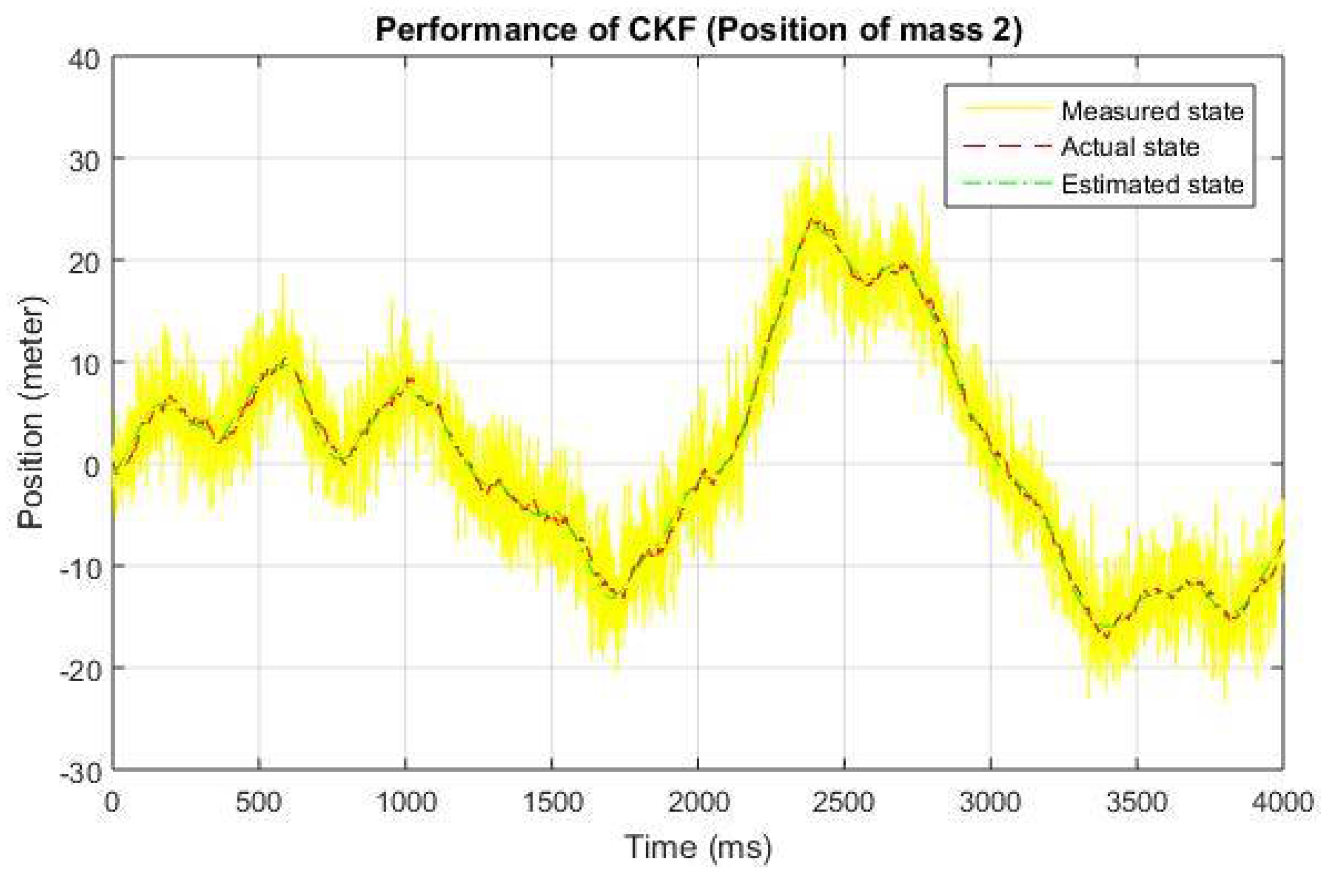
Before introducing the data loss in the estimation process, we present the performance of conventional Kalman filtering. These results have been shown in
Figure 1,
Figure 2 and
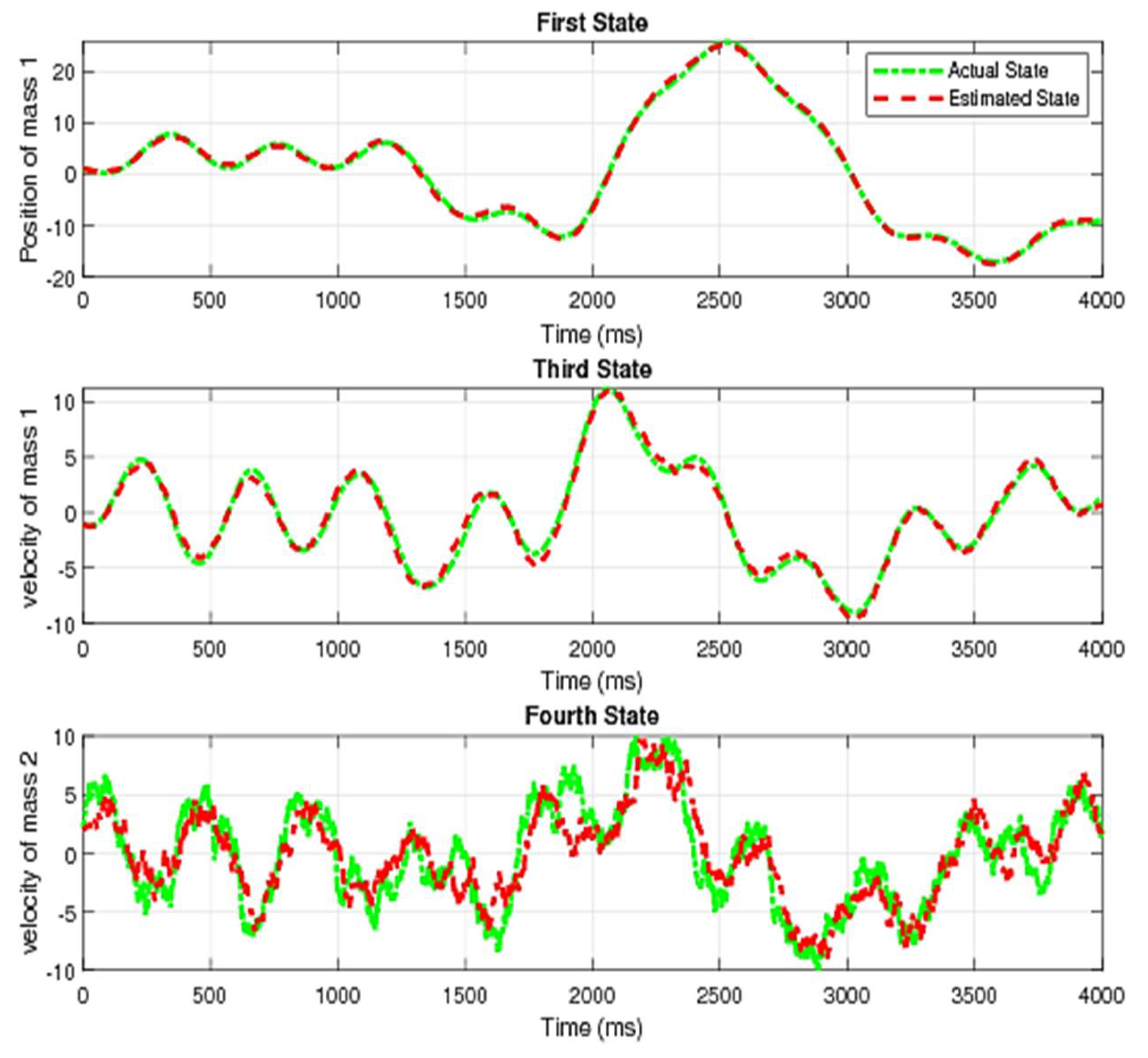
Figure 3, demonstrating three different results for the position of mass m2 of MSD, i.e., measured state shown by the solid line; the actual state represented by the dashed line, and estimated state by convention Kalman filtering given by the dash-dotted line in
Figure 3 consists of three subplots, i.e., first state, third state, and fourth state, each with the actual state shown by the dotted line and the estimated state by convention Kalman filtering represented by the dashed line.
In case of no data loss, the convention Kalman filtering offers satisfactory results obvious from the above figures. The results for some existing remedies and a proposed one and their comparison is made in the next subsection.
5.3. Simulation Results with Data Loss Using Open-Loop Estimation, AR Model, and Proposed ARMAX Model
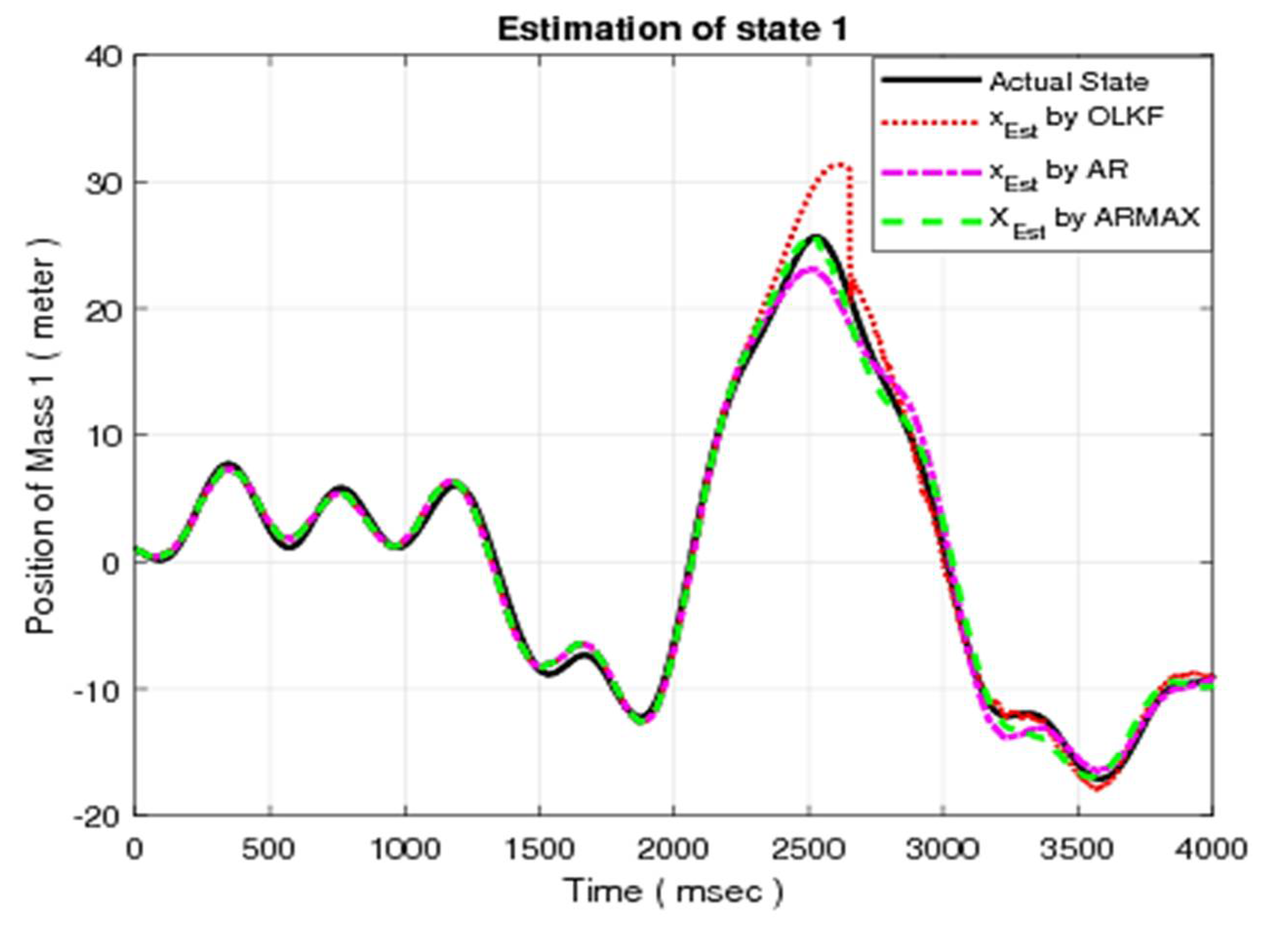
In this section, data loss has been introduced for a period of 415 samples and is inserted from 2235 ms to 2650 ms. The period of data loss can be introduced in any place during the estimation process. Results for existing techniques (OLE, and CLE using AR Model) in comparison with the ARMAX model are presented in the following subsection.
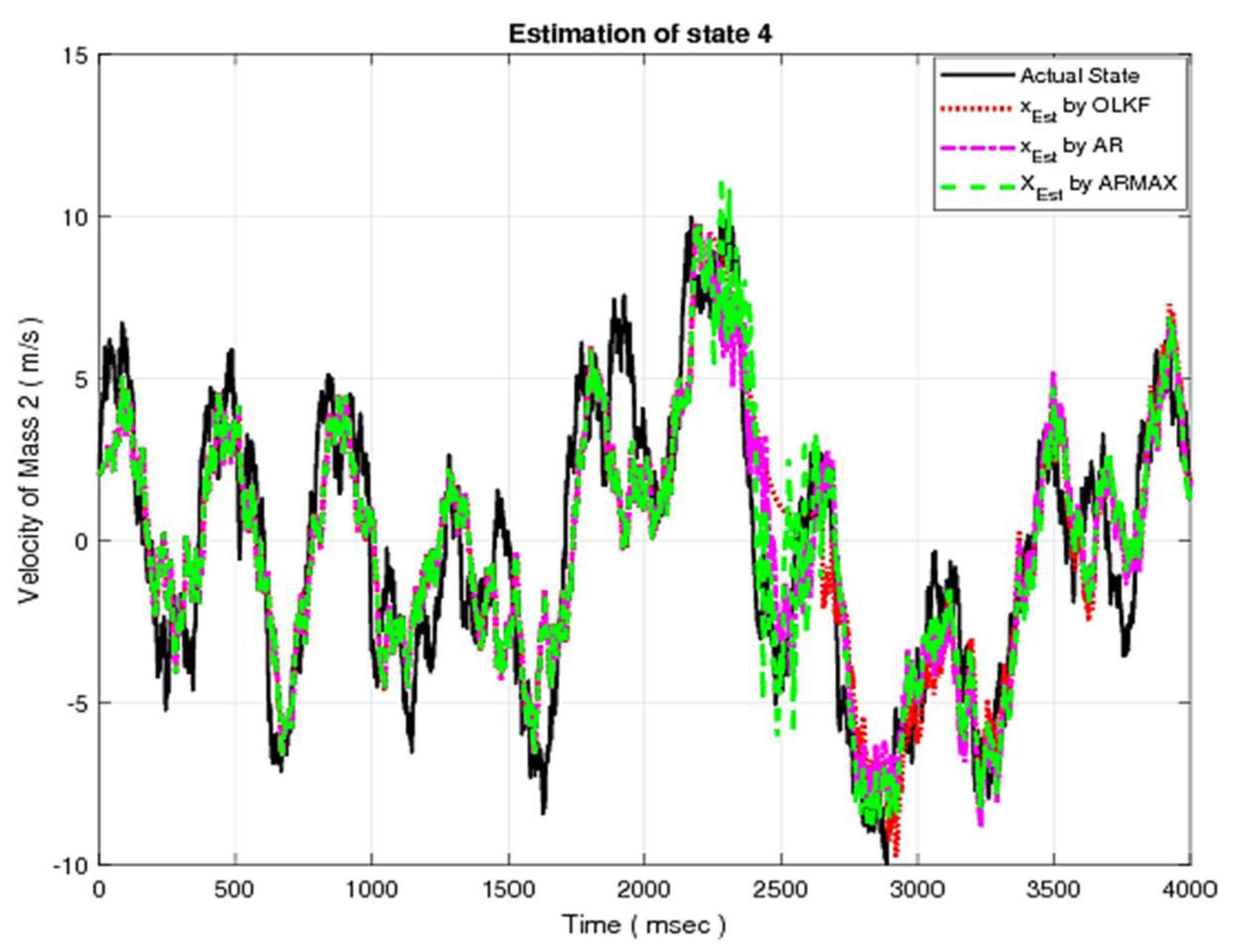
5.3.1. State Estimation
The simulation results for the first state of MSD using the OLE, AR model, and ARMAX model are given in
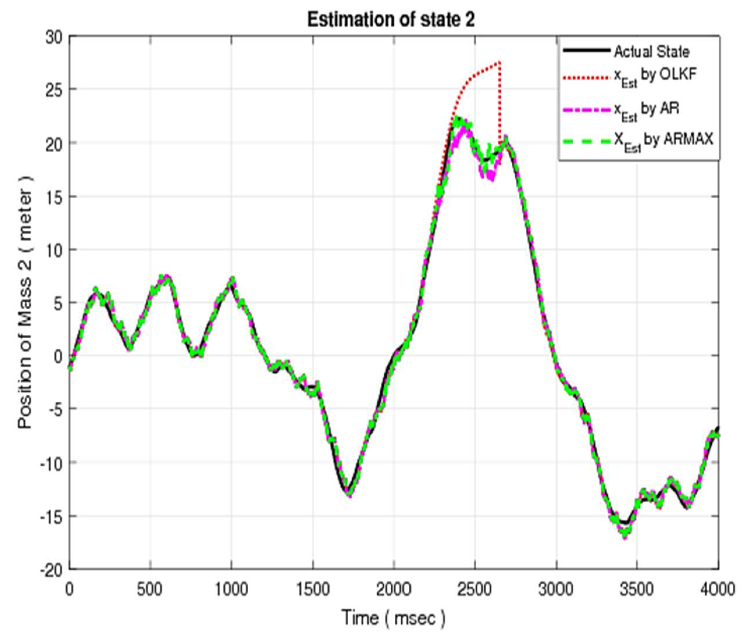
Figure 4. Similarly, the simulation results for other states using OLE, compensated closed-loop (AR model and ARMAX) models are depicted in
Figure 5,
Figure 6 and
Figure 7, respectively.
In each figure, the actual state is shown by the solid line. On the other hand, the estimated states using the OLE, AR model, and ARMAX model are represented by dotted, dashed-dotted, and dashed lines, respectively. It is obvious from the above results that the ARMAX model offers improved compensation as compared with OLE and CLE using the AR model.
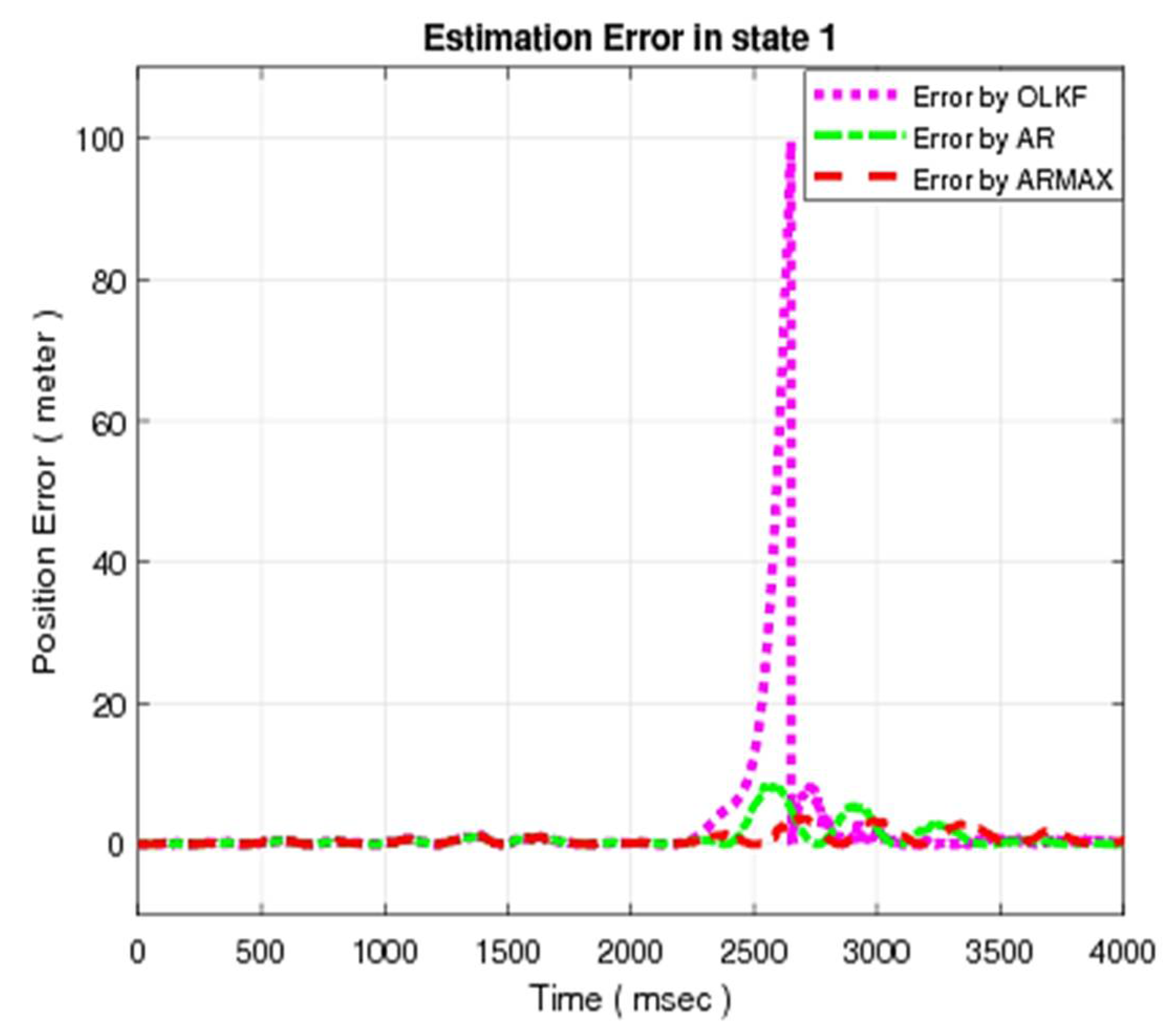
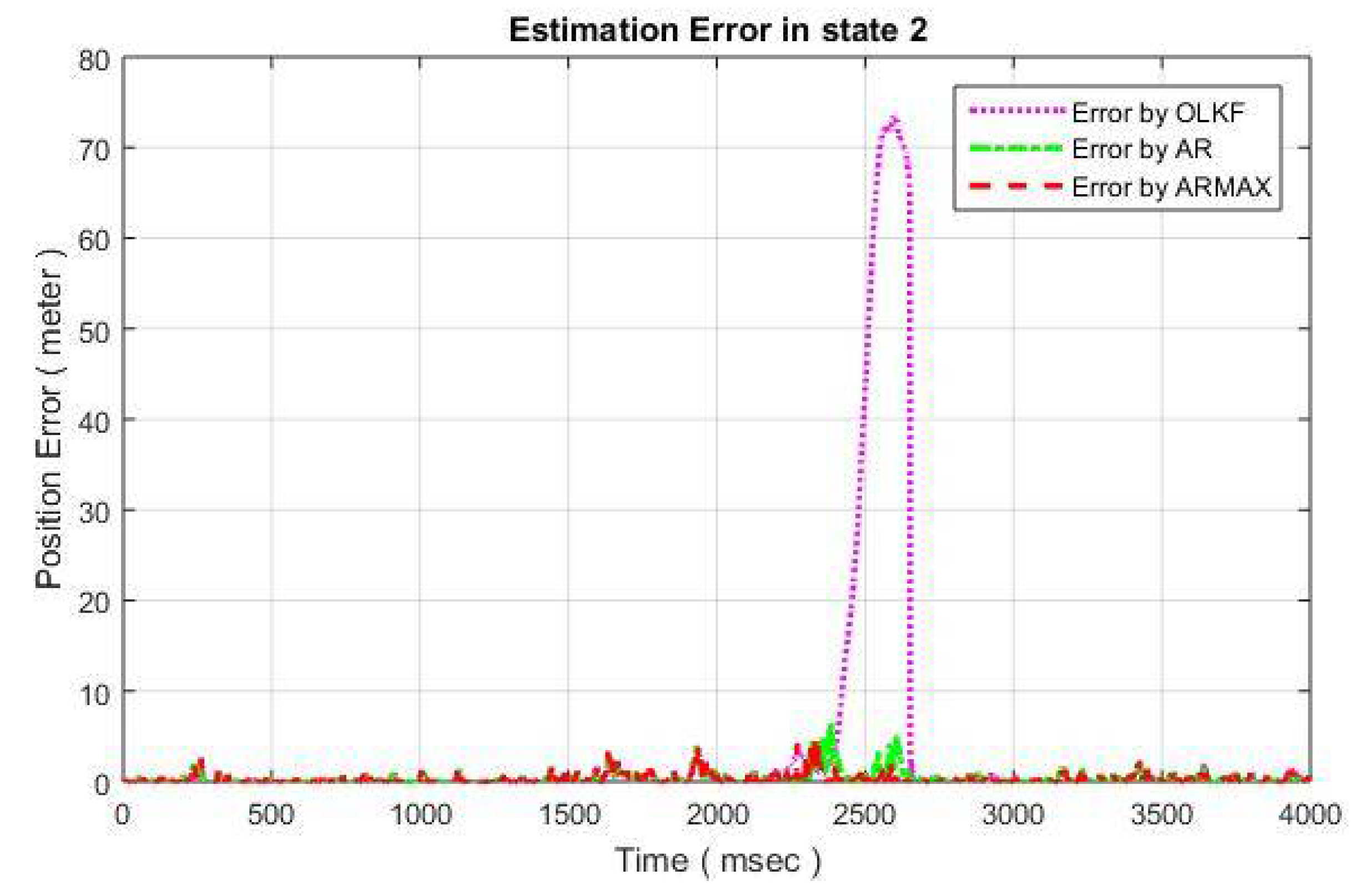
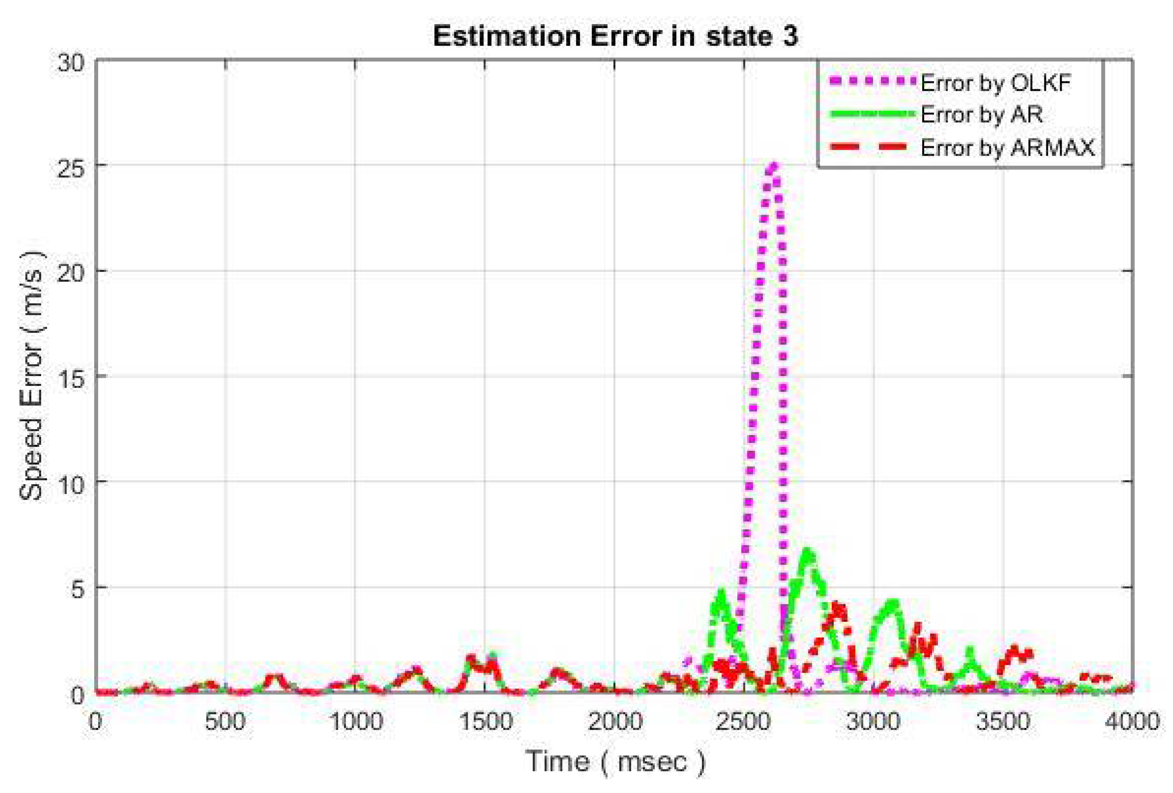
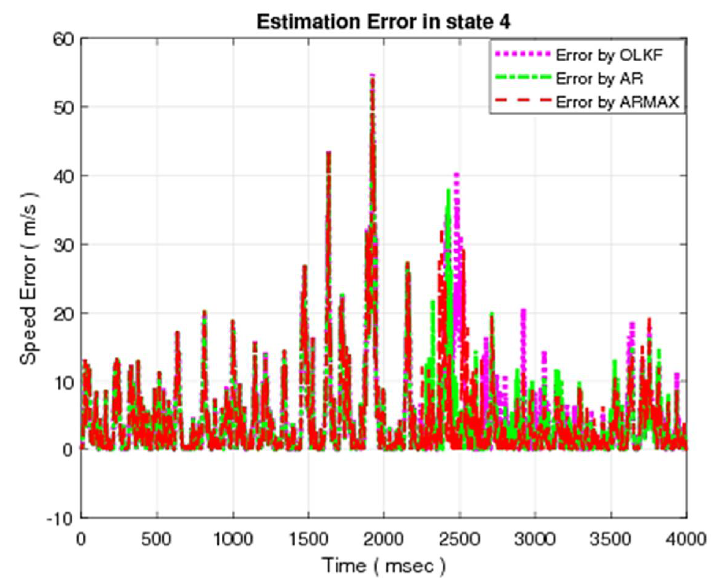
5.3.2. Error Analysis
The error resulting due to compensation for the position of mass
of MSD is depicted in
Figure 8. Similarly, the resulting errors for the other three states are given in
Figure 9,
Figure 10 and
Figure 11, respectively.
Each Figure consists of a dotted line that give the estimation error of the open-loop technique, dashed-dotted which depicts the estimation error resulting due to AR model compensation, and dashed line which presents the error in case of proposed ARMAX model compensation.
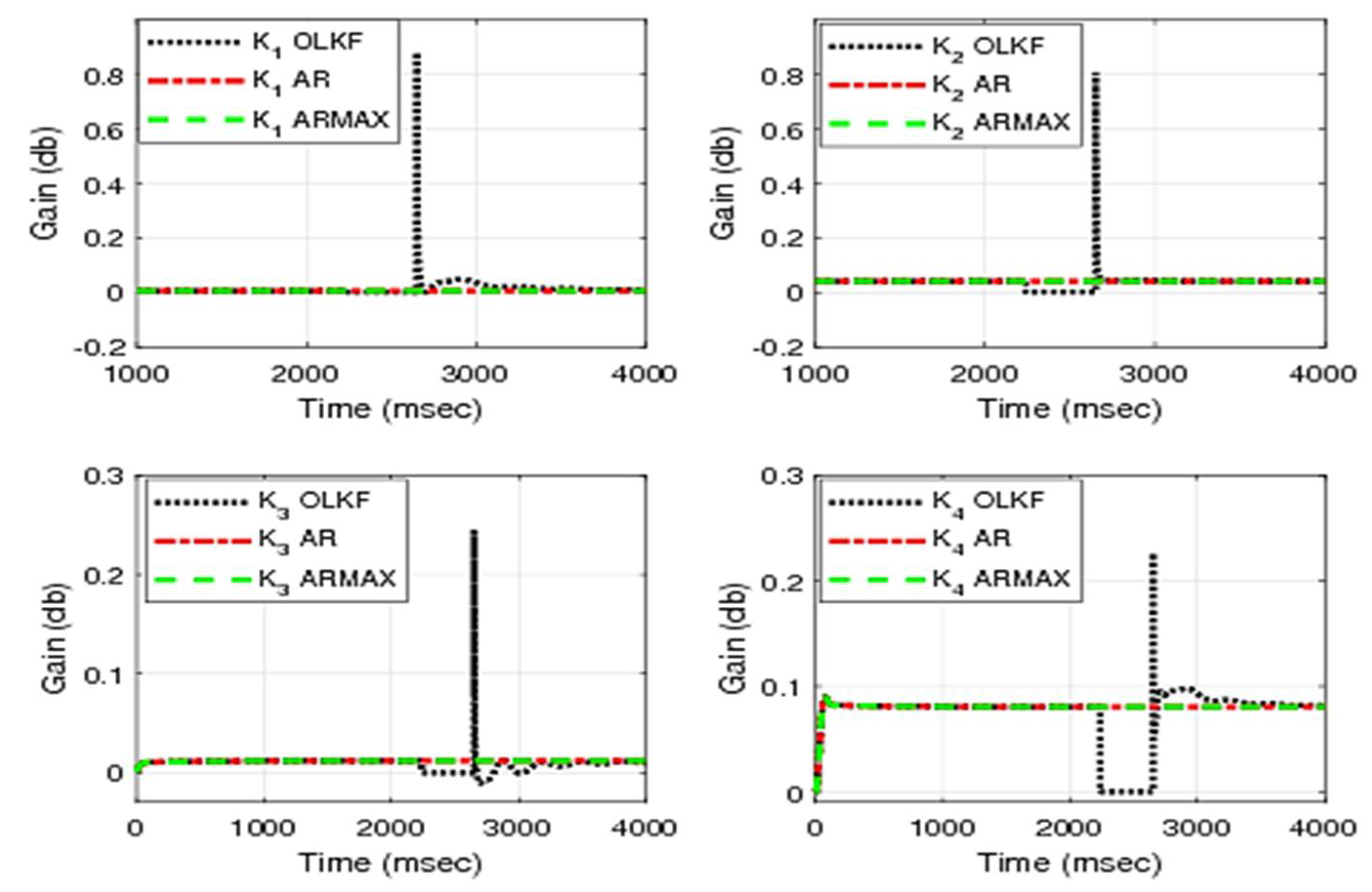
5.3.3. Analysis of Kalman Filter Gain
The variations of Kalman filter gain in case of data loss for the existing techniques (OLE and AR model) and proposed ARMAX are shown in
Figure 12.
During the period of lossy compression, the value of Kalman filter gain is zero for open-loop estimation until the data loss is recovered. In the case of compensated closed-loop techniques using the Kalman filter gain, this is calculated with help of a compensated measurement vector using AR or ARMAX.
6. Conclusions and Future Work
This article presents the estimation technique and proposes an improved compensation when the estimation process is subjected to data loss. In the beginning, the problem of measurement loss is addressed using open-loop estimation with different shortcomings. These disadvantages are overcome by proposing different closed-loop techniques. The earlier closed-loop techniques were based on the autoregressive model with a minimal number of pieces of information. In the proposed model, the amount of information has been increased by taking the measurement, input, and system disturbance for the compensation of missing data samples.
In this work, existing and proposed schemes are based on a linear system. However, most of the time the system under consideration is nonlinear. Therefore, the problem of data loss for a non-linear system is the possible extension of this work.
Author Contributions
Conceptualization, Data curation, Methodology, Resources, Validation, Writing—original draft, Writing—review & editing, S.A.B. and G.A.; Conceptualization, Data curation, Methodology, Resources, Validation, Writing—original draft, Writing—review & editing, Formal analysis, Funding acquisition, Investigation, Project administration, Supervision, and Visualization, G.H. and S.M.; Writing—review & editing, Formal analysis, Funding acquisition, Investigation, Project administration, Supervision, and Visualization, F.R.A. All authors have read and agreed to the published version of the manuscript.
Funding
The APC is funded by Taif University Researchers Supporting Project Number(TURSP-2020/331), Taif University, Taif, Saudi Arabia.
Acknowledgments
The authors would like to acknowledge the support from Taif University Researchers Supporting Project Number (TURSP-2020/331), Taif University, Taif, Saudi Arabia.
Conflicts of Interest
The authors declare no conflict of interest.
References
- Dochain, D. State and parameter estimation in chemical and biochemical processes: A tutorial. J. Process Control 2003, 13, 801–818. [Google Scholar] [CrossRef]
- Khan, N.; Bacha, S.A.; Khan, S.A. Afrasiab Improvement of compensated closed-loop Kalman filtering using autoregressive moving average model. Measurement 2019, 134, 266–279. [Google Scholar] [CrossRef]
- Huang, Y.; Yu, W.; Usman, M.; Wang, S.; García-Ortiz, A. Analysis of Optimal Reconstruction Methods Based on Incomplete Information From Sensor Nodes Using Kalman Filter. IEEE Sens. J. 2018, 18, 6889–6902. [Google Scholar] [CrossRef]
- Khalaf, M.; Hussain, A.J.; Al-Jumeily, D.; Baker, T.; Keight, R.; Lisboa, P.; Fergus, P.; Al Kafri, A.S. A Data Science Methodology Based on Machine Learning Algorithms for Flood Severity Prediction. In Proceedings of the 2018 IEEE Congress on Evolutionary Computation (CEC), Rio de Janeiro, Brazil, 8–13 July 2018; pp. 1–8. [Google Scholar] [CrossRef]
- Khan, N.; Bacha, S.A. Proposing optimal ARMA based model for measurement compensation in the state estimation. In Proceedings of the 2017 International Conference on Frontiers of Information Technology (FIT), Islamabad, Pakistan, 18–20 December 2017; pp. 299–304. [Google Scholar]
- Khan, N. Linear Prediction Approaches to Compensation of Missing Measurements in Kalman Filtering. Ph.D. Thesis, University of Leicester, Leicester, UK, 2011. [Google Scholar]
- Shi, Y.; Fang, H. Kalman filter-based identification for systems with randomly missing measurements in a network environment. Int. J. Control. 2009, 83, 538–551. [Google Scholar] [CrossRef]
- Sinopoli, B.; Schenato, L.; Franceschetti, M.; Poolla, K.; Jordan, M.I.; Sastry, S. Kalman Filtering with Intermittent Observations. IEEE Trans. Autom. Control 2004, 49, 1453–1464. [Google Scholar] [CrossRef]
- Fang, H.; Wu, J.; Shi, Y. Genetic adaptive state estimation with missing input/output data. Proc. Inst. Mech. Eng. Part I J. Syst. Control. Eng. 2010, 224, 611–617. [Google Scholar] [CrossRef]
- Chu, W.C. Speech Coding Algorithms: Foundation and Evolution of Standardized Coders; John Wily and Sons Inc.: Hoboken, NJ, USA, 2003. [Google Scholar]
- Grewal, M.S.; Andrews, A.P. Kalman Filtering: Theory and Practice using MATLAB, 3rd ed.; John Wily and Sons Inc.: Hoboken, NJ, USA, 2008. [Google Scholar]
- Xie, L.; Xie, L. Peak Covariance Stability of a Random Riccati Equation Arising from Kalman Filtering with Observation Losses. J. Syst. Sci. Complex. 2007, 20, 262–272. [Google Scholar] [CrossRef]
- Huang, M.; Dey, S. Stability of Kalman filtering with Markovian packet losses. Automatica 2007, 43, 598–607. [Google Scholar] [CrossRef] [Green Version]
- Khan, N.; Fekri, S.; Gu, D. Improvement on state estimation for discrete-time LTI systems with measurement loss. Measurement 2010, 43, 1609–1622. [Google Scholar] [CrossRef]
- Khan, N.; Khattak, M.I.; Bhatti, T.; Ullah, A.; Shah, S.R. Reduction of computational time for a robust Kalman Filter through Leroux Goguen Algorithm. Tech. J. 2015, 20, 91–97. [Google Scholar]
- Makhoul, J. Linear prediction: A tutorial Review. Proc. IEEE 1975, 63, 561–580. [Google Scholar] [CrossRef]
- Khan, F.; Khan, N.; Khan, L.U.; Khan, M.N.; Pirzada, B. On the optimal frame size of linear prediction techniques. In Proceedings of the 2013 International Conference on Circuits, Power and Computing Technologies (ICCPCT), Nagercoil, India, 20–21 March 2013. [Google Scholar]
- Welch, G.; Bishop, G. An Introduction to Kalman Filter; ACM Inc.: New York, NY, USA, 2001. [Google Scholar]
- Fekri, S.; Athans, M.; Pascoal, A. Robust multiple model adaptive control (RMMAC): A case study. Int. J. Adapt. Control Signal Process. 2007, 21, 1–30. [Google Scholar] [CrossRef]
- Liu, X.; Goldsmith, A. Kalman Filtering with partial observation loss. In Proceedings of the 2004 43rd IEEE Conference on Decision and Control (CDC) (IEEE Cat. No.04CH37601), Nassau, Bahamas, 14–17 December 2004. [Google Scholar]
- Gu, D.W.; Petkov, P.H.; Konstantinov, M.M. Robust Control Design with MATLAB, Advance Textbooks in Control and Signal Processing; Springer: Berlin/Heidelberg, Germany, 2005. [Google Scholar]
- Ugalde-Loo, C.E.; Acha, E.; Licéaga-Castro, E. Multi-machine power system power system state space modeling for small-signal stability assessment. Appl. Math. Model. 2013, 37, 10141–10161. [Google Scholar] [CrossRef]
- Allison, P.D. Missing Data, 1st ed.; SAGE publications: New York, NY, USA, 2001. [Google Scholar]
| Publisher’s Note: MDPI stays neutral with regard to jurisdictional claims in published maps and institutional affiliations. |
© 2021 by the authors. Licensee MDPI, Basel, Switzerland. This article is an open access article distributed under the terms and conditions of the Creative Commons Attribution (CC BY) license (https://creativecommons.org/licenses/by/4.0/).


 ,
, 