Numerical and Experimental Analysis of the Noise Generated in a Ducted Cavity Working in Various Conditions

Abstract

Flow over a cavity or a gap may induce pressure fluctuations that are emitted as sound waves and perceived by a human as noise. This phenomenon may occur in different kinds of industrial machines or in everyday life devices, e.g., cars. For this reason, it is important to predict the flow conditions that intensify or attenuate the noise. This research paper presents the numerical and experimental analysis of the pressure fluctuations in a deep, ducted cavity. The experimental test stand made it possible to investigate the flow over a cavity with air velocity in the range of 30–80 m/s. The pressure fluctuations were measured using miniature microphones located in the duct and the cavity wall and processed with LabView software. The phenomena were also analysed using the computational fluid dynamics (CFD) technique. The several modelling approaches were tested and validated against the experimental data. The highest sound pressure levels were obtained for 40 and 70 m/s. The sound frequency increased with the flow velocity.

1. Introduction

Air flow within cavities is a complex phenomenon that is difficult to investigate using CFD techniques. Applied numerical models need to be carefully validated based on experimental studies. Research on this phenomenon presented in the literature concerns a wide range of flow conditions, including subsonic, transonic, and supersonic flows, where strong wave phenomena occur. Very different geometries and scales of the cavities are considered, depending on their application. The most frequently analysed cases focus on open flows. This type of flow occurs in many elements of machines and devices, such as gas or steam turbines, where the additional influence of rotational effects needs to be considered, e.g., the rim seals between the gas turbine stator and rotor blades.

Such a flow might be a source of instability and noise, which are considered to be unfavorable phenomena. The literature devoted to this subject offers several methods for tackling such problems, e.g., by means of perforated liners that can absorb noise [1].

The current effort is focused on developing appropriate models and tools that will help us better understand and correctly model the presented phenomenon. For this purpose, CFD models that are based on the solutions of the average or filtered Navier–Stokes equations are adopted. The main problem in all types of analysis is the correct modelling of the coupling between the acoustics and the flow field. Hence, a high level of time and spatial discretization are required. The methods based on the solution of the averaged Navier–Stokes equations usually make it possible to determine only tonal noise with a single fundamental frequency. LES [2,3,4] methods and SAS (scale-adaptive simulation) [5,6] or DES (detached eddy simulation) [7,8] methods allow the determination of broadband noise without clearly marked basic frequencies. This type of noise is most often associated with the turbulence generated in high Reynolds flows. An example of the application of the LES method to determine acoustic generation mechanisms that accompany rotating stall and surge in centrifugal compressors at low mass flow rates is given by Sundström et al. [9]. Semlitsch et al. [10] used LES and experimental studies to investigate the relationship between screech tone amplitude and the fluidic injection pressure of the non-ideal expanded supersonic jet. The research presented in this paper is an extension of the work presented in [11,12,13]. The purpose of these works was acoustic and flow analysis using CFD methods, as well as analysis of heat transfer conditions in the case of heated cavities. The authors pointed to the relationship between the strong non-stationary effects generated within the cavity and the heat transfer conditions. These studies were supplemented with partial validation of the applied CFD model, which was presented in [14]. However, these tests were limited to only one basic flow condition. The aim of this paper is to provide a detailed comparison of numerical and experimental research, covering a wide range of flow conditions, including two basic modes of cavity acoustic response along with the transition between these modes. The presented studies concern flow through ducted cavities with a limited span. The obtained experimental results are compared with CFD models that are developed based on the solution of the unsteady RANS equations. The choice of the method is dictated by not only taking into account the correct prediction of acoustic phenomena, but also the efficient modelling of the heat transfer condition within the cavity.

2. Flow Characteristics in A Cavity Area

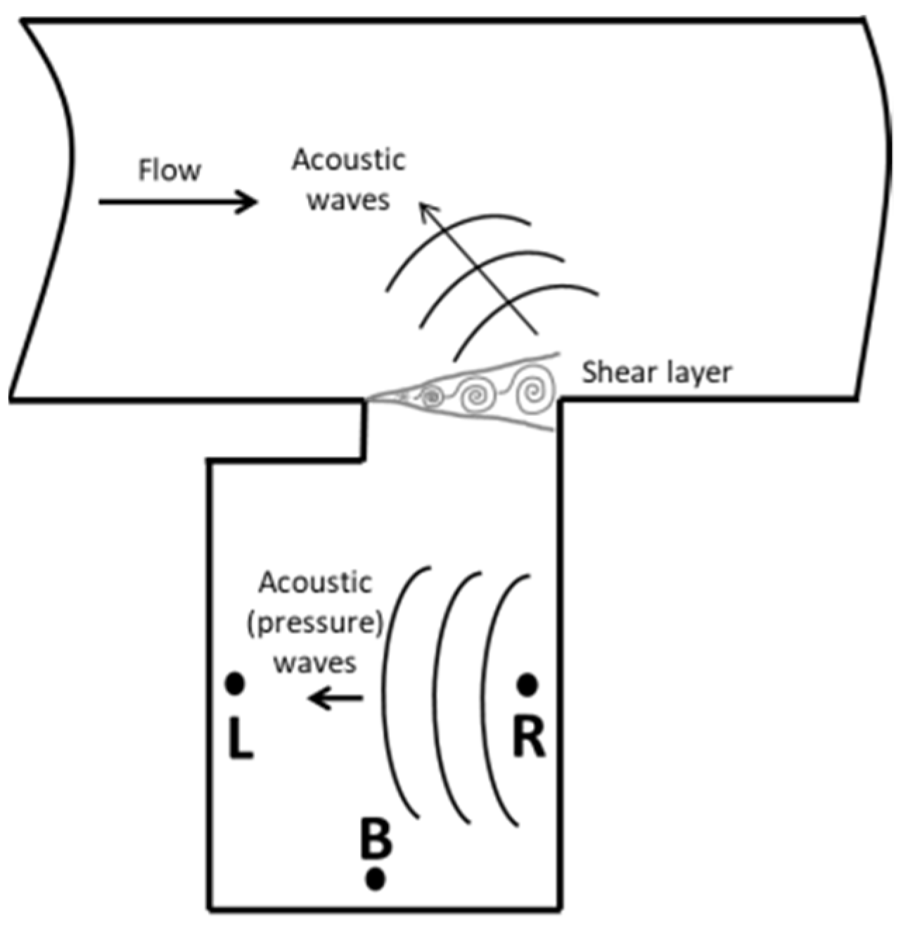
The nature of the flow in an open-type cavity (the type that will be analysed in this work) is determined mainly by the feedback mechanism between the shear layer within the cavity neck and the generated acoustic waves (Figure 1). The acoustic wave is generated by vortices that are formed in the shear layer, which hit the trailing edge of the cavity. They form as a result of Kelvin–Helmholtz instability, which is caused by a significant difference in velocity between the stream flowing over the cavity and the fluid inside. These vortices are formed at the leading edge of the cavity and then are transported along the neck towards the trailing edge, where they collapse and become asource of significant pressure pulsations. This place is treated as an acoustic source, and generated pulsations propagate towards the leading edge at the speed of sound.

The resulting pressure waves, reaching the leading edge of the cavity, affect the shear layer at the point of its detachment, forcing it to generate oscillations with a resonance frequency, depending on the cavity geometry. These oscillations induce the formation of large coherent structures in the shear fluid layer along the cavity neck. These structures are the result of smaller vortices joining under the influence of a moving pressure wave. They are characterized by periodicity and considerable intensity. Hence, the open-type cavities are characterized by a significant level of tonal noise. The mechanism of tonal noise generation in this type of flow was analysed by Rossiter, who proposed a formula to determine the frequency of the pressure pulsations being generated. It is based on the description of the feedback between the generated acoustic wave and the flow of subsequent vortices from the leading edge of the cavity.

Rossiter [15] combined both mechanisms in his model, additionally introducing the value of α, which provides information about the phase shift between the moment of the vortex’s impact on the trailing edge of the cavity and the moment of generation of the acoustic wave. In addition to this, the most common interpretation of the constant α, there are also alternative forms [16,17]. The constant k is usually in the range of 0.5–0.75, while α is in the range of 0–0.25 [18,19]. Both constants are most often chosen empirically. The relationship proposed by Rossiter has the following form:

$$St=\frac{fL}{U_{\infty }}=\frac{m-\alpha }{M_{\infty }+\frac{1}{k}}\hspace{1em}\hspace{1em}\hspace{1em}m=1, 2, 3\dots$$

(1)

where M_∞ is the Mach number of free flow, k = u_c/u_∞ is the ratio of the vortex convective velocity to the main flow velocity u_∞, and λ_fw and λ_fa are the wavelengths that are associated with the frequency of vortex generation and the related acoustic wave, respectively. If this equality is met, it means that there is resonance based on feedback, which significantly amplifies the pressure pulsations that are generated by the cavity.

The second type of resonance that may appear in the analysed cases is the Helmholtz-type resonance [20]. In this case, gas volume in the cavity is subjected to cyclical compression and expansion that results from the compressibility effects. The resonance frequency of the acoustic wave should not depend on the free-stream velocity [21]. This kind of resonance occurs at Mach numbers below 0.2, especially for deep cavities (length/depth < 2) and with a partially closed inlet. The frequency of the acoustic wave produced by the Helmholtz resonator can be described by the relationship:

$$f=\frac{a}{2\pi }\sqrt{\frac{C}{V{b}_{ef}} }.$$

(2)

The frequency of the Helmholtz resonator can also be determined based on the relationship outlined in Equation (3), which is a modification of Equation (2), proposed by Rayleigh [22]:

$$f=\frac{a}{2\pi }\sqrt{\frac{C}{V\left(b+\frac{1}{2}\sqrt{S\pi }\right)}}$$

(3)

In these equations, a denotes the speed of sound, C is the cross-sectional area of the cavity neck, V is the volume of the cavity, b is the height of the neck, and b_ef is the effective height of the cavity neck, which depends on its height b and geometry [21]. In Equation (3), a specific relationship to determine b_ef was assumed. Pressure pulsations arising from the feedback mechanism and related to the Helmholtz-type resonance can occur simultaneously, leading to an increase in pressure pulsation [23].

3. Test Stand and Dedicated Measuring System

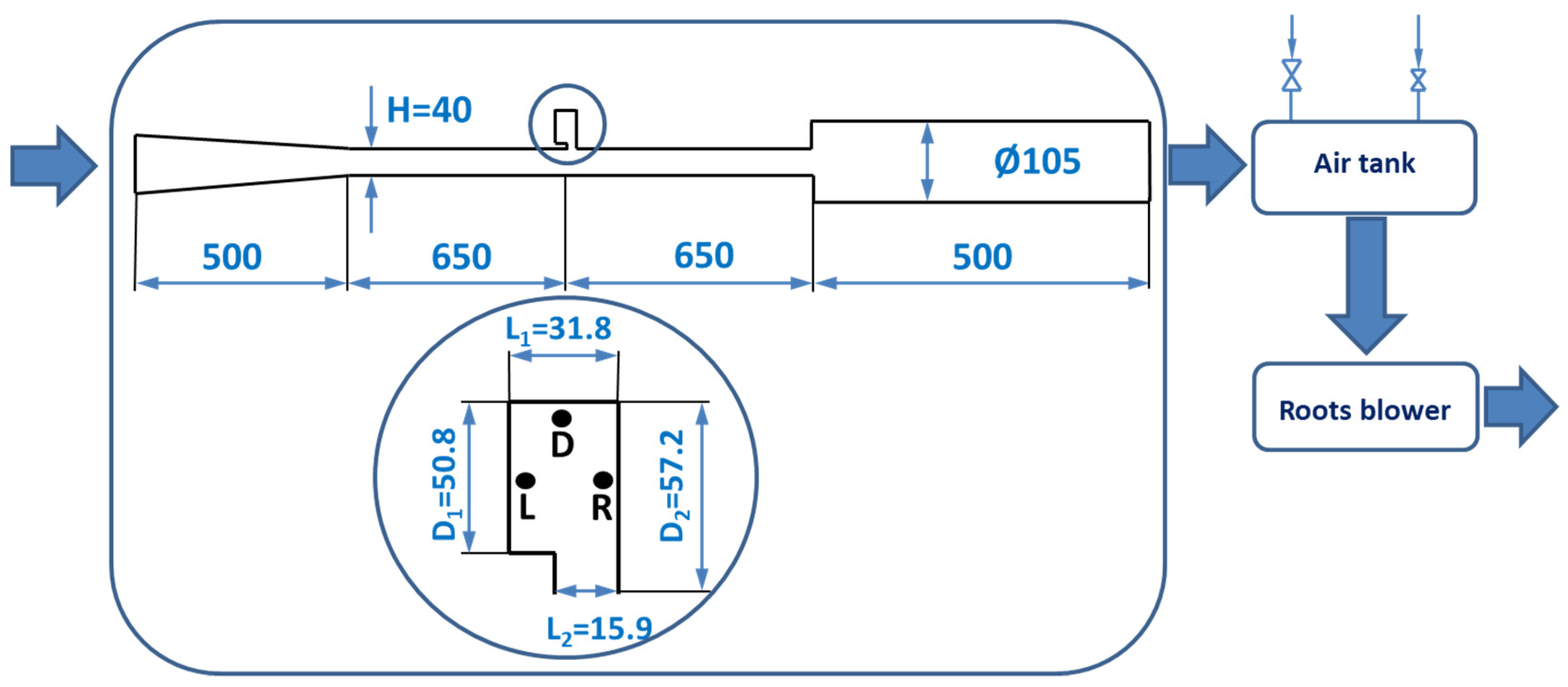
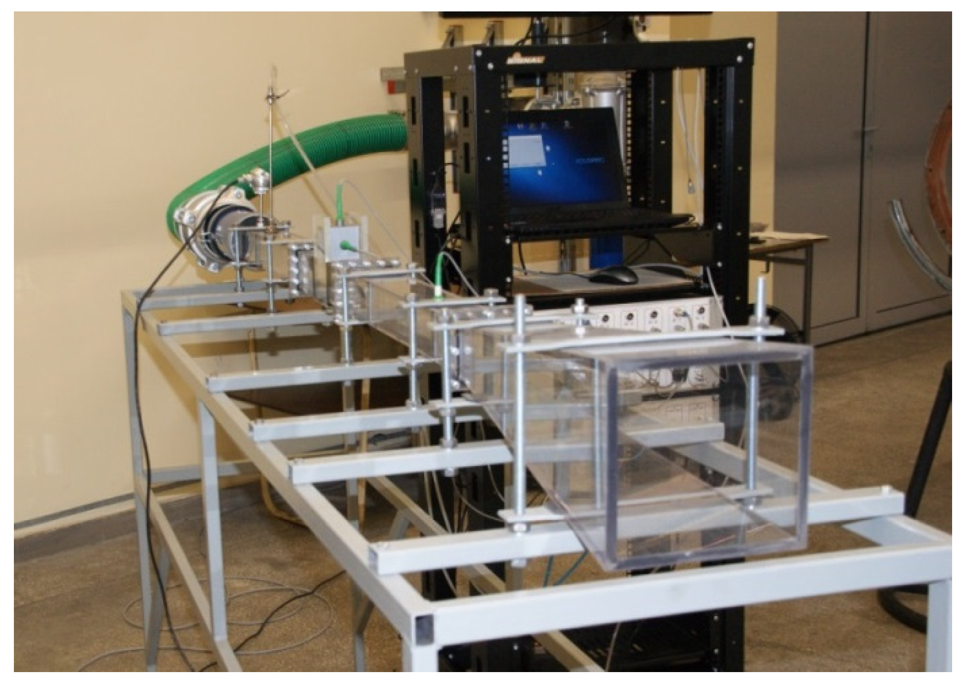
The test stand, with its air preparation system, is presented in Figure 2. The installation is designed to work in negative gauge pressure. The test stand (Figure 3) consists of three main segments. The first is the converging inlet part with an opening angle of 6°. The next part is a rectangular channel with a 50 × 40 mm cross-section. The cavity is located in the middle part of the channel. The last element of the test stand is the transition from a rectangular to circular cross-section and a connection to the air preparation system.

The main element of the air preparation system is the Roots DR124T blower with a maximum flow rate of 12.4 m³/min. It is powered by a 13.2 kW synchronous electric motor, and the maximum negative gauge pressure that it is possible to obtain is 50 kPa. It is directly connected to the 3.2 m³ air tank. The air tank is also equipped with two control valves that control the mass flow rate in the main pipeline. The tank compensates for pressure fluctuations associated with the operation of the Roots blower.

The remaining part of the air system is based on an aluminium pipeline with a diameter of 105 mm.

The test stand measuring system (Figure 4) consists of three main blocks: a fast-changing signals measuring block, a measuring block for slow-changing process parameters, and a data visualization and acquisition block (i.e., a PC with software).

For measurements of the acoustic signals, a set of miniature electret microphones with a diameter of φ = 6 mm was used. The microphones make it possible to record sound pressure levels up to 150 dB (632 Pa). Each of the microphones has a dedicated, adjustable amplifier. A high-power pistonphone was used for the calibration of the acoustic system. The eight microphone amplifiers work with the National Instruments NI USB-6216 measuring module. It is a universal system that includes a 16-channel, 16-bit AC converter with a 400 kS/s sampling rate and which is in communication with a master computer via a serial USB port.

The process signals include reading parameters from two orifices and one thermo-anemometer installed on the pipeline. They enable a precise measurement of the flow rate. In addition, the pressure and temperature of the flowing gas are measured. Direct measurement of velocity on the test stand is possible with the use of Prandtl tubes. The system includes two measuring lines for cooperation with two Pitot probes. All process signals are fed to the ICP DAS universal M-7019 module. This contains a 16-bit, 8-channel converter with a sampling frequency of 8 samples/s. Communication with the master computer is via a serial RS-485 based on the Modbus protocol.

A dedicated program was prepared in the LabView environment to support gathering information from the described measuring modules. The program provides online visualization of fast- and slow-changing signals, FFT analysis, and data recording.

4. Applied CFD Model

The developed CFD model was prepared using Ansys CFX. The software is based on the finite volume method for spatial discretization of Navier–Stokes equations. Time discretization is based on the implicit backward second-order Euler method. The simulations presented in this paper concern the solution of unsteady averaged Navier–Stokes equations (URANS). The air properties were assumed based on the ideal gas law. The viscosity and thermal conductivity of air were dependent on the temperature in accordance with the Sutherland formula [24]. The basic equations solved during the analysis include a continuity Equation (4), a momentum Equation (5), and an energy (6) equation.

$$\frac{\partial \rho }{\partial t}+\frac{\partial }{\partial x_j}\left(\rho U_j\right)=0$$

(4)

$$\frac{\partial \left(\rho U_i\right)}{\partial t}+\frac{\partial }{\partial x_j}\left(\rho U_i{U}_j\right)=-\frac{\partial p}{\partial x_i}+\frac{\partial }{\partial x_j}\left({\tau }_{ij}-\rho \overline{u_i{u}_j}\right)$$

(5)

$$\frac{\partial \left(\rho h_{tot}\right)}{\partial t}-\frac{\partial p}{\partial t}+\frac{\partial }{\partial x_j}\left(\rho U_j{h}_{tot}\right)=\frac{\partial }{\partial x_j}\left(\lambda \frac{\partial T}{\partial x_j}-\rho \overline{u_{j}h}\right)+\frac{\partial }{\partial x_j}\left[U_i\left({\tau }_{ij}-\rho \overline{ u_i{u}_j}\right)\right]$$

(6)

where:

$$\rho \overline{u_{j}h}=\frac{{\mu }_t}{P{r}_t}\frac{\partial h}{\partial x_j}$$

(7)

In Equation (7), Pr_t is a turbulent Prandtl number. Total enthalpy in Equation (6) is defined as:

$$h_{tot}=h+\frac{1}{2}{U}_i{U}_i+k_e$$

(8)

where k_e is turbulence kinetic energy defined according to (9):

$$k_e=\frac{1}{2}\overline{u_i{}^2}$$

(9)

The obtained system of equations is closed using the Boussinesq hypothesis. In this case, the Reynolds stress tensor is expressed based on the average velocity gradient by the introduction of turbulent viscosity μ_t [25] according to Equation (10):

$$-\rho \overline{u_i{u}_j}={\mu }_t\left(\frac{\partial U_i}{\partial x_j}+\frac{\partial U_j}{\partial x_i}\right)-\frac{2}{3}{\delta }_{k{r}_{ ij}}\left(\rho k_e+{\mu }_t\frac{\partial U_k}{\partial x_k}\right)$$

(10)

Taking into account the Boussinesq hypothesis, the averaged momentum equations can be written as:

$$\frac{\partial \left(\rho U_i\right)}{\partial t}+\frac{\partial }{\partial x_j}\left(\rho U_i{U}_j\right)=-\frac{\partial p^{\prime }}{\partial x_i}+\frac{\partial }{\partial x_j}\left[{\mu }_e\left(\frac{\partial U_i}{\partial x_j}+\frac{\partial U_j}{\partial x_i}\right)\right],$$

(11)

where μ_e is a viscosity defined as a sum of molecular viscosity μ and turbulent viscosity μ_t according to (12):

u_e = μ + μ_t

(12)

Additionally, p′ is a modified value of pressure according to (13):

$$p^{\prime }=p+\frac{2}{3}\rho k_e+\frac{2}{3}{\mu }_e\frac{\partial U_k}{\partial x_k}.$$

(13)

The last term in Equation (13) is a velocity divergence and was omitted in the calculations. For the calculations, a two-equation shear stress transport (SST) turbulence model proposed by Menter [26,27] was adopted. This model is a combination of two turbulence models and combines the advantages of the Wilcox k-ω model near the wall and the standard k-ε model in the far field.

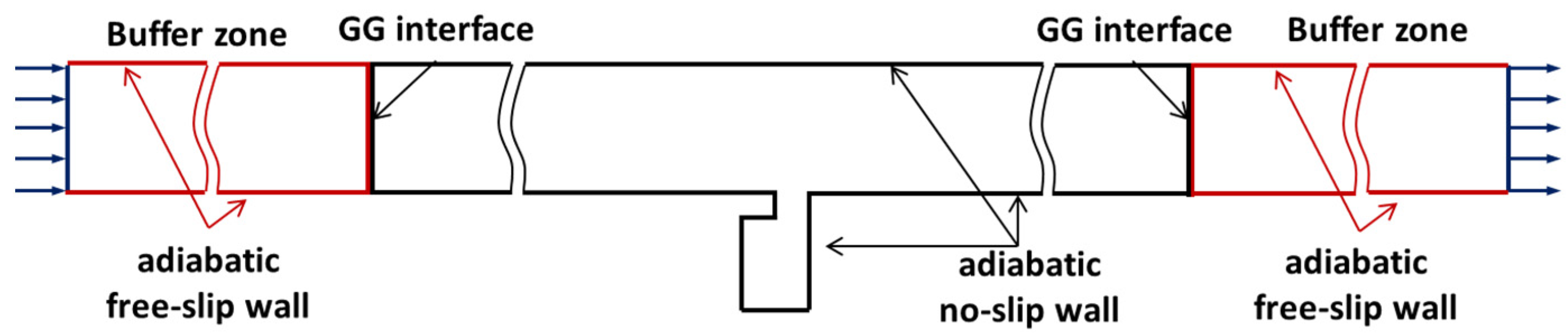
The scheme of the adopted computational domain is shown in Figure 5. The length of the inlet section and its height were assumed according to Figure 2. The computational domain contains two buffer zones where relatively coarse numerical mesh was used. The buffer zones eliminate reflections of the acoustic waves from the assumed boundary conditions.

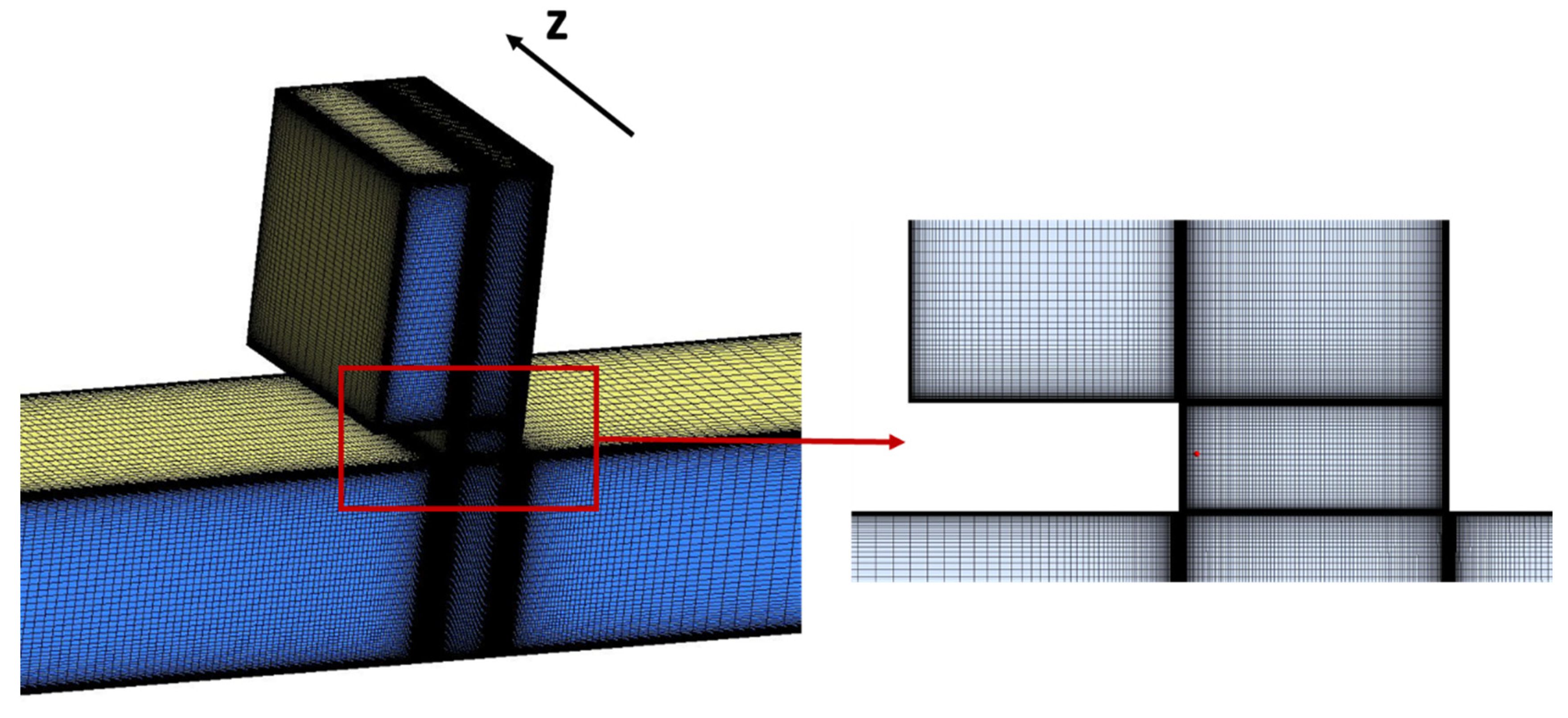
Two main CFD models were investigated, including a basic two-dimensional and a fully three-dimensional computational domain. The numerical mesh was the same in both cases. However, the three-dimensional analysis required proper spatial discretization of the cavity span. For this purpose, 50 elements along the span were used.

This made it possible to take into account the viscosity effects associated with the presence of the lateral walls of the channel and cavity.

The numerical mesh was chosen based on grid-independent studies carried out on a two-dimensional model. Three different sizes of numerical mesh were investigated, including meshes with 140,000, 230,000, and 580,000 nodes. In each case, the generated mesh is considerably denser around the inlet to the cavity. This area is particularly important for the process of correctly modelling the generation and propagation of acoustic waves. For all the walls of both the main channel and the cavity, the dimensionless value y + ≈1 was used. The relative error of the SPL prediction as it pertains to the finest mesh is equal to the 4.4% that occurred in the case of the moderate mesh, and is 40% for the coarse mesh. The frequency of the acoustic waves generated for all three investigated meshes is equal. Based on these results, for further analysis, a moderate mesh with 230,000 nodes was selected.

The three-dimensional mesh was generated by translating the 2D mesh and properly dividing it along the z direction. The applied three-dimensional mesh consists of 5.9 million nodes and is shown in Figure 6.

For most of the cases, obtaining a stable periodicity of pressure fluctuations generated by the cavity required more than 100 ms of simulation. According to the analyses presented in [10], a time step equal to 10⁻⁵ s was adopted for the simulation. It provides 87 time steps for one period of the acoustic wave generated by the cavity in the case where velocity in the main channel is equal to 50 m/s. To ensure correct time discretization for cases where the main flow velocity is above 60 m/s, calculations were carried out for a time step of 2.5 × 10⁻⁶ s. This resulted in 110 steps per one period of an acoustic wave in cases where main flow velocity is equal to 80 m/s. Depending on the adopted time discretization and the investigated main flow velocity, the process of establishing the amplitude of the generated acoustic wave required from 5000 to 24,000 iterations, which translates into a considerable calculation time. The adopted boundary conditions are summarized in

Table 1. Applied boundary conditions.

Inlet	Velocity: 30–80 m/s Static temperature: 15 °C Turbulence intensity: 1%
Outlet	Average static pressure: ~1 bar
Cavity and lateral walls	Adiabatic
Heat transfer	Total energy equation including viscous work terms

.

5. Experimental and Numerical Results

Numerical and experimental studies were conducted for a velocity range of 30–80 m/s. This allowed a detailed validation of the adopted numerical models. The analysed working conditions of the cavity included the typical velocity range at which strong pressure pulsations occur, as well as the transition range where pressure fluctuations vanish. This distinguishes this study from other experimental studies, which are most often limited to a narrow range of velocity. The strong pressure pulsations are associated with various sound generation mechanisms, e.g., the Rossiter feedback mechanism. For each of the analysed variants, FFT analysis was performed for both numerical and experimental tests, enabling the determination of the basic components of noise emitted by the cavity.

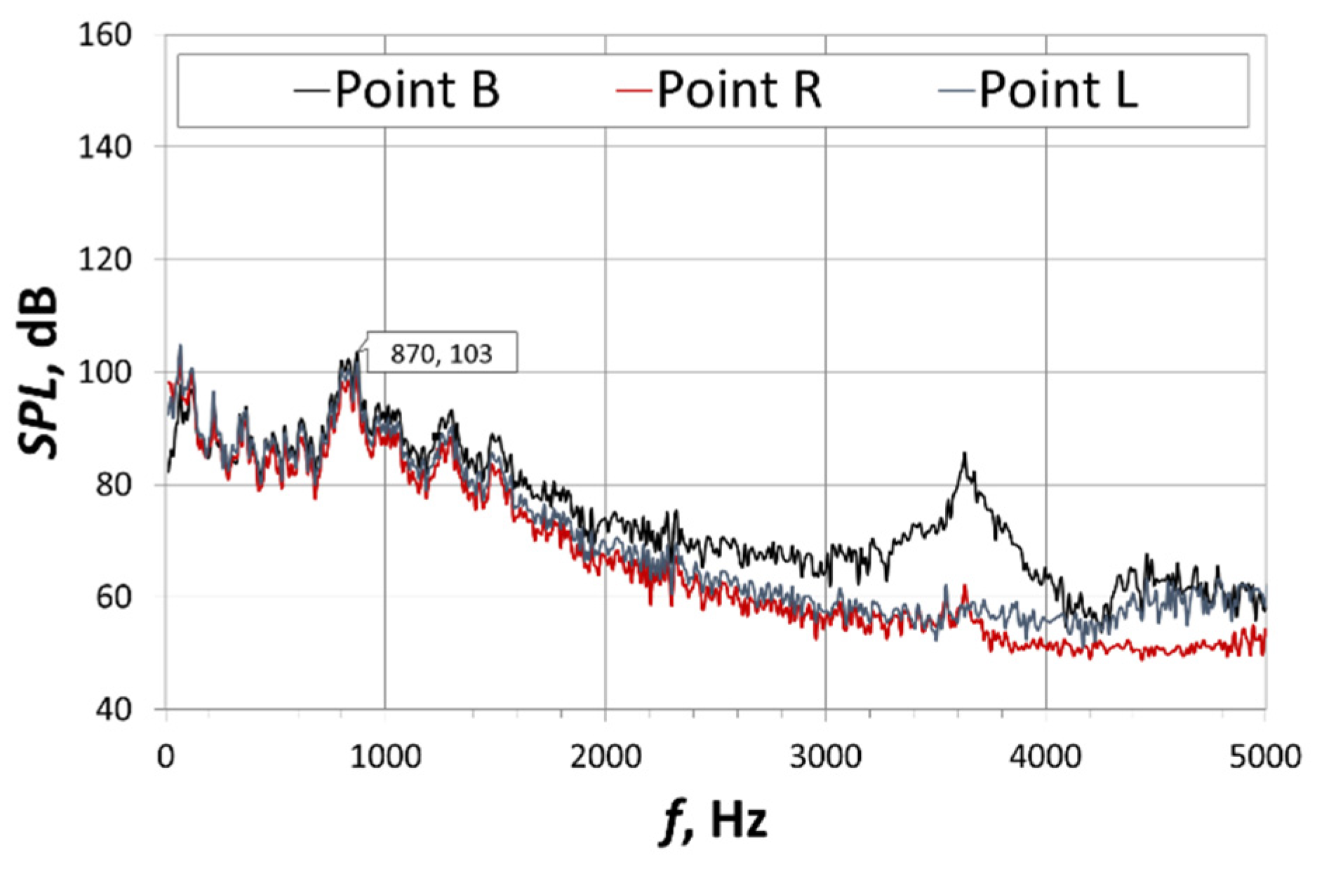
Figure 7 and Figure 8 show the results of the FFT analysis that were obtained in the case of numerical and experimental studies for an average main channel velocity of 30 m/s. The results of the numerical simulations include a two- and three-dimensional model and were obtained for three control points located in the centre of each cavity wall (Figure 1). At this flow rate, as expected, the cavity does not emit strong tonal noise. This is confirmed by the experimental research and the three-dimensional CFD analysis. In both cases, a complex SPL course was obtained without a clearly marked fundamental frequency. The results obtained based on a two-dimensional CFD model vary significantly. In this case, a single fundamental frequency of 781 Hz and subsequent harmonics are visible. However, it is worth emphasizing that the significant differences result from the strongly non-linear nature of the investigated phenomena. This means that pressure pulsations can occur rapidly at a slightly different velocity than predicted by the CFD model.

Strong pressure pulsations that are well visible in both of the CFD models (Figure 9) and in the case of the experimental data (Figure 10) are obtained for the velocity equal to 40 m/s. In this case, the spectrum of the sound pressure level obtained based on numerical simulations is similar to experimental tests. The basic frequency is determined correctly in all cases. The only difference is the lack of a strongly defined second harmonic for the three-dimensional numerical model.

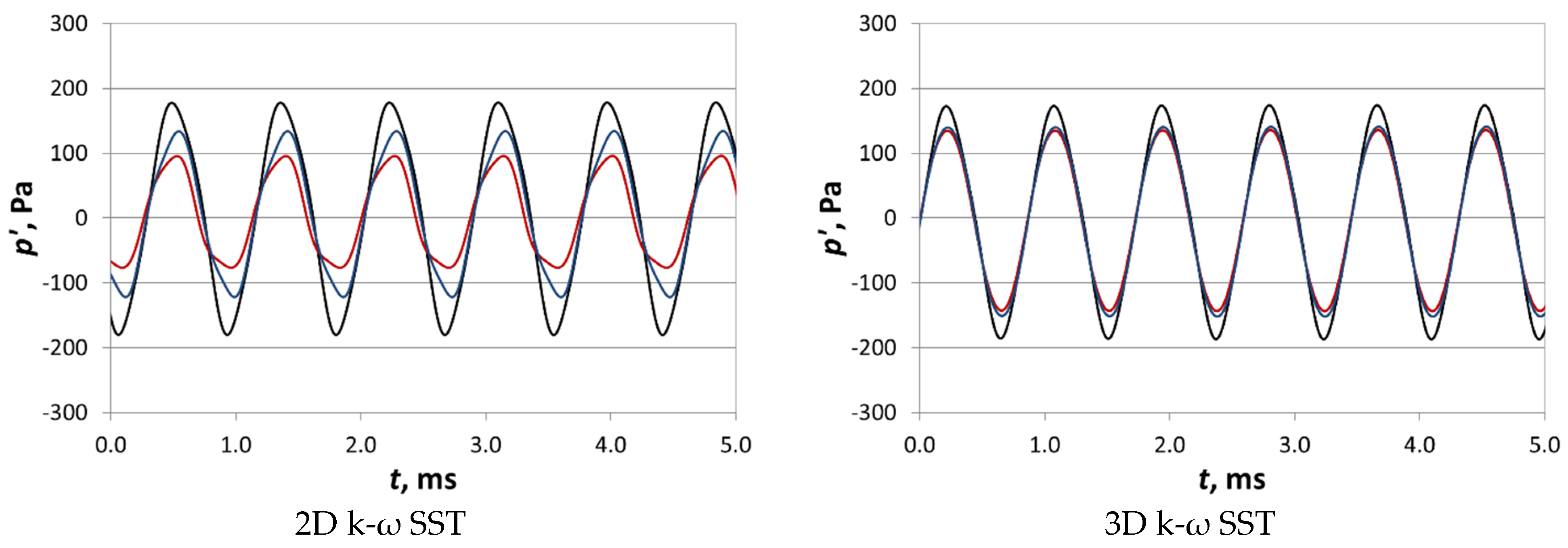
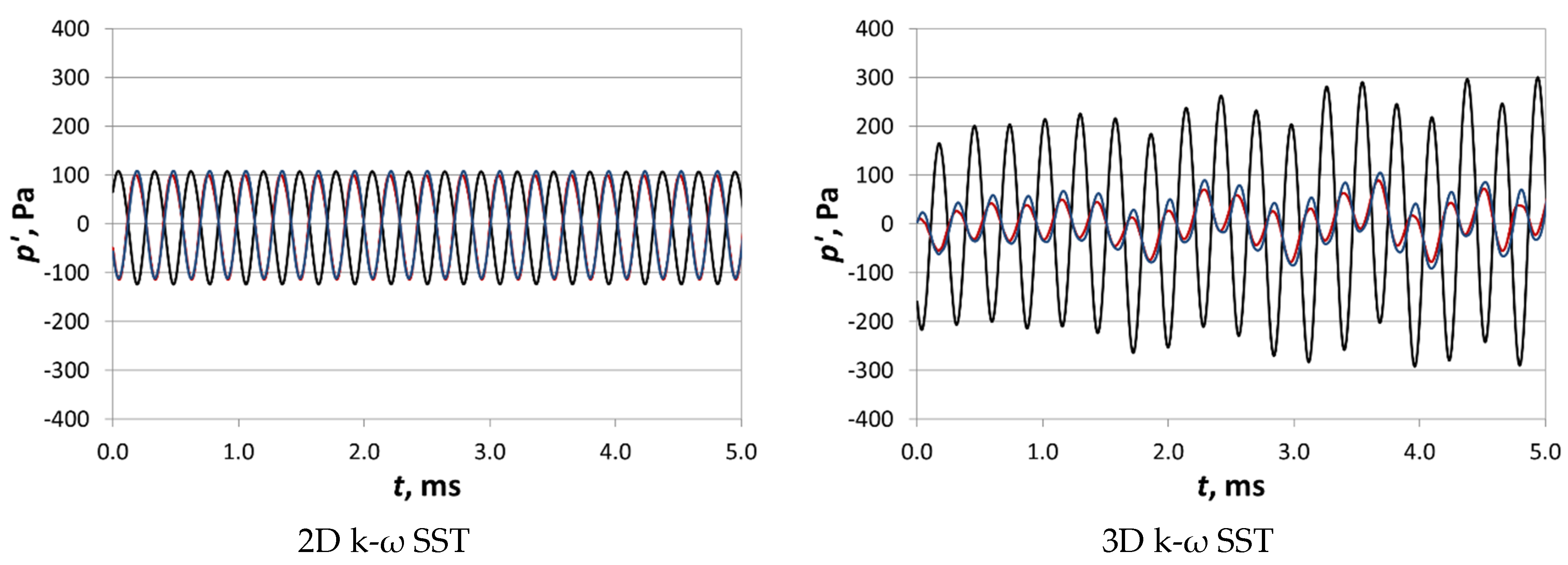
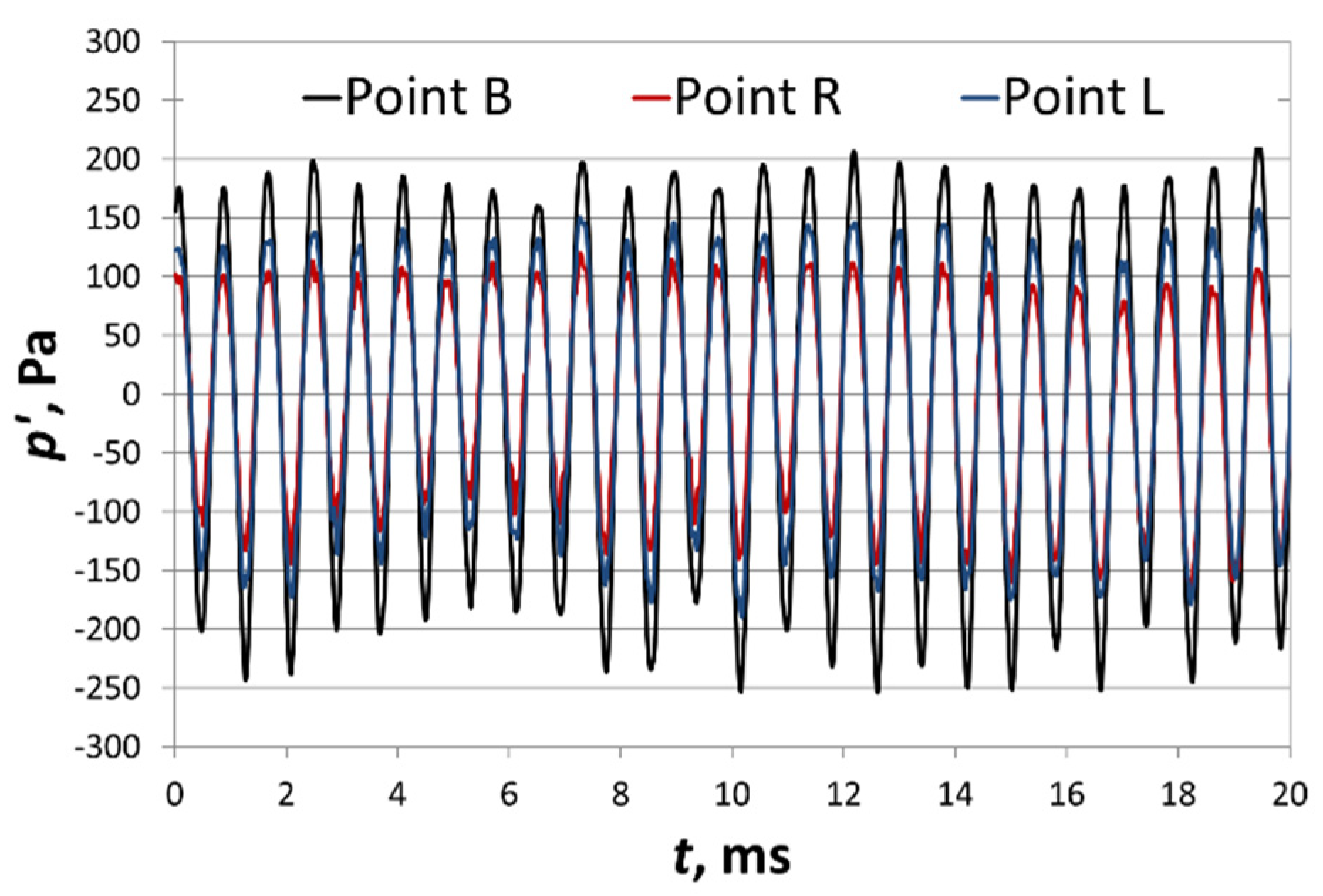
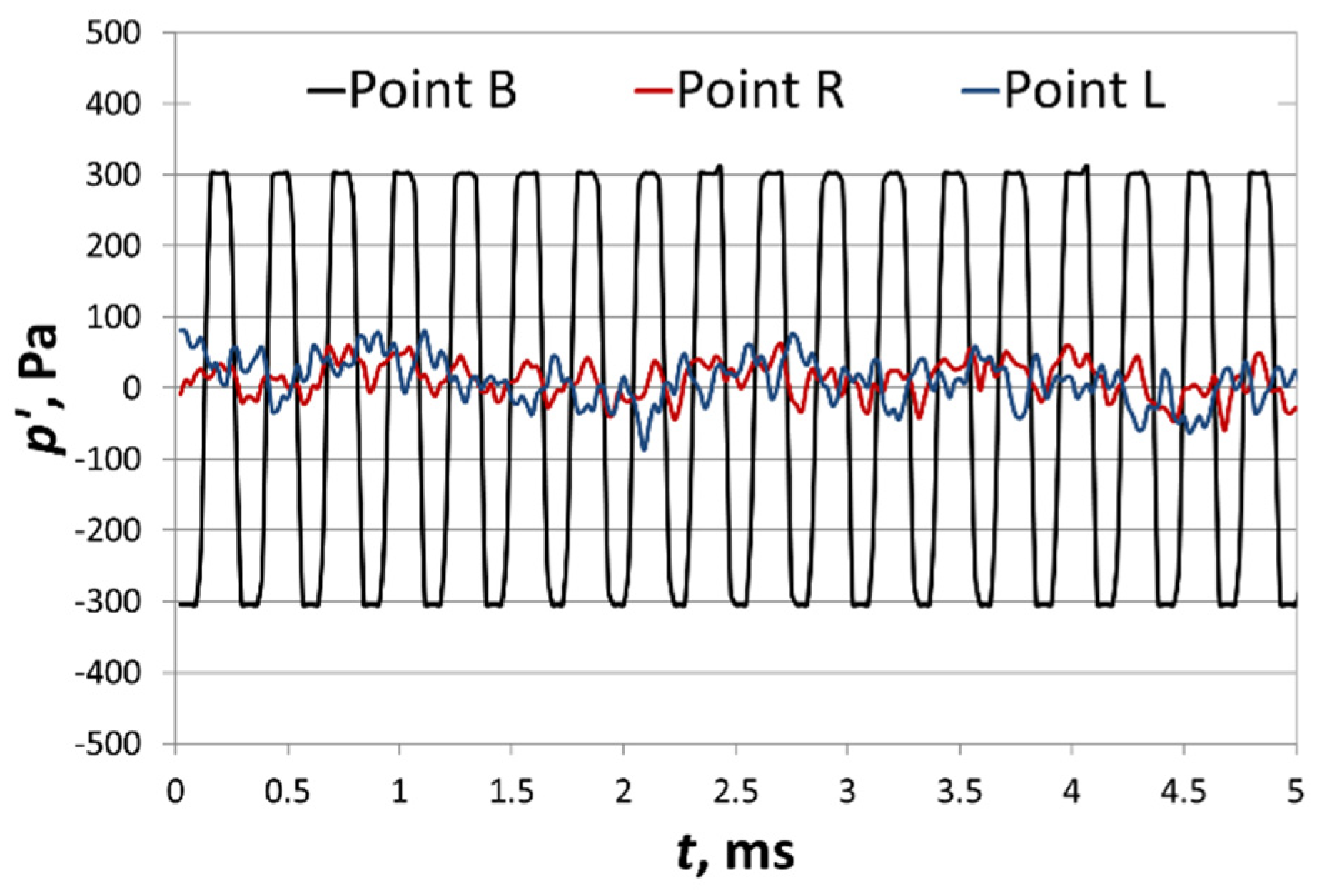
Figure 11 shows a course of the acoustic pressure fluctuations for a flow velocity of 50 m/s, while Figure 12 presents the results obtained based on experimental research. An analysis of the experimental data shows that the acoustic pressure pulsations at 50 m/s are strongly periodic in nature. The waveforms for all three analysed measurement points, including the centre of the left (L), right (R), and bottom cavity wall (B), have sinusoidal waveforms.

The experimental data shows that the amplitude of acoustic fluctuations for points inside the cavity remains invariant. The fluctuation waveforms for all investigated CFD models are alike and characterized by the clearly visible periodicity of the analysed phenomenon. It is also visible in the case of the experimental data. Data collected from the sensors on the cavity walls show that the waveforms of acoustic pressure fluctuations differ in amplitude, but are in phase. This fact proves that this kind of cavity works as a Helmholtz resonator, and pressure pulsations arise in the whole cavity uniformly. Nevertheless, resonance coming from the feedback mechanism described by Rossiter [12] may also appear.

Figure 11. Acoustic pressure fluctuations for velocity in the main channel equal to 50 m/s—CFD.

Figure 11. Acoustic pressure fluctuations for velocity in the main channel equal to 50 m/s—CFD.

Figure 12. Acoustic pressure fluctuations for velocity in the main channel equal to 50 m/s—experimental data.

Figure 12. Acoustic pressure fluctuations for velocity in the main channel equal to 50 m/s—experimental data.

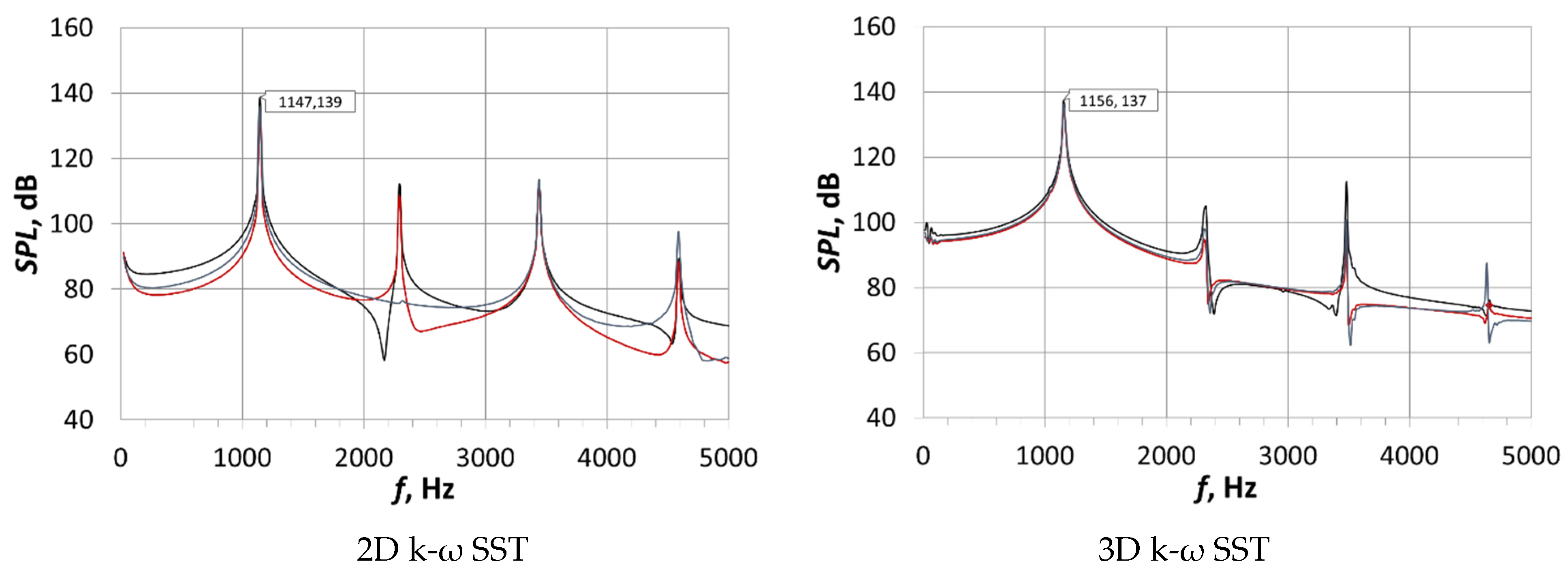
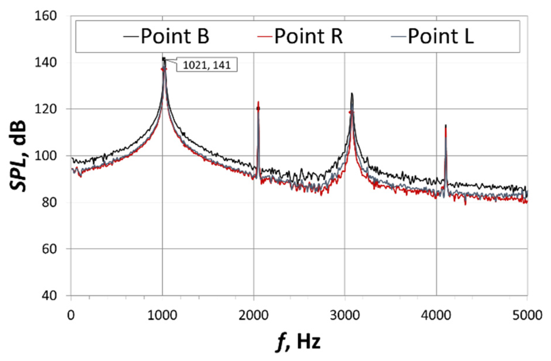
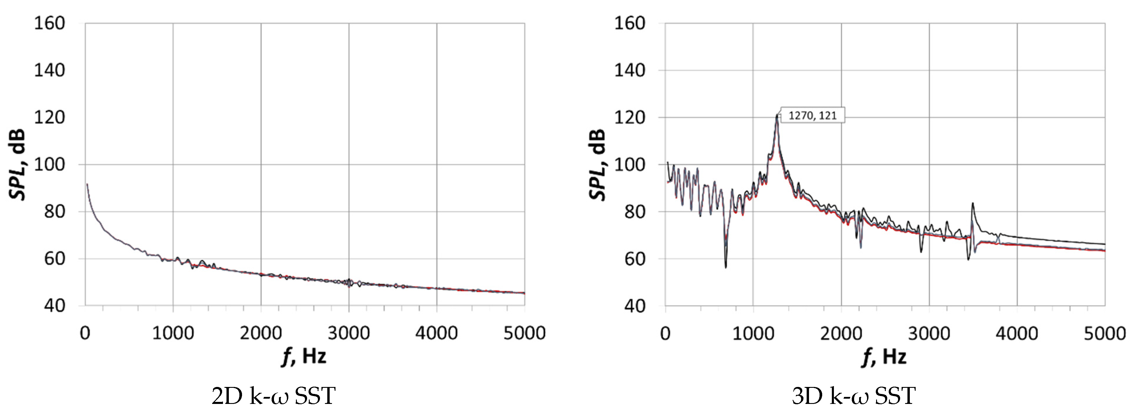
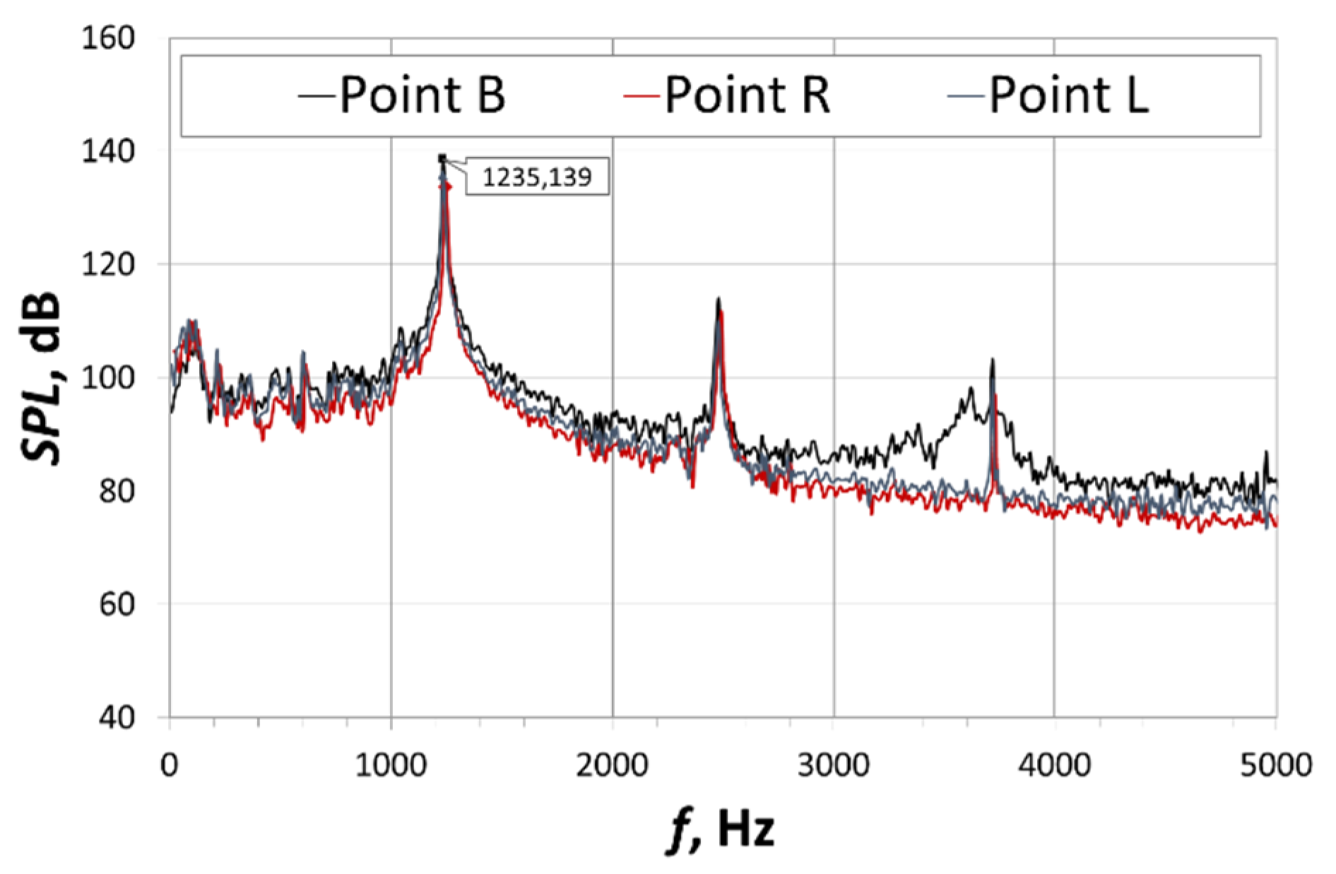
The corresponding FFT analysis is shown in Figure 13 and Figure 14. It is worth highlighting the good agreement between the two-dimensional model, which is significantly simplified, and the more extensive three-dimensional model. The highest and lowest sound pressure levels were achieved at point B (bottom wall) and point R (right wall), respectively.

The relatively low value of the sound pressure at point R is the consequence of its location far below the region where the vortices collide with the wall. Therefore, the higher-pressure pulsations on the right wall of the cavity will occur instead in the vicinity of the main flow channel. The highest discrepancy between the SPL values for the analysed points was obtained in the case of a two-dimensional model.

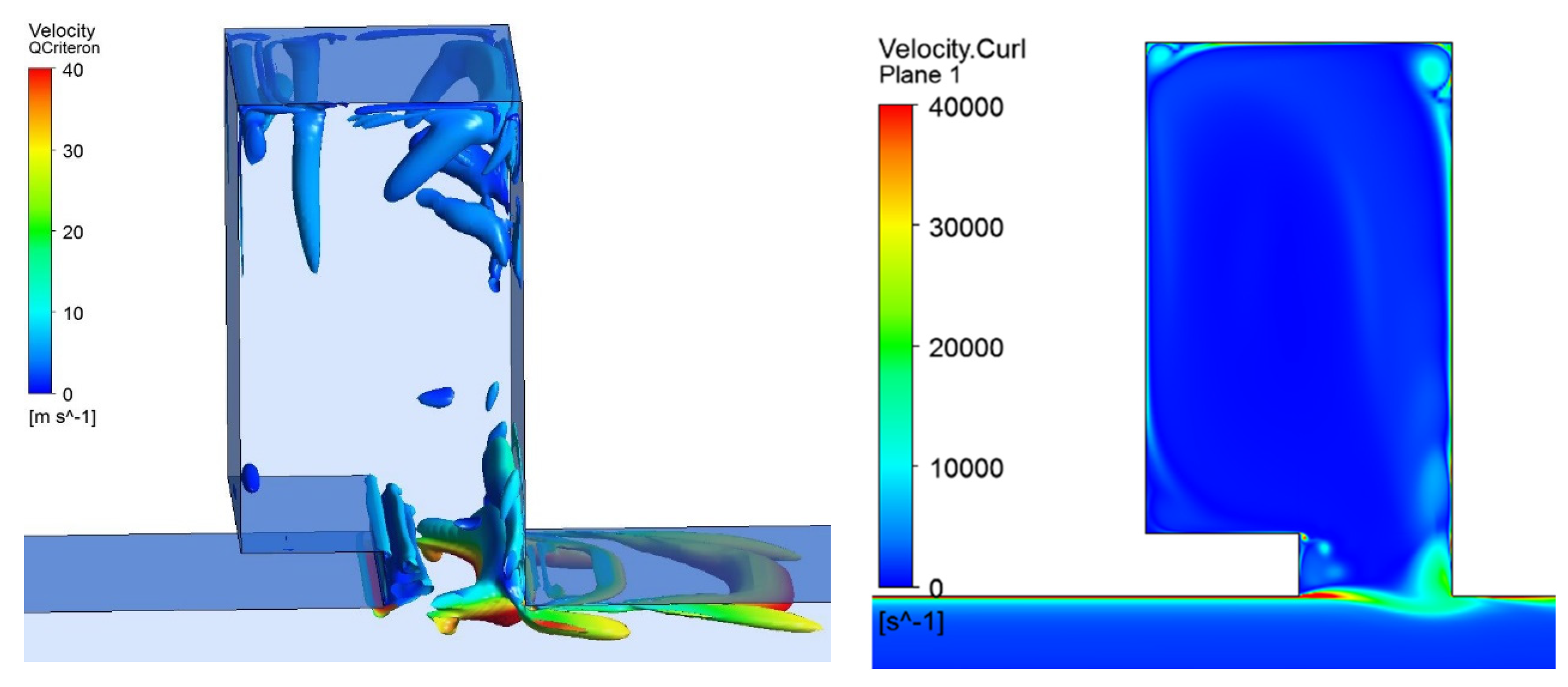
Figure 15 shows the instantaneous Q-criterion and its corresponding vorticity distribution for cavity flow obtained from the three-dimensional CFD analysis. The single, large vortex impingement on the downstream cavity wall is very visible. The strong influence of the lateral walls, which leads to the deflection of the vortex, can be noticed. Additionally, small vortex structures are also formed on the upper part of the upstream cavity neck. Those structures are driven by the circulation inside the cavity and merge with the main vortex path.

It is worth emphasizing that all CFD simulations that include two- and three-dimensional models were carried out assuming a value of the inlet average velocity which corresponded to the flow rate measurement during the experimental studies. This can lead to slightly different flow conditions in the case of the two-dimensional analysis because the influence of the cavity lateral walls is neglected. This can explain some of the differences which occur between those two investigated numerical models. They are especially visible in cases when pressure pulsations arise and are not well established.

Figure 13. Spectral analysis of SPL for velocity in channel equal to 50 m/s—CFD.

Figure 13. Spectral analysis of SPL for velocity in channel equal to 50 m/s—CFD.

Figure 14. Spectral analysis of SPL for velocity in channel equal to 50 m/s—experimental data.

Figure 14. Spectral analysis of SPL for velocity in channel equal to 50 m/s—experimental data.

Figure 15. Instantaneous Q-criterion and vorticity distribution for velocity equal to 50 m/s—CFD.

Figure 15. Instantaneous Q-criterion and vorticity distribution for velocity equal to 50 m/s—CFD.

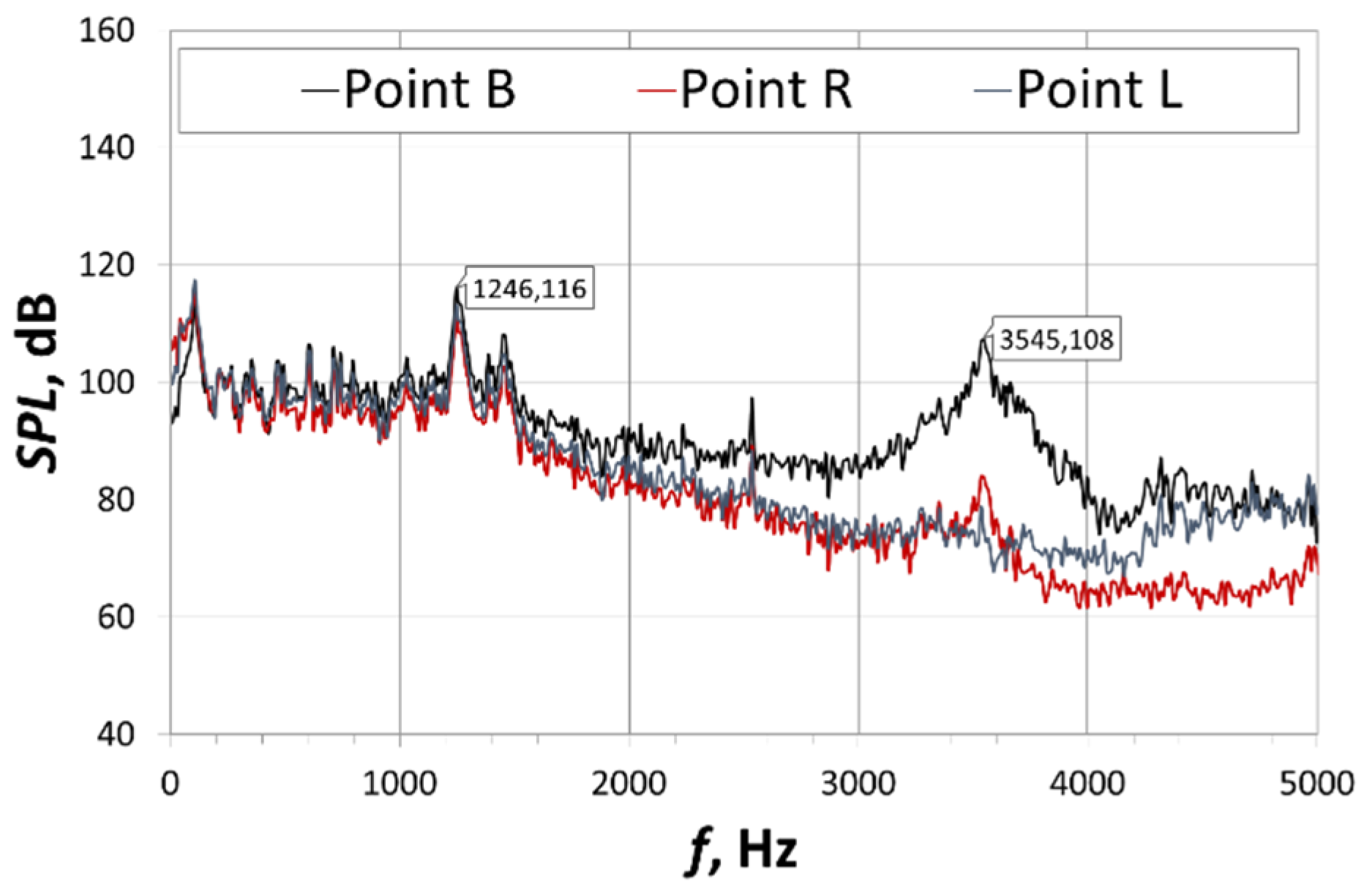
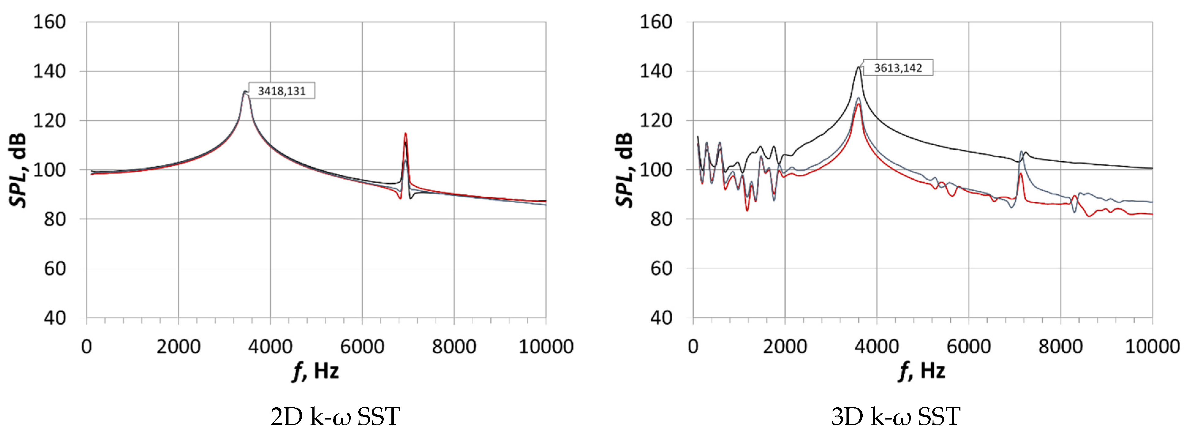
A very important velocity range where the strongly non-linear characteristic of the described phenomenon occurs is 60–70 m/s. Within this range, the pressure fluctuations are extinguished and then re-excite. This phenomenon is accompanied by a significant increase in the frequency of the generated sound wave. The exact point of transition is very difficult to predict. However, when analysing Figure 16 and Figure 17, it can be seen that the results obtained for the three-dimensional numerical model are in fairly good agreement with experimental research. The amplitude of the generated acoustic wave is significantly smaller in comparison to the velocities of 40 m/s and 50 m/s. In addition, a strong second harmonic component with a frequency of about 3500 Hz is visible in the case of the experimental results and the three-dimensional CFD analysis. Full extinction of the acoustic pressure fluctuation was obtained in the case of the two-dimensional analysis. Despite the discrepancies between the CFD models, it should be noted that a small change in velocity equal to 1–2 m/s can lead to the complete extinction of pressure pulsations, as seen in the case of the two-dimensional model.

Figure 18 compares the course of the acoustic pressure fluctuations obtained in the case of two-dimensional and three-dimensional CFD simulations for a flow velocity of 70 m/s and Figure 19 shows the corresponding experimental data. An analysis of the pressure fluctuations course for the three measuring points (Figure 1) shows that a sinusoidal wave is obtained, similar to the velocity of 50 m/s. There are, however, several significant differences between the nature of the pressure fluctuation at 50 m/s and the considered higher flow rates. The results of the CFD analysis show that at 70 m/s and 80 m/s, the acoustic pressure fluctuations at the bottom of the cavity (point B) are in the opposite phase to the points located on the sidewalls of the cavity (points L and R). Therefore, in this case, there is a classic feedback mechanism, which was described by Rossiter. The second important difference is the significant variations in the waveform of sound pressure fluctuations obtained based on two- and three-dimensional analysis.

In the case of the two-dimensional analysis for a velocity of 70 m/s, the obtained pressure fluctuations achieve the same amplitude for all three measuring points, although there is a phase shift between point B and points L and R. This amplitude is about 100 Pa. The three-dimensional numerical analysis shows significant differences in the course of the acoustic pressure fluctuations, especially on the sidewalls of the cavity. The amplitude of the pressure fluctuations is much smaller, although the fluctuation course itself is also sinusoidal.

Figure 18. Acoustic pressure fluctuations for the main flow channel velocity equal to 70 m/s—CFD.

Figure 18. Acoustic pressure fluctuations for the main flow channel velocity equal to 70 m/s—CFD.

Figure 19. Acoustic pressure fluctuations for velocity in the channel equal to 70 m/s—experimental data.

Figure 19. Acoustic pressure fluctuations for velocity in the channel equal to 70 m/s—experimental data.

For point B the pulsation amplitude reaches about 200 Pa, and for points L and R it is about 80–100 Pa. Similar results were obtained based on the experimental research. It is also worth emphasizing that for a velocity of 70 m/s, the obtained pressure fluctuation values for a three-dimensional model coincide with the experimental research, and the two-dimensional analysis gives underestimated results.

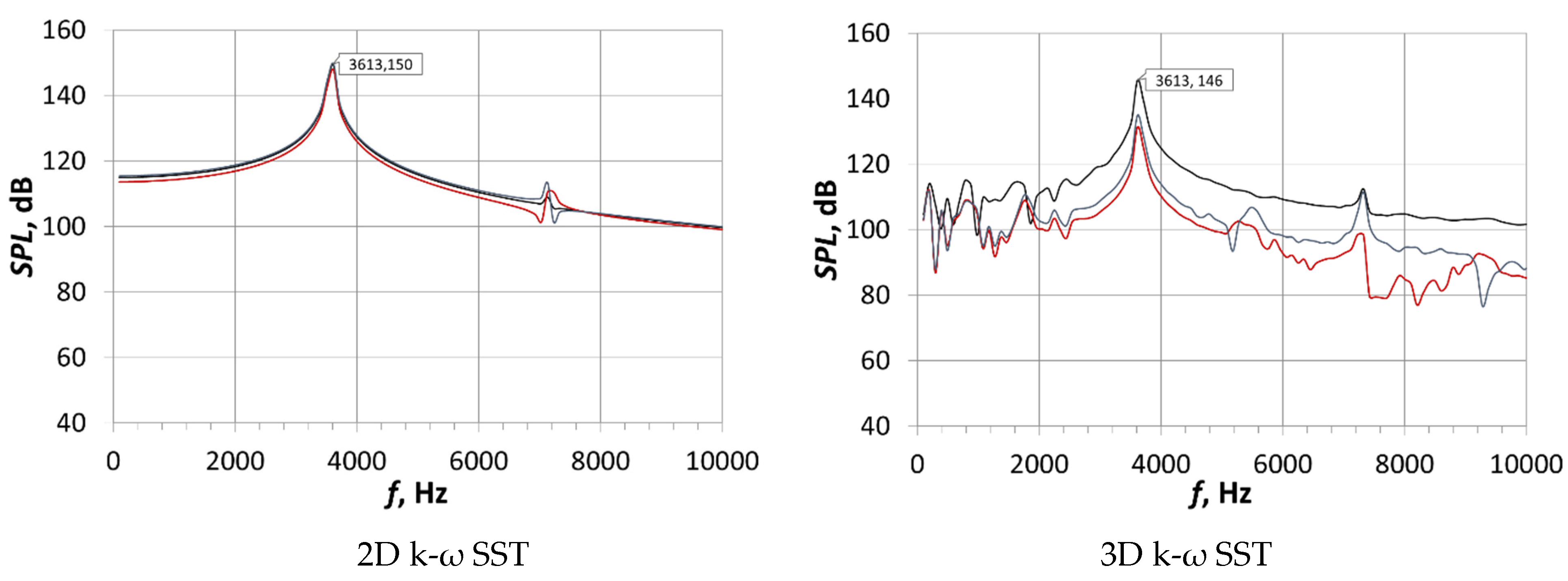
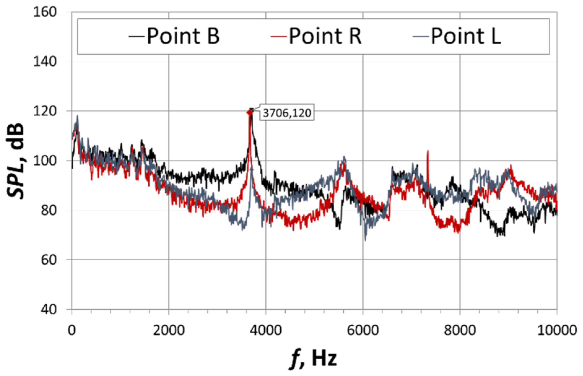
Figure 20 and Figure 21 show the corresponding sound pressure level spectrum for a main channel velocity of 70 m/s. The step change in the frequency of the generated acoustic wave, which reaches the value of 3663 Hz, is visible. For a velocity of 50 m/s, it was 1235 Hz. The beginning of the change in the frequency of the generated acoustic wave was already visible at a velocity of 60 m/s (Figure 17).

In this case, two well-marked harmonics were visible, but the component with a frequency of 1257 Hz and a sound pressure level of 110.6 dB was still dominant.

Very good agreement was obtained in terms of the frequency and sound pressure levels between the experimental and numerical studies, including the applied two-dimensional CFD model. Figure 22 shows the spectral analysis of the sound pressure level for a flow velocity of 80 m/s, and Figure 23 presents the corresponding results of the experimental tests.

For all of the analysed CFD models, the value of the sound pressure level was close to 150 dB, while during the experimental tests the obtained value reached only 120 dB. The jump in frequency is associated with the appearance of a second vortex within the cavity neck. This phenomenon was discussed more extensively in [9]. The frequency and sound pressure levels of the first harmonic for the flow velocity range of 30–80 m/s in the main channel are presented in

Table 2. Parameters of the generated acoustic wave for the velocity range 30–80 m/s.

u, m/s	Experiment	k-ω SST 2D	k-ω SST 3D	Experiment	k-ω SST 2D	k-ω SST 3D
	f, Hz	f, Hz	f, Hz	SPL, dB	SPL, dB	SPL, dB
30	-	781	-	-	125.9	-
40	1021	977	1025	141.4	135.4	142.0
50	1235	1147	1156	138.5	138.8	137.4
60	1246	-	1270	116.0	-	121.0
70	3663	3418	3613	143.7	131.2	141.5
80	37063	3613	3613	119.4	149.7	145.7

.

An analysis of the obtained data shows that both the two- and three-dimensional models give similar results that are consistent with the experimental research, except for a velocity of 80 m/s. For this velocity, CFD models greatly overestimate the sound pressure level, and the difference to the experimental studies is 26.3–30.3 dB, which is 22–25%. Higher discrepancies compared to experimental studies were obtained for the analysed two-dimensional model, which additionally in some velocity ranges imprecisely determines the point of excitation and extinction of the acoustic pressure fluctuations. The best agreement was obtained for 40 m/s and 50 m/s. In this case, for a two-dimensional model, the difference with the experimental research in terms of frequency determination is 4–7.0%, while for the sound pressure level it is up to 4%. For the applied three-dimensional model, it is below 1% both for the frequency and sound pressure levels.

6. Summary

The experimental and CFD research presented in this paper concerned a velocity range of 30–80 m/s. The applied numerical models included simplified two-dimensional and advanced three-dimensional models. They were based on the solution of averaged Navier–Stokes equations, and the two-equation model of turbulence k-ω SST was used to model the Reynolds stress tensor.

The obtained numerical results are characterized by good agreement with experimental data, taking into account the frequency and amplitude of the generated acoustic wave. For the velocity range of 30–70 m/s, the maximum difference in comparison to the experimental data was 6.7% for the predicted frequency, and 8.7% for the sound pressure level. In addition, the three-dimensional model correctly captured the transition from the first to the second mode of pressure pulsations generated by the cavity. This transition is also visible in the case of the adopted two-dimensional model, but the moment of the transition is slightly shifted, which is reflected in the discrepancy in the results obtained for a velocity of 60 m/s.

The greatest difference between the experimental and numerical studies was obtained for a velocity of 80 m/s. In this case, all numerical models correctly predicted the sound wave frequency, but they greatly overestimated the sound pressure level. The maximum difference reached 25.4%. It is also worth emphasizing that the three-dimensional numerical model correctly determined the differences between the sound pressure level calculated for each cavity wall, which resulted from the limited cavity span.

The conducted analysis shows that the URANS methods can be successfully applied to model tonal noise generated by cavity flow, especially in the case of a low velocity range. This conclusion is important when a more complex analysis of cavity flow needs to be performed, e.g., when including heat transfer between the cavity walls. In this case, different time scales when including acoustic and heat transfer need to be investigated, and due to the computer demands, URANS methods are usually preferred. It is worth emphasizing that the obtained experimental data can be used as a benchmark case for CFD model verification.