1. Introduction
Due to the need for generation of more electrical power and as a response to the effects of fuel-based generation plants on the environment (global warming), more research is needed in the generation, transmission and utilization of renewable energy. Power from renewable energy sources can either be used in stand-alone mode or connected to the national grid. Due to the variable nature of these sources—i.e., it is extremely difficult to predict wind energy, and solar energy keeps varying throughout the day—there is a need to ensure that the power injected to the grid has less effect on the grid power quality.
For many power systems, voltage stability issues are a major concern. Proper system planning and operation requires thorough analysis of voltage stability and prediction of voltage collapse or instability [
1]. As the power system becomes more complex and heavily loaded due to industrialization, voltage instability becomes a serious problem [
2]. Under such operating conditions, small increments on the load may push the system into a collapse point. This requires immediate corrective action. The main factor causing instability in electrical networks is its inability to meet the demand for reactive power. Voltage levels outside the operating range due to a disturbance, an increase in system load, is an indication of system instability [
3,
4].
This paper deals with the assessment of voltage stability on a grid with wind power penetration. Firstly, the weakest buses of the grid were determined by the use of bus participation factors. Secondly, wind power was injected on the selected buses, and the effects on the voltage profile of the system were analyzed. In order to determine the branches of the network with high instability levels, the reactive powers of the weak buses of the networks were increased to different levels, and the branch participation factors were utilized in the analysis for each wind energy connection case. Bus sensitivity factors were also used to determine the most sensitive buses in regards to wind power connection and change in reactive power in the system loads.
The analyses were done for two test buses: IEEE 14 bus system and IEEE 39 bus system. Comparison with other existing literature work was also done. This work helps in determining the locations of the network where voltage stability mitigation measures will be installed.
2. Wind Turbine System
DFIG Generator
The electric generator is the heart of wind energy conversion systems. It converts the mechanical energy available at the shaft into electrical energy. The commonly used wind generators are divided into two main categories: induction generator (IG) and synchronous generator (SG) [
5]. Power from wind generators may be directly connected to the grid with or without power electronic devices. Power electronic converters are usually used for converting electrical power at a wind farm level.
Among the several types of adjustable speed generators used in wind turbines, the doubly-fed induction generator (DFIG) is the most used variable speed generator in wind turbine applications [
5]. The DFIG-based wind turbine consists of a wound rotor induction generator with back-to-back voltage source converters that link the rotor to the grid. There are two converters: the rotor-side converter which is connected to rotor windings whose function is to control the generator speed and reactive power and the grid-side converter whose function is to control dc bus voltage and reactive power [
6,
7,
8]. The operation of the DFIG strongly depends on how the wind turbine is controlled. The advantages of the DFIG include a cheaper inverter while the speed range is 33% above or below the synchronous speed (this value is arbitrarily chosen and mostly used), increase in system efficiency and reduction in the cost for power factor control. These advantages were considered while choosing this type of generator in this work.
There are different designs of wind turbines that have been used according to the requirements of the power system grid. The first technology of wind turbines was based on directly connected to the grid induction generators. Although this technology exhibited an almost constant speed, it suffered from many disadvantages such as reduced efficiency, consumption of reactive power, increased mechanical fatigue and power quality problems [
9].
In order to solve these problems of constant speed technology, variable speed wind turbine technologies were introduced in the market. The variable speed turbines had several benefits: increased energy capacity capture; active and reactive power of the generator could be controlled individually; reduction in mechanical stress; and better power quality. However, this technology requires power converters with advanced control strategies in order to achieve the advantages mentioned above [
10,
11]. Depending on the power converter used, these variable speed turbines can be categorized into two: (i) the variable speed concept with a small converter and (ii) the variable speed concept with a full-size converter.
These concepts can be used for both synchronous generators and squirrel cage induction generators. In both concepts, the generator is connected to the grid through a full-size power electronic interface [
12]. The ac power generated from the wind generator is converted to dc power by a three-phase controlled or uncontrolled rectifier and then connected to the grid through a three-phase voltage source inverter that converts dc into ac power in order to conform to international standards. These wind turbines use multi-pole synchronous generators because they do not require a gearbox. The absence of a gearbox in a wind turbine system has several benefits such as reduced mechanical and electrical losses and lower costs [
12].
Figure 1 shows the schematic diagram for a generator with a full-size back-to-back power converter.
In this type of system arrangement, a machine side converter (MSC) controls generator torque in accordance to field-oriented control strategy, and a line side converter (LSC) is used to connect to the grid and controls active and reactive power injected to the system. A study in [
13] showed that, controlling a high-power permanent magnet synchronous generator (PMSG)-based medium voltage wind energy conversion system, a three-level boost converter can be used with a neutral-point clamped (NPC) inverter. The function of the dc bus connected in parallel between an MSC and an LSC is to store energy. Thus, the energy which is injected in the grid is provided to maintain constant dc voltage V
dc.
The schematic diagram for connecting a DFIG to the grid is shown in
Figure 1.
3. Modeling of the System
3.1. Mathematical Modeling of the DFIG
The stator voltage and flux of a DFIG can be expressed as [
15]:
where
is the stator voltage,
is stator winding resistance,
is the stator current,
is the stator flux linkage,
is the stator inductance,
is the maximum mutual inductance, and
is the rotor current.
The rotor voltage (
) and rotor flux (
) are given by
where
is the product of rotor mechanical speed by the pole pairs of the generator, and
is the rotor inductance.
From Equations (1) and (2), the following expressions can be obtained:
The magnitudes and parameters are all referred to the stator [
15]. The angular stator frequency and rotor frequency are related by
where
is the rotor electrical speed, and
is the electric synchronous speed.
The rotor and stator voltages in the rotor frame are given by
where
is the rotor leakage inductance, and s is the slip of the generator.
The three-phase active power losses for the stator (
) and rotor (
) of the DFIG machine are given by:
The active power for the stator and rotor is given by
where
and
are complex conjugate values.
The mechanical power of the DFIG is given by
Equations (5)–(8) are valid for steady-state operation of the generator.
The DFIG machine was modeled using the parameters in
Table 1.
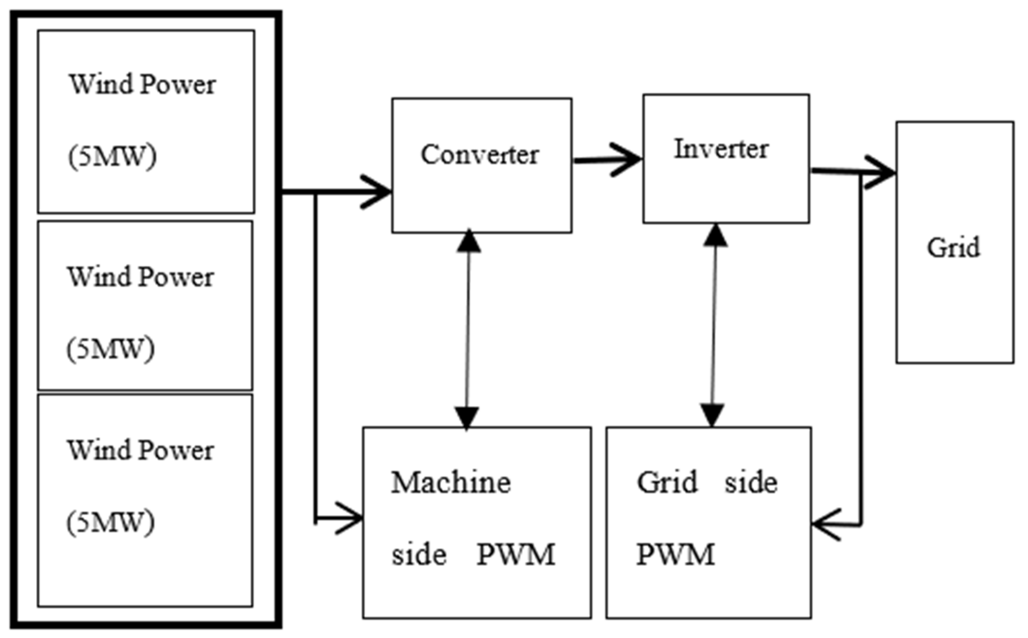
Three of the modeled DFIGs were then connected to form a wind farm and connected the grid through a rotor side PWM controller and grid side PWM controller and a transformer as depicted in
Figure 2. The power from this wind farm is injected to different buses of the grid for analysis.
3.2. Voltage Stability
Voltage stability analysis can be done by the use of time simulations that capture the events that lead to instability or by the use of static methods that examine the viability of a balance point that is represented by specified parameters of the power system. There are four static methods for voltage stability analysis: V-Q Sensitivity Analysis, Q-V Modal Analysis, V-Q Curves and P-V Curves. These methods allow investigation of several system conditions which can provide information about the nature of the problem and can identify the key causes [
16,
17].
This paper utilizes the static methods to assess the effects of connecting wind power into the grid.
3.2.1. Q-V Sensitivity Analysis
This method calculates the relationship between change in voltage and that of reactive power.
where Δ
U = vector representing incremental change in bus voltage magnitude, Δ
Q = vector representing incremental change in bus reactive power injection, and
= reduced Jacobian matrix.
The V-Q sensitivities are calculated from the elements of the inverse of the reduced Jacobian matrix
while the diagonal components are the self sensitivities which are given by:
The non-diagonal elements are the mutual sensitivities
The sensitivities of the buses whose voltages are controlled are equal to zero since their voltages are assumed to be constant. V-Q sensitivities can either be positive or negative where positive sensitivities show that the system is under stable operation, and the smaller the sensitivity, the more stable the system is. A decrease in stability leads to an increase in the magnitude of the sensitivity, becoming infinite at the stability limit. Negative sensitivities show unstable operation, and the system is uncontrollable in this region.
3.2.2. Q-V Modal Analysis
This modal analysis approach provides more information regarding the mechanism of instability. In order to identify the voltage stability characteristics of the system, the eigenvalues and eigenvectors of the reduced Jacobian matrix
are calculated [
18].
where Λ = diagonal eigenvalue matrix, ξ = right eigenvector matrix, η = left eigenvector matrix, ξ
i = the ith right eigenvector, ith column of right eigenvector matrix, and η
i = the ith left eigenvector, ith row of left eigenvector matrix.
Using modal analysis techniques Equation (9) becomes
where u = η ΔU is the vector of modal voltage variations, and q = η ΔQ is the vector of modal reactive power variations.
The inverse transformation of (13) is given by
In V-Q modal analysis, positive eigenvalue shows that the system voltage is stable with a smaller magnitude showing that the ith modal voltage is closer to being unstable. These eigenvalues’ magnitudes can give information of the nearness to instability. When the magnitude of the eigenvalue is zero, it shows that the ith modal voltage collapses because any change in that modal reactive power will lead to the modal voltage changing to infinity. A negative eigenvalue shows that the voltage in the system is unstable. Zero reactive power is assumed for buses without load elements.
Bus participation factors are used to give the relative participation of a bus in a given mode and to determine voltage weak buses that are not controllable. The sum of the magnitudes of all the bus participation factors for a given mode is equal to unity. The magnitude of bus participation in a given mode indicates how effective the mitigation actions applied at that given section of the system in stabilizing that mode are.
Branch participation factors give the relative participation of branch
in a certain mode and are given by the participation factor [
18].
The system branch participation factors are used to determine which branches consume the most reactive power in response to an increase in reactive load. Any branch with a high participation factor is either a weak link or is heavily loaded. Branch participation is important when identifying mitigation measures to solve voltage stability problems and for contingency selection.
4. Results and Discussion
Simulation was done considering two test buses: IEEE 14 bus test system and IEEE 39 bus test system.
4.1. Case I (IEEE 14 Bus Test Sytem)
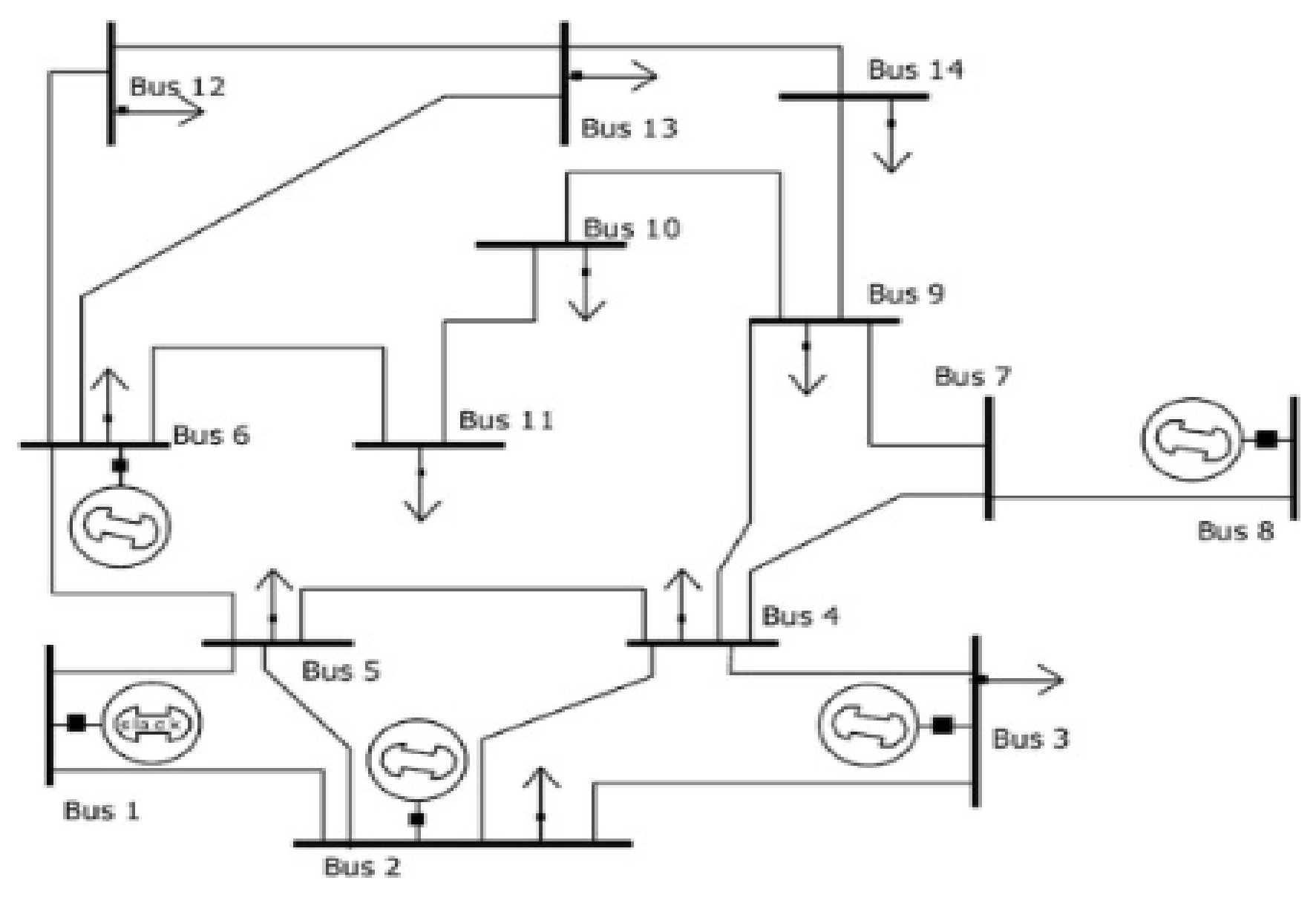
In order to test the effects of connecting wind power into the grid, the IEEE 14 bus system was used as a test bus. The wind power from the modeled DFIG generator was injected at buses 9, 10 and 14, and the effects of this power injection were analyzed. The reactive power on load 10 connected to bus 10 was varied, and the results were also analyzed. The IEEE 14 bus system used is shown in
Figure 3.
4.1.1. Voltage Profile
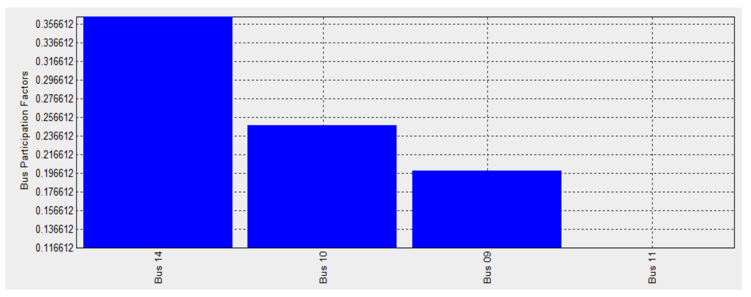
Power from the modeled wind turbine system was injected into the voltage weak buses, 9, 10 and 14 of the IEEE 14 bus system as determined by the use of bus participation factors shown in
Figure 4.
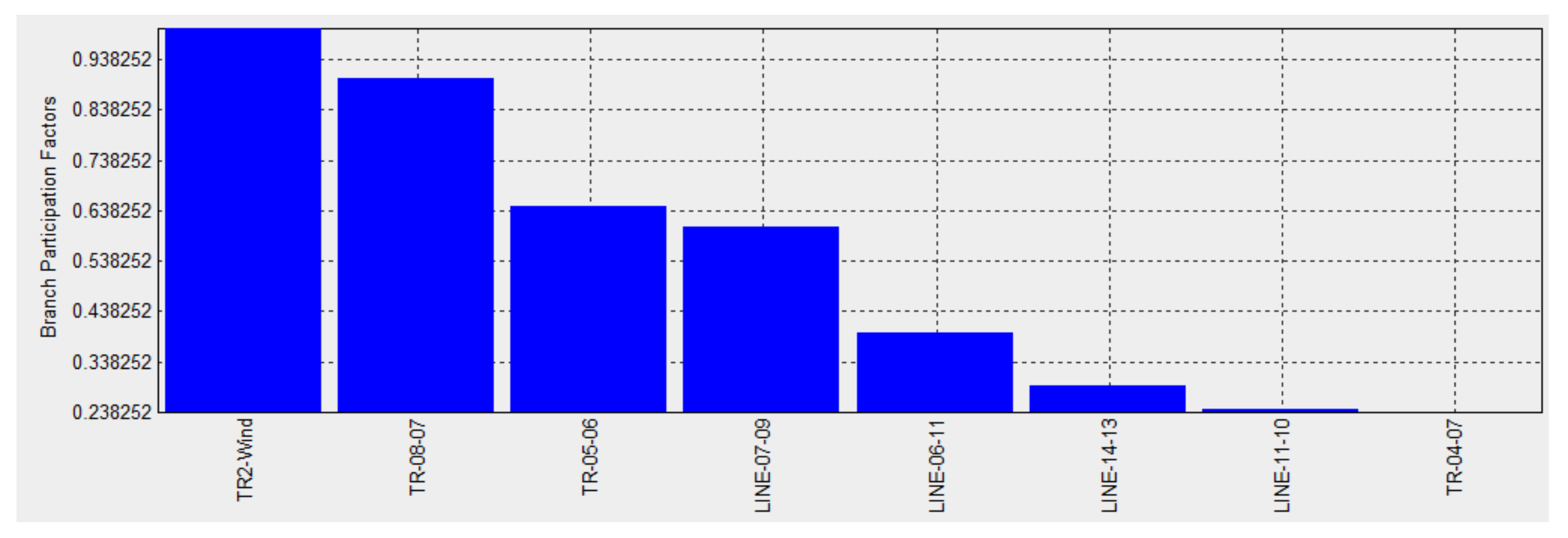
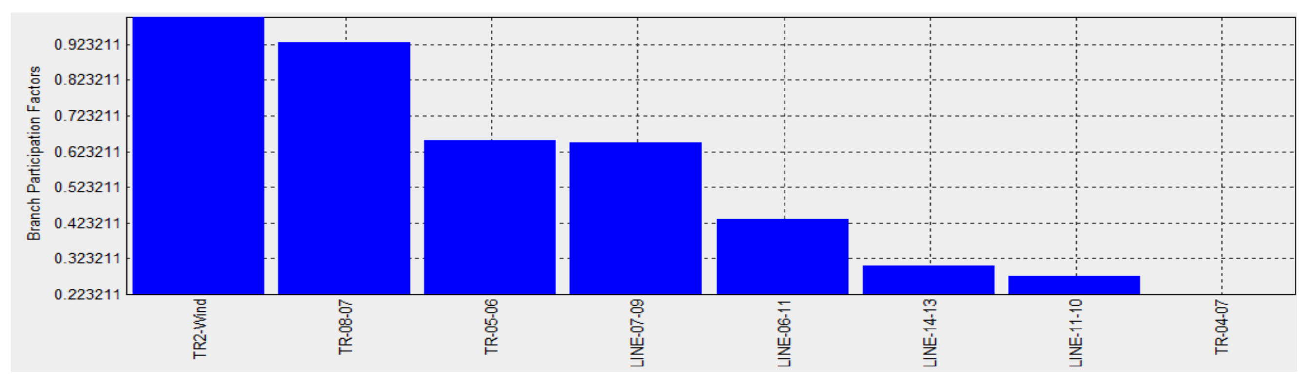
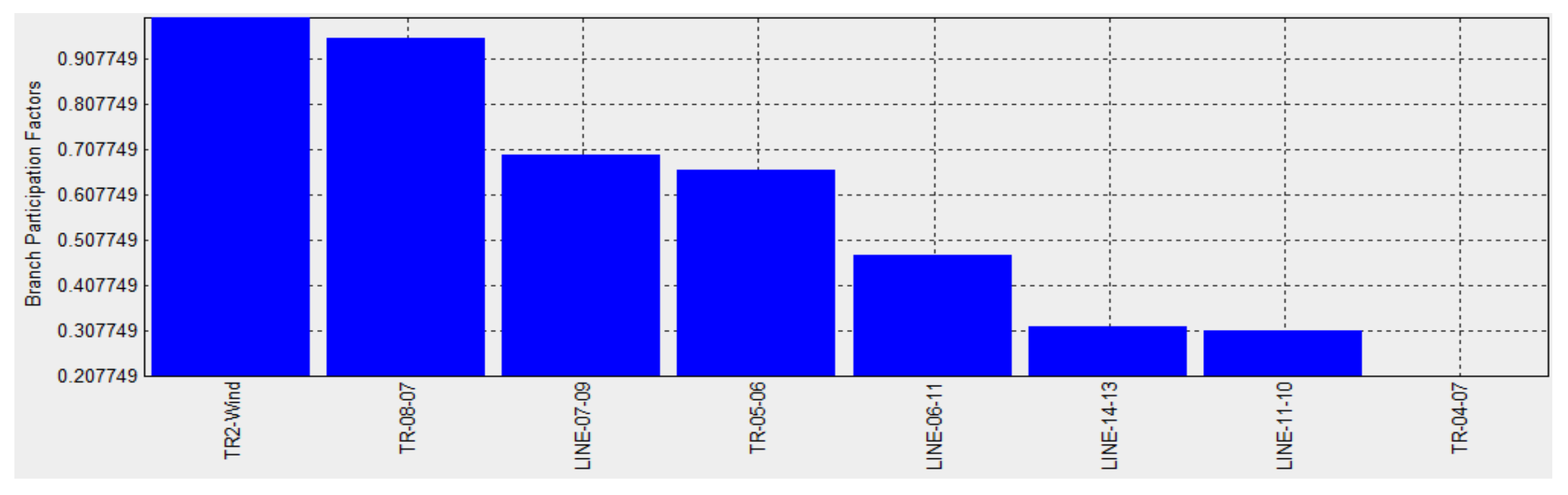
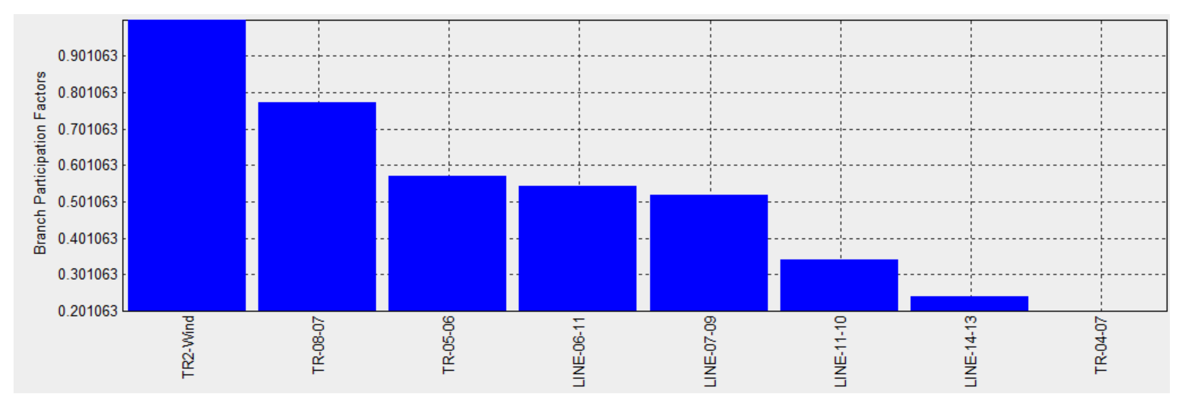
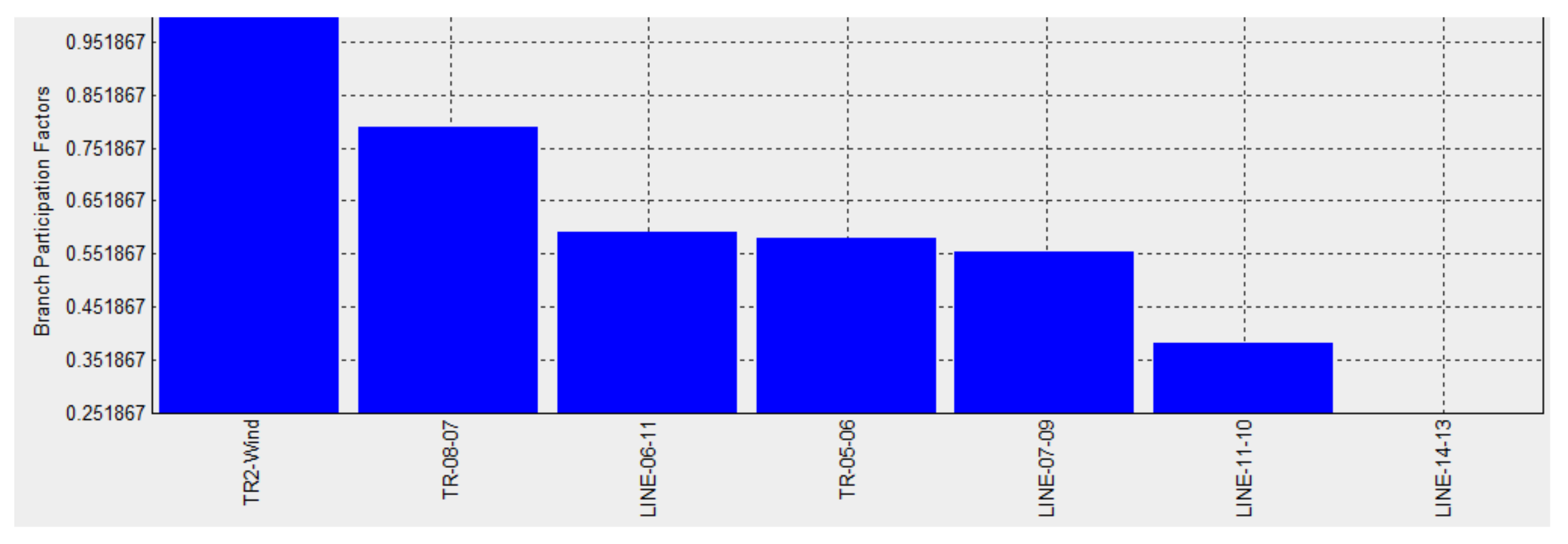
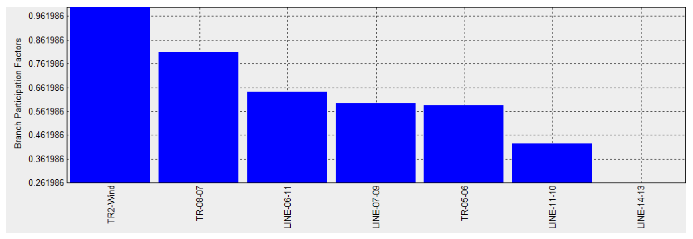
By varying the reactive power on the load at bus 10, the branch participation factors are considered to analyze which branches consume the highest reactive power for incremental reactive load at a given bus with wind energy injection. The results are shown in
Figure 5,
Figure 6,
Figure 7,
Figure 8,
Figure 9,
Figure 10,
Figure 11,
Figure 12 and
Figure 13 for wind power injections at buses 9, 10 and 14.
Injection at Bus 9
Injection at Bus 10
Injection at Bus 14
From
Figure 5,
Figure 6,
Figure 7,
Figure 8,
Figure 9,
Figure 10,
Figure 11,
Figure 12 and
Figure 13, it is noted that the branch with TR-08-07 (transformer between buses 7 and 8) consumes the highest reactive power compared to the other branches when wind power is injected at buses 9 and 10 while the branch line-14-13 consumes the highest reactive power when wind power is injected at bus 14. These are the branches that will need remedial actions so as to maintain voltage levels at expected limits.
4.1.2. Q-V Sensitivities
Q-V sensitivities were analyzed for wind power injections at buses 9, 10 and 14 as shown in
Table 2.
From
Table 2, Q-V sensitivities are highest at the B-Wind bus and bus 14 and lowest for Buses 05 and 04 for all three wind power injections at buses 09, 10 and 14.
4.1.3. Comparison of Results with Other Works
From
Table 3, references [
19,
20] found that the VQ sensitivities are highest for buses 14, 10, 12 and 11 which is similar to this paper. Furthermore, references [
19,
21,
22] found that the weakest bus was bus 14, and injection wind turbine power was done at this bus. This was one of the buses selected in this paper in addition to buses 09 and 10 to be able to have more values for assessment. Bus participation factors with highest participation were found by [
19,
20] to be buses 14, 10 and 9 with bus 14 being the highest; this is the same as those found in this paper. In addition to bus participation factors and Q-V sensitivities, branch participation factors are also considered in this paper to give more information on the effects of changing reactive power on the bus loads in a system with wind power injection.
4.2. Case II (IEEE 39 Bus System)
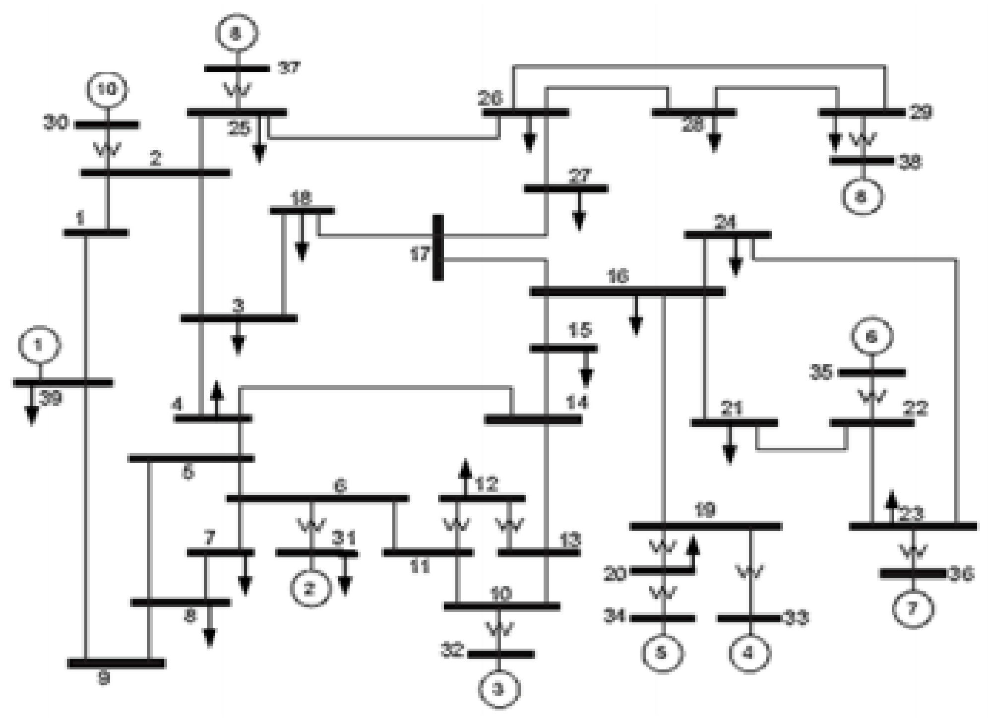
In the second case, IEEE 39 bus system shown in
Figure 14 was used to analyze the effects of wind power injection on the voltages of the system using bus participation factors, branch participation factors and Q-V sensitivities.
4.2.1. Voltage Profile
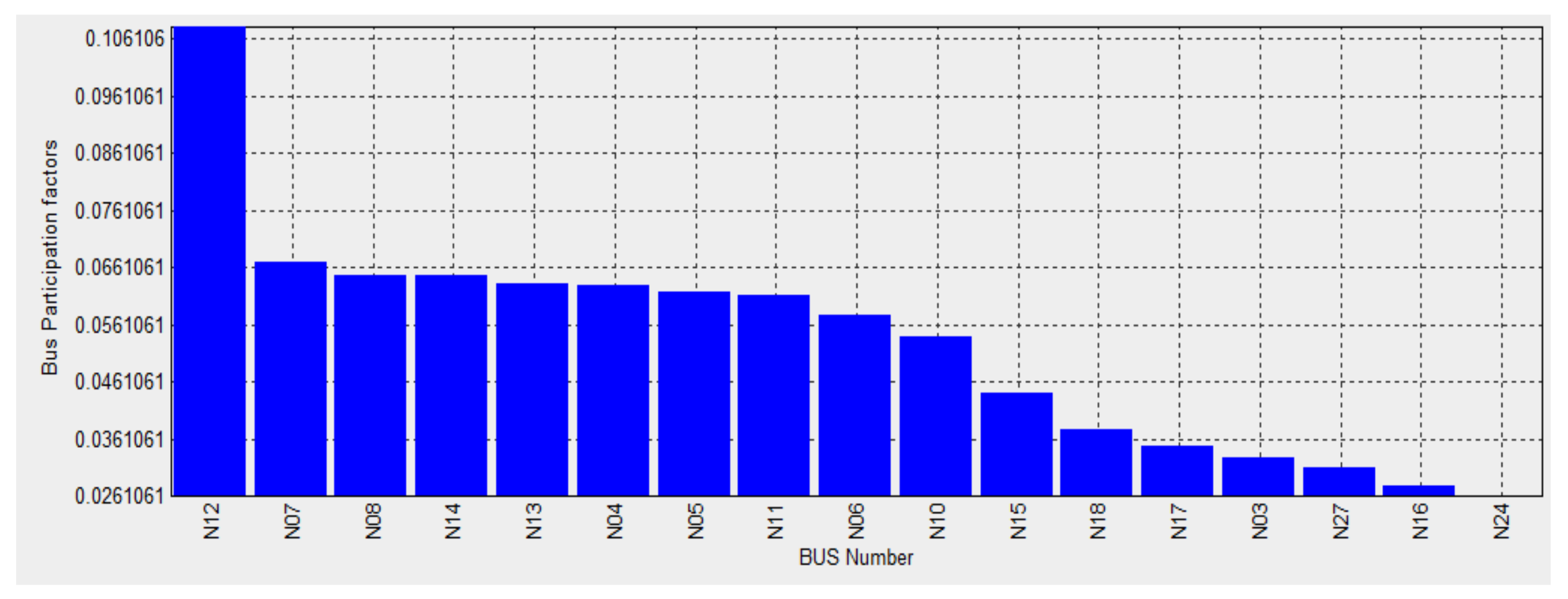
Weak buses in the IEEE 39 test bus system were determined using bus participation factors as shown in
Figure 15.
Table 4 shows the voltage profile of the system before injection of wind power and after injection of wind power for comparison purposes. It is noted that injection of wind power into the IEEE 39 bus system helps in slightly stabilizing the voltages as seen in bus 02 (from 104.87% to 104.85%), bus 03 (from 103.02% to 102.99%) and bus 04 (from 100.39% to 100.37%).
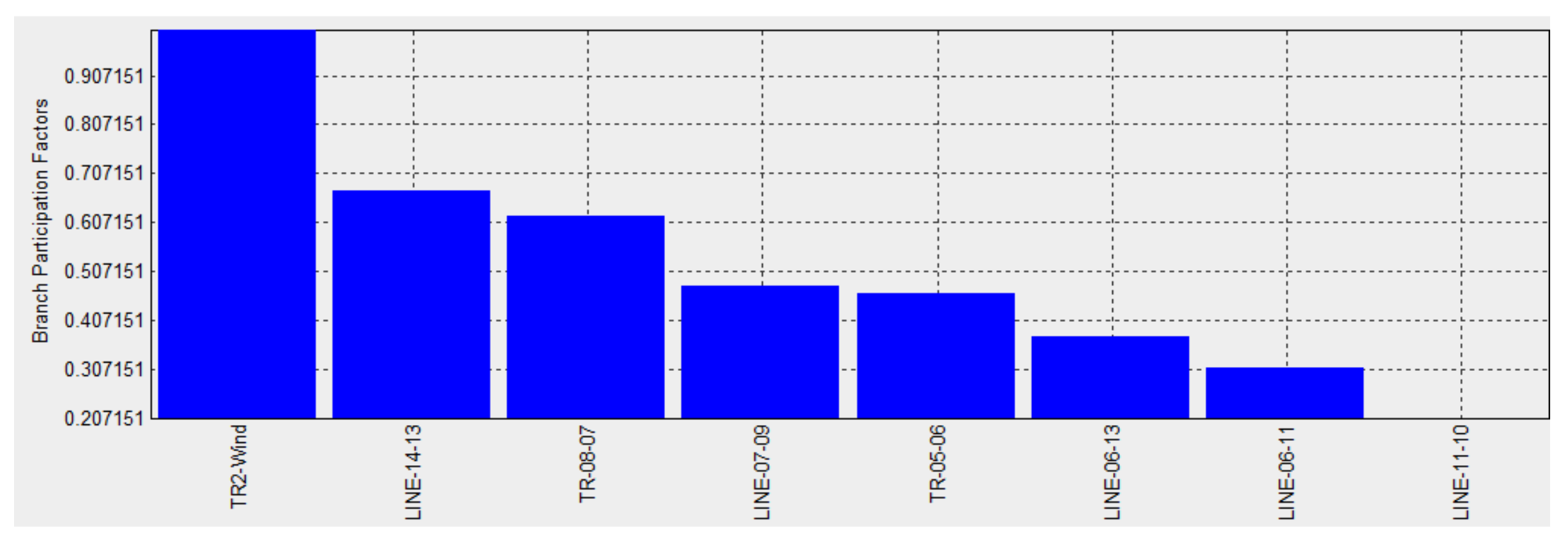
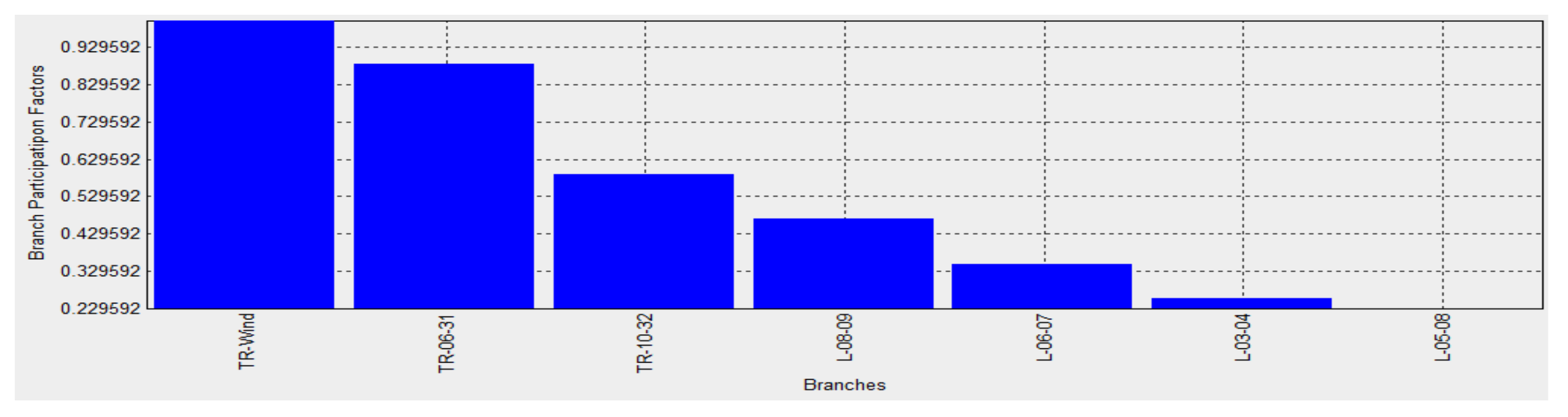
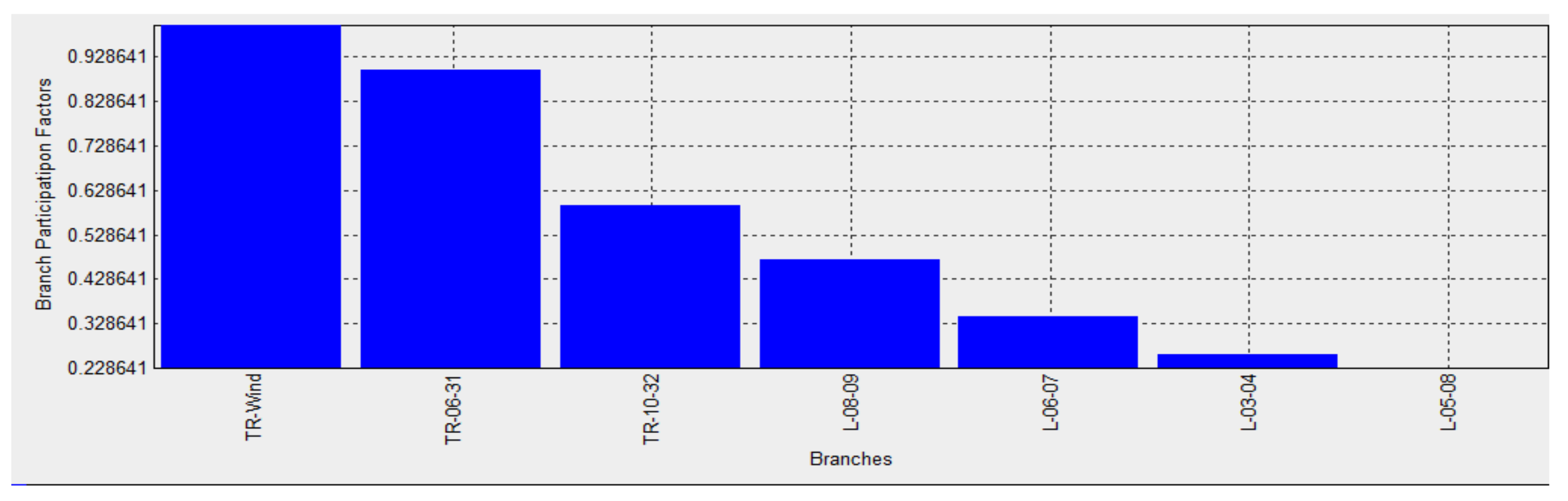
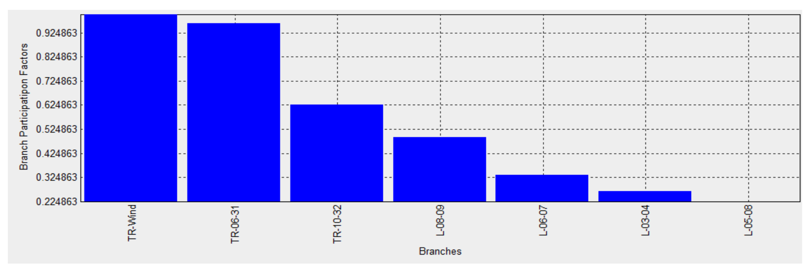
Power from the modeled wind turbine system was injected into the two weakest buses: 12 and 07 of the IEEE 39 bus system. The reactive power on the load at bus 06 was varied, and the branch participation factors were considered to analyze which branches consume the highest reactive power for incremental reactive load at a given bus with wind energy injection. The results are shown in
Figure 16,
Figure 17,
Figure 18,
Figure 19,
Figure 20 and
Figure 21.
Injection at bus 07
Injection at bus 07 with changing reactive power at bus 12
From
Figure 16,
Figure 17,
Figure 18,
Figure 19,
Figure 20 and
Figure 21, it is noted that for lower values of reactive loads on both buses 06 and 12, the wind bud (TR-Wind) consumes the highest reactive power while for higher values of reactive loads, branch TR-06-31 (line connecting buses 06 and 31) consumes the highest reactive power. These are the branches that will need remedial actions so as to maintain voltage levels at expected limits.
4.2.2. Q-V Sensitivities
Q-V sensitivities before wind power injection and after injection of wind power at buses 07 and 12 are shown in
Table 5.
From
Table 5, Q-V sensitivities remain the same when the wind power is injected at node 07 and increase from 0.0332 to 0.0333 for node 12 when wind power is injected at node 12 which is the weakest bus.
4.2.3. Comparison of Results with Other Works
Reference [
23] used V-Q and P-V curves and found out that bus 12 is the weakest bus as found from both bus participation factors and branch participation factors in this paper. Reference [
24] analyzed the voltage profile of a 33 bus system using loadability index while this paper uses V-Q sensitivities for the analysis. Reference [
25] presented that integration of wind power into a power network helps in improving the voltage stability; this paper from the voltage profile in
Table 4 also found that injection of 15 MW wind power to buses 12 and 28 helps in stabilizing the voltage levels.
5. Conclusions
This paper dealt with the modeling of the wind turbine generator (DFIG). Three of these generators were used to inject power into IEEE 14 and IEEE 39 bus test systems. Bus participation factors were used to determine the weakest buses of the networks. Branch participation factors were analyzed when the wind power was injected at the voltage weak buses with incremental changes in load reactive powers to determine unstable branches. Q-V analysis was also done for both cases to determine the buses that have high voltage sensitivities arising from the injection of wind power. From the participation factors and Q-V sensitivities, the sections of the grid where remedial measures for voltage levels were determined. The remedial devices that can be used are the Flexible AC Transmission systems (FACTSs) such as static compensators (STATCOMs) and static var compensators or the unified power flow controller (UPFC). From the simulations done, it was noted that there are specific branches that will result in instability for most of the injection cases from branch participation factors and QV sensitivities; hence mitigation equipment can be installed in these branches. Lastly, the results from this paper were compared with existing similar works in literature.
Author Contributions
Conceptualization, N.S.; methodology, N.S.; software, N.S.; validation, N.S., J.M. and L.L.; formal analysis, N.S.; investigation, N.S.; resources, N.S.; visualization, N.S.; supervision, J.M. and L.L.; project administration, N.S.; funding acquisition, N.S., J.M. and L.L. All authors have read and agreed to the published version of the manuscript.
Funding
This research was fully funded by World Bank and University of Rwanda through African Centre of Excellence in Energy and Sustainable Development, ACE-ESD.
Conflicts of Interest
The authors declare no conflict of interest.
References
- Enemuoh, F.O.; Onuegbu, J.C.; Anazia, E.A. Modal Based Analysis and Evaluation of Voltage Stability on Bulk Power System. Int. J. Eng. Res. Dev. 2013, 6, 71–79. [Google Scholar]
- Khami, M.J.; Atiyahsity, B.T.; Ashen, K.M. Computer Aided Stability Analysis in Power System. J. Thi Qar Univ. April 2010. Available online: https://www.researchgate.net/publication/332233617_Computer_Aided_Voltage_Stability_Analysis_in_Power_Systems (accessed on 22 January 2021).
- Ajjarapu, V. Computational Techniques for Voltage Stability Assessment; Springer: Berlin, Germany, 2006. [Google Scholar]
- Cutsen, T.; Vournas, C. Voltage Stability of Electric Power Systems; Springer: New York, NY, USA, 2008. [Google Scholar]
- Farhoodnea, M.; Mohamed, A.; Shareef, H.; Zayandehroodi, H. Power Quality Impact of Renewable Energy Based Generators and Electric Vehicles in Distribution Systems. In Proceedings of the 4th International Conference on Electrical Engineering and Informatics (ICEEI), Selangor, Malaysia, 24–25 June 2013; pp. 11–17. [Google Scholar]
- El-Samahy, I.; El-Saadany, E. The Effect of DG on Power Quality in a deregulated Environment. In Proceedings of the IEEE Power Engineering Society General Meeting 2005. IEEE Power Energy Mag. 2005, 3, 67. [Google Scholar] [CrossRef]
- Khadem, S.K.; Basu, M.; Conlon, M.F. Power Quality in Grid Connected Renewable Energy Systems-Role of Custom Power Devices. In Proceedings of the International Conference in Raenewable Energies and Power Quality (ICREPQ’2010), Granada, Spain, 23–25 March 2010. [Google Scholar]
- Kumar, K.S.V.P.; Venkateshwarla, S. A Review of Power Quality in Grid Connected Renewable energy system. CVR J. Sci. Technol. 2013, 5, 57–61. [Google Scholar] [CrossRef]
- Colak, I.; Fulli, G.; Bayhan, S.; Chondrogiannis, S.; Demirbas, S. Critical Aspects of Wind Energy Systems in Smart Grid Applications. Renew. Sustain. Energy Rev. 2015, 52, 155–171. [Google Scholar] [CrossRef]
- Blaabjerg, F.; Ma, K. Future on Power Electronis for Wind Turbine Systems. IEEE J. Emerg. Sel. Top Power Electron. 2013, 1, 139–152. [Google Scholar] [CrossRef]
- Jadhav, H.T.; Roy, R. Comprehensive Review on the Grid Integration of Doubly Fed Induction Generator. Electr. Power Energy Syst. J. 2013, 49, 8–18. [Google Scholar] [CrossRef]
- Jeng, F.; Chang, J. Intelligent Controlled Three-phase Squirrel-cage Induction Generator System Using Hybrid Wavelet Fuzzy Neural Network. In Proceedings of the IEEE International Conference on Fuzzy Systems, Beijing, China, 6–11 July 2014; pp. 6–11. [Google Scholar]
- Yaramasu, V.; Wu, B. Predictive Control of a Three-level Boost Converter and an NPC Inverter for High-Power PMSG-Based Medium Voltage Wind Energy Conversion Systems. IEEE Trans. Power Electron 2014, 29, 5308–5322. [Google Scholar] [CrossRef]
- Duggirala1, V.N.A.; Gundavarapu, V.N.K. Dynamic Stability Improvement of Grid Connected DFIG Using Enhanced Field Oriented Control Technique for High Voltage Ride Through. J. Renew. Energy 2015, 2015. [Google Scholar] [CrossRef]
- Wu, Y.-K.; Shu, W.-H.; Cheng, H.-Y.; Ye, G.-T.; Jiang, D.-C. Mathematical Modelling and Simulation of the DFIG-based Wind Turbine. In Proceedings of the 2014 CACS International Automatic Control Conference (CACS 2014), Kaohsiung, Taiwan, 26–28 November 2014. [Google Scholar]
- Zad, B.B.; Lobry, J.; Vallée, F. A New Voltage Sensitivity Analysis Method for Medium-Voltage Distribution Systems Incorporating Power Losses Impact. Electr. Power Compon. Syst. J. 2018, 46, 1540–1553. [Google Scholar] [CrossRef]
- Zad, A.; Hasan, H.; Lobry, J.; Vallée, F. Optimal reactive power control of DGs for voltage regulation of MV distribution systems using sensitivity analysis method and PSO algorithm. Int. J. Electr. Power Energy Syst. 2015, 68, 52–60. [Google Scholar]
- Sanchez, J.L.; Rios, M.A.; Zapata, C.J.; Gomez, O. Improved Branch participation factor in Voltage stability Assessment. Int. Rev. Modeling Simul. 2009, 2, 18–24. [Google Scholar]
- Djari, M.A.; Benasla, L.; Rahmouni, W. Voltage Stability Assessment Using the V-Q Sensitivity and Modal Analyses Methods. In Proceedings of the 5th International Conference on Electrical Engineering—Boumerdes (ICEE-B), Boumerdes, Algeria, 29–31 October 2017. [Google Scholar]
- Reddy, D.V.B. Voltage Collapse Prediction and Voltage Stability Enhancement by Using Static Var Compensator. Int. J. Eng. Res. Appl. 2013, 3, 798–805. [Google Scholar]
- Boonchiam, P.N.; Sode-Yome, A.; Mithulananthan, N.; Aodsup, K. Voltage Stability in Power Network when connected Wind Farm Generators. In Proceedings of the IEEE Xplore Conference, Wuhan, China, 11–13 December 2009. [Google Scholar]
- Kumar, S.; Kumar, A.; Sharma, N.K. A novel method to investigate voltage stability of IEEE-14 bus wind integrated system using PSAT. In Front Energy; Higher Education Press: Beijing, China; Springer: Berlin/Heidelberg, Germany, 2016. [Google Scholar]
- Upadhyay, P.A.; Joshi, S.K. Volatage stability analysis through reactive power reserve and voltage sensitivity factor. J. Sci. Eng. Res. 2014, 1, 76–84. [Google Scholar]
- Venkatesh, B.; Ranjan, R.; Gooi, H.B. Optimal reconfiguration of radial distribution systems to maximize loadability. IEEE Trans. Power Syst. 2004, 19, 260–266. [Google Scholar] [CrossRef]
- Baalbergen, J.F.; De Tommasi, L.; Gibescu, M.; Visscher, K.; Van Der Sluis, L. Consequences of offshore wind farms on voltage stability at the transmission network level. In Proceedings of the CIGRE 2011 Bologna Symposium—The Electric Power System of the Future: Integrating Supergrids and Microgrids, Bologna, Itlay, 13–15 September 2011. [Google Scholar]
Figure 1.
Schematic diagram for a grid-connected doubly-fed induction generator (DFIG) [
14].
Figure 1.
Schematic diagram for a grid-connected doubly-fed induction generator (DFIG) [
14].
Figure 2.
Grid-connected wind farm.
Figure 2.
Grid-connected wind farm.
Figure 3.
IEEE 14 Bus system.
Figure 3.
IEEE 14 Bus system.
Figure 4.
Weak buses for the IEEE 14 bus system.
Figure 4.
Weak buses for the IEEE 14 bus system.
Figure 5.
Branch participation factors with injection at bus 9 (Q at bus 10 = 8.12 MVar).
Figure 5.
Branch participation factors with injection at bus 9 (Q at bus 10 = 8.12 MVar).
Figure 6.
Branch participation factors with injection at bus 9 (when Q at bus 10 = 12 MVar).
Figure 6.
Branch participation factors with injection at bus 9 (when Q at bus 10 = 12 MVar).
Figure 7.
Branch participation factors with injection at bus 9 (when Q at bus 10 = 16 MVar).
Figure 7.
Branch participation factors with injection at bus 9 (when Q at bus 10 = 16 MVar).
Figure 8.
Branch participation factors with injection at bus 10 (when Q at bus 10 = 8.12 MVar).
Figure 8.
Branch participation factors with injection at bus 10 (when Q at bus 10 = 8.12 MVar).
Figure 9.
Branch participation factors with injection at bus 10 (when Q at bus 10 = 12 MVar).
Figure 9.
Branch participation factors with injection at bus 10 (when Q at bus 10 = 12 MVar).
Figure 10.
Branch participation factors with injection at bus 10 (when Q at bus 10 = 16 MVar).
Figure 10.
Branch participation factors with injection at bus 10 (when Q at bus 10 = 16 MVar).
Figure 11.
Branch participation factors with injection at bus 14 (when Q at bus 10 = 8.12 MVar).
Figure 11.
Branch participation factors with injection at bus 14 (when Q at bus 10 = 8.12 MVar).
Figure 12.
Branch participation factors with injection at bus 14 (when Q at bus 10 = 12 MVar).
Figure 12.
Branch participation factors with injection at bus 14 (when Q at bus 10 = 12 MVar).
Figure 13.
Branch participation factors with injection at bus 14 (when Q at bus 10 = 16 MVar).
Figure 13.
Branch participation factors with injection at bus 14 (when Q at bus 10 = 16 MVar).
Figure 14.
IEEE 39 bus system [
18].
Figure 14.
IEEE 39 bus system [
18].
Figure 15.
Weak buses for the IEEE 39 bus system.
Figure 15.
Weak buses for the IEEE 39 bus system.
Figure 16.
Branch participation factors with injection at bus 07 (when Q at bus 06 = 0.000 MVar).
Figure 16.
Branch participation factors with injection at bus 07 (when Q at bus 06 = 0.000 MVar).
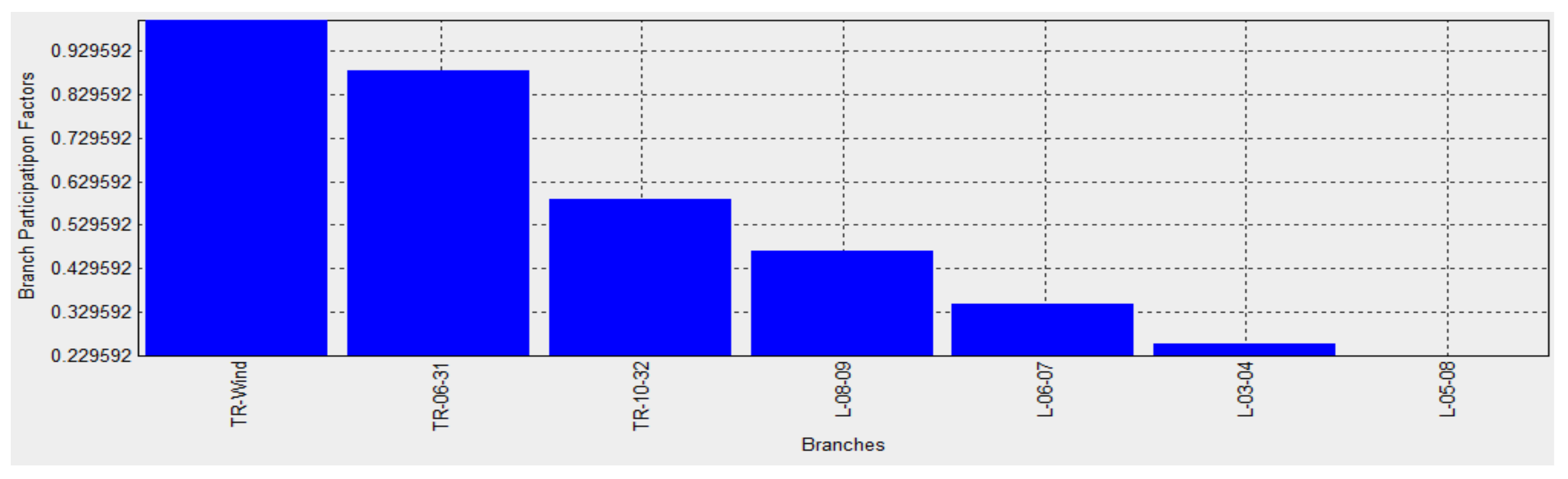
Figure 17.
Branch participation factors with injection at bus 07 (when Q at bus 06 = 10.0 MVar).
Figure 17.
Branch participation factors with injection at bus 07 (when Q at bus 06 = 10.0 MVar).
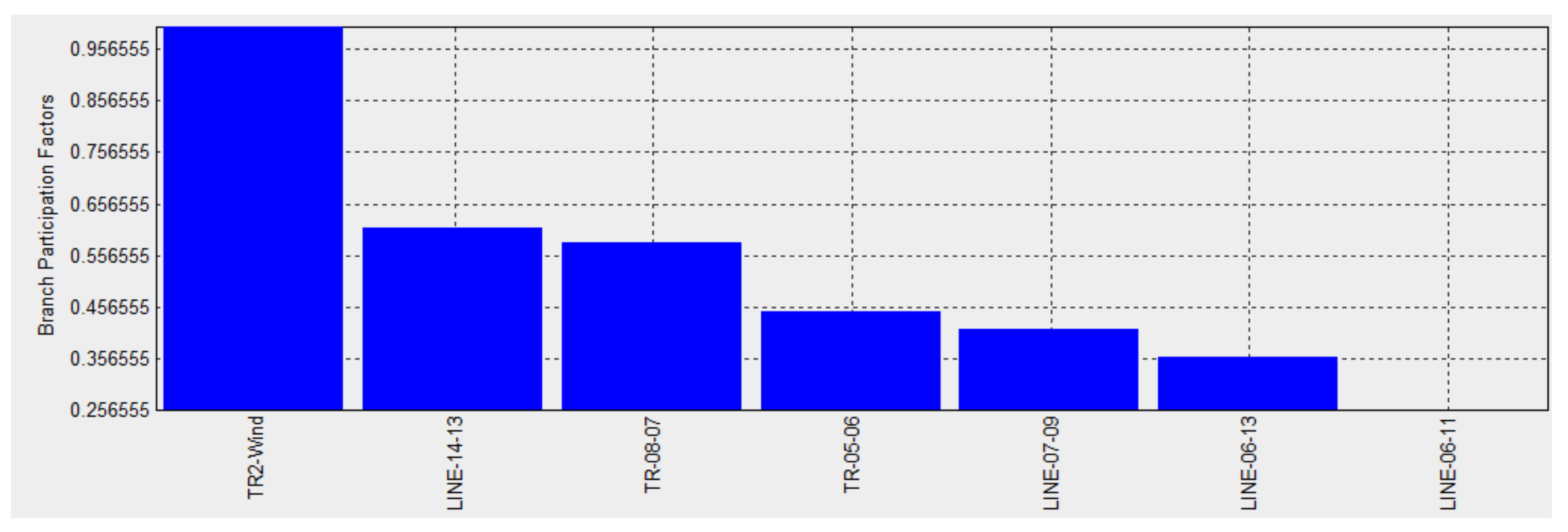
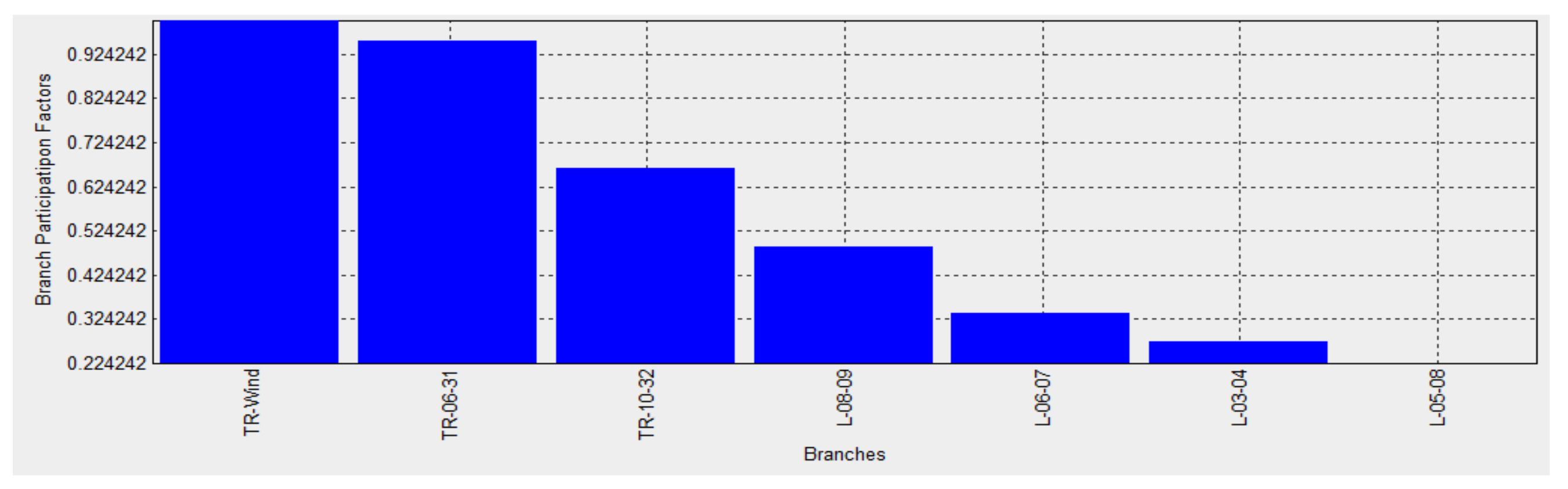
Figure 18.
Branch participation factors with injection at bus 07 (when Q at bus 06 = 50.0 MVar).
Figure 18.
Branch participation factors with injection at bus 07 (when Q at bus 06 = 50.0 MVar).
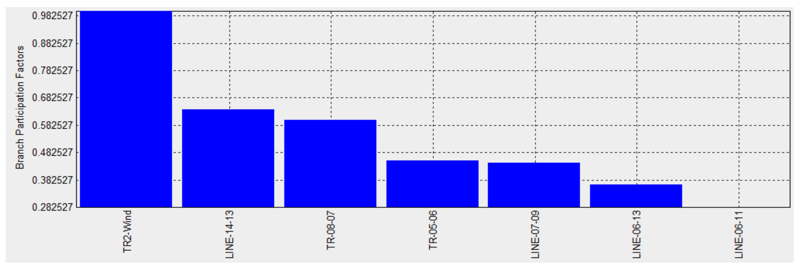
Figure 19.
Branch participation factors with injection at bus 07 (when Q at bus 12 = 88.0 MVar).
Figure 19.
Branch participation factors with injection at bus 07 (when Q at bus 12 = 88.0 MVar).
Figure 20.
Branch participation factors with injection at bus 07 (when Q at bus 12 = 100.0 MVar).
Figure 20.
Branch participation factors with injection at bus 07 (when Q at bus 12 = 100.0 MVar).
Figure 21.
Branch participation factors with injection at bus 07 (when Q at bus 12 = 150.0 MVar).
Figure 21.
Branch participation factors with injection at bus 07 (when Q at bus 12 = 150.0 MVar).
Table 1.
DFIG machine parameters.
Table 1.
DFIG machine parameters.
| Parameter | Value |
|---|
| Power | 5 MW |
| Voltage | 3.3 kV |
| Frequency | 50 Hz |
| Speed | 1494.2 rev/min |
| Power factor | 0.85498 |
| Slip | 0.388 |
| Efficiency | 0.99 |
| Pole pairs | 2 |
Table 2.
Q-V sensitivities for wind power injection at bus 9.
Table 2.
Q-V sensitivities for wind power injection at bus 9.
| Q-V Sensitivities |
|---|
| Bus Number | Injection at Bus 9 | Injection at Bus 10 | Injection at Bus 14 |
|---|
| % MVar | % MVar | % MVar |
|---|
| B-Wind | 1.0858 | 1.1215 | 1.2093 |
| Bus 14 | 0.2181 | 0.2180 | 0.2188 |
| Bus 10 | 0.1458 | 0.1464 | 0.1455 |
| Bus 12 | 0.1387 | 0.1387 | 0.1386 |
| Bus 11 | 0.1318 | 0.1319 | 0.1318 |
| Bus 09 | 0.1116 | 0.1113 | 0.1111 |
| Bus 13 | 0.0878 | 0.0878 | 0.0877 |
| Bus 05 | 0.0421 | 0.0421 | 0.0421 |
| Bus 04 | 0.0414 | 0.0414 | 0.0414 |
Table 3.
Comparison of V-Q sensitivities.
Table 3.
Comparison of V-Q sensitivities.
| Bus Number | This Paper | V-Q for [19] | V-Q for [20] |
|---|
| 04 | 0.0416 | 0.0403 | 0.0437 |
| 05 | 0.0423 | 0.0411 | 0.0446 |
| 09 | 0.1112 | 0.1070 | 0.1029 |
| 10 | 0.1457 | 0.1548 | 0.1369 |
| 11 | 0.1319 | 0.1290 | 0.1285 |
| 12 | 0.1387 | 0.1372 | 0.1422 |
| 13 | 0.0878 | 0.0863 | 0.0869 |
| 14 | 0.2182 | 0.2186 | 0.2085 |
Table 4.
Voltage profile of IEEE 39 bus system before and after wind power integration.
Table 4.
Voltage profile of IEEE 39 bus system before and after wind power integration.
| Bus No. | Before Penetration | After Wind Integration |
|---|
| T | V | %V | V | %V |
|---|
| N01 | 10.474 | 104.74 | 10.472 | 104.72 |
| No2 | 10.487 | 104.87 | 10.485 | 104.85 |
| N03 | 10.302 | 103.02 | 10.299 | 102.99 |
| N04 | 10.039 | 100.39 | 10.037 | 100.37 |
| N05 | 10.053 | 100.53 | 10.053 | 100.53 |
| N06 | 10.077 | 100.77 | 10.077 | 100.77 |
| N07 | 9.97 | 99.7 | 9.97 | 99.7 |
| N08 | 9.96 | 99.6 | 9.96 | 99.6 |
| N09 | 10.282 | 102.82 | 10.282 | 102.82 |
| N10 | 10.172 | 101.72 | 10.17 | 101.7 |
| N11 | 10.127 | 101.27 | 10.126 | 101.26 |
| N12 | 10.002 | 100.02 | 9.996 | 99.96 |
| N13 | 10.143 | 101.43 | 10.142 | 101.42 |
| N14 | 10.117 | 101.17 | 10.116 | 101.16 |
| N15 | 10.154 | 101.54 | 10.152 | 101.52 |
| N16 | 10.318 | 103.18 | 10.316 | 103.16 |
| N17 | 10.336 | 103.36 | 10.334 | 103.34 |
| N18 | 10.309 | 103.09 | 10.307 | 103.07 |
| N19 | 10.499 | 104.99 | 10.498 | 104.98 |
| N20 | 9.912 | 99.12 | 9.911 | 99.11 |
| N21 | 10.318 | 103.18 | 10.317 | 103.17 |
| N22 | 10.498 | 104.98 | 10.497 | 104.97 |
| N23 | 10.448 | 104.48 | 10.447 | 104.47 |
Table 5.
Q-V sensitivities for IEEE 39 bus system before wind power injection, after injection at bus 07 and after injection at bus 12.
Table 5.
Q-V sensitivities for IEEE 39 bus system before wind power injection, after injection at bus 07 and after injection at bus 12.
| Q-V Sensitivities |
|---|
| | Before Wind Power Injection | After Wind Power Injection at Bus 07 | After Wind Power Injection at Bus 12 |
|---|
| Bus No. | %MVar | %MVar | %MVar |
|---|
| B-Wind | - | 1.0025 | 1.0194 |
| N12 | 0.0332 | 0.0332 | 0.0333 |
| N28 | 0.0215 | 0.0215 | 0.0215 |
| N27 | 0.0175 | 0.0175 | 0.0175 |
| N09 | 0.0170 | 0.0170 | 0.0170 |
| N01 | 0.0161 | 0.0161 | 0.0161 |
| N26 | 0.0156 | 0.0156 | 0.0156 |
| N07 | 0.0150 | 0.0150 | 0.0150 |
| N08 | 0.0146 | 0.0146 | 0.0146 |
| N15 | 0.0138 | 0.0138 | 0.0138 |
| N18 | 0.0135 | 0.0135 | 0.0135 |
| N21 | 0.0128 | 0.0128 | 0.0128 |
| N29 | 0.0126 | 0.0126 | 0.0126 |
| N14 | 0.0126 | 0.0126 | 0.0126 |
| N04 | 0.0125 | 0.0125 | 0.0125 |
| N24 | 0.0122 | 0.0122 | 0.0122 |
| N13 | 0.0120 | 0.0120 | 0.0120 |
| N11 | 0.0113 | 0.0113 | 0.0113 |
| N03 | 0.0113 | 0.0113 | 0.0113 |
| Publisher’s Note: MDPI stays neutral with regard to jurisdictional claims in published maps and institutional affiliations. |
© 2021 by the authors. Licensee MDPI, Basel, Switzerland. This article is an open access article distributed under the terms and conditions of the Creative Commons Attribution (CC BY) license (https://creativecommons.org/licenses/by/4.0/).


