Optimized Extreme Learning Machine-Based Main Bearing Temperature Monitoring Considering Ambient Conditions’ Effects

Abstract

Wind Turbines (WTs) are exposed to harsh conditions and can experience extreme weather, such as blizzards and cold waves, which can directly affect temperature monitoring. This paper analyzes the effects of ambient conditions on WT monitoring. To reduce these effects, a novel WT monitoring method is also proposed in this paper. Compared with existing methods, the proposed method has two advantages: (1) the changes in ambient conditions are added to the input of the WT model; (2) an Extreme Learning Machine (ELM) optimized by Genetic Algorithm (GA) is applied to construct the WT model. Using Supervisory Control and Data Acquisition (SCADA), compared with the method that does not consider the changes in ambient conditions, the proposed method can reduce the number of false alarms and provide an earlier alarm when a failure does occur.

1. Introduction

Since wind energy is renewable and pollution-free, many governments cite wind energy as a primary future energy source [1]. However, the high maintenance costs of Wind Turbines (WTs) seriously restrict the development of the wind energy industry [2]. The most effective way to reduce maintenance costs is to monitor the working state of WTs to sound alarms when failures occur. Thus, model-based WT monitoring has attracted widespread attention, and different methods have been proposed. Existing model-based WT monitoring methods can be roughly divided into two categories [3]: theoretical and data-driven. The advantage of theoretical methods is that fewer data are required. Reference [4] focused on the main physical mechanisms responsible for temperature changes. Reference [5] proposed an advanced annual energy computation model.

However, WTs are complex electromechanical systems, and the relationships between the various parameters are primarily nonlinear; thus, the construction of a theoretical model is difficult and often inaccurate [6]. Reference [7] proposed an approach that identifies turbines with weakened power generation performance through assessing the wind power curve profiles. Reference [8] discussed the short-horizon prediction of wind speed and power. Reference [9] used sophisticated models to understand the complex WT component degradation processes and to facilitate maintenance decision-making. Reference [10] proposed a robust data-driven fault detection approach. For data-driven methods, model accuracy relies on the quality and quantity of the data. A Supervisory Control and Data Acquisition (SCADA) system, which can record electrical parameters (active power, phase current, etc.), temperature parameters (main bearing temperature, generator rotor temperature, etc.), and operating parameters (motor speed, etc.), has been widely applied in wind farms [11,12,13].With hardware improvements, the abilities of SCADA are increasing, making the data-driven methods more suitable for WT monitoring [14].

A typical data-driven WT monitoring method analyzes real-time data using a model with one parameter as the output and other parameters as inputs [15]. When building data-driven models, intelligent algorithms are applied. By using Nonlinear State Estimate Technology (NSET), Reference [16] and Reference [17] built a tower vibration model and gearbox oil temperature model, respectively. Based on logistic regression (LR), Reference [18] and Reference [19] analyzed the direct-drive wind power generation set and the bearing performance condition, respectively. With Support Vector Machine (SVM), Reference [19] classified and diagnosed the possible fault of the bearing of WT. Reference [20] optimized SVM for Wind Turbine fault diagnosis based on a diagonal spectrum and clustering binary tree. Reference [21] presented a multi-sensory system for fault diagnosis using SVM. Reference [22] presented a two-stage fault detection and classification scheme for electric motor drives in Wind Turbine pitch systems using SVM. In addition to the above methods, Neural Network (NN) is widely applied due to its high accuracy and short training time. Reference [23] achieved a robust simultaneous estimate of actuator faults and system states using NN. Reference [24] applied an artificial NN approach to the gearbox bearings. Reference [25] improved NN by mapping the original samples into feature vectors in an embedding space. With NN, Reference [26] identified the wavelet-transformed power components’ open-circuit faults accurately. Reference [27] captured dynamic equations modeling wind power output, vibration of the drive train, and vibration of the tower. Reference [28] attempted to assess the prediction intervals of time-series predictions with NN and Extreme Learning Machine (ELM).

Since SCADA of wind farms can obtain very large datasets, NN would entail high computational costs [29]. In contrast to NN, the input weights and hidden layer biases in ELM are assigned randomly, and the output weights of the hidden layer are directly calculated by a Moore–Penrose (MP) generalized inverse operation [30,31,32]. Consequently, ELM is more computationally efficient than NN [33]. However, the ELM model is based on one set of initial weights and biases, which are mostly random. With the randomness of the initial coefficients and large quantity of datasets, the model may easily fall into local minima.GA is a global random search optimization algorithm based on the genetic mechanism and evolution. Through genetic operations, the individuals with good fitness are selected. With the strong global search capability, the initial coefficients can be optimized by GA and the solution can avoid local minima [34]. Reference [35] improved the accuracy and efficiency of a prediction algorithm by adopting the Genetic Algorithm.

Another issue is that a WT is typically exposed to harsh field conditions year-round, including extreme weather (blizzards, cold waves, etc.). Different ambient conditions have different influences on the WT’s temperature parameters. On one hand, the extreme weather causes the internal temperature to fluctuate, which can easily trigger a false alarm. On the other hand, the internal temperature shows a difference in the same normal working state due to the change in ambient temperature. For example, the ambient temperature difference can reach 50 °C between summer noon and winter midnight in the wind farm studied in this paper. Due to this huge ambient temperature difference, the main bearing temperature of a WT can differ by 20 °C in a normal working state. If the WT temperature model is constructed without considering the ambient temperature, the model can be inaccurate, which would easily cause false alarms in a normal working state, or fail to sound alarms when the internal temperature is abnormal.

Furthermore, many studies have confirmed that the WT performance is directly related to wind speed conditions [36], and thus WTs’ internal temperature parameters [37]. Therefore, it is necessary to consider the wind speed conditions in WT monitoring. In existing studies, the wind speed condition division is primarily based on the absolute value of the wind speed. This type of division is effective for WT power monitoring but not accurate for WT temperature monitoring. Through research on real data, the internal temperature is found to exhibit certain differences when wind speeds increase and decrease. For example, the temperature difference in the same main bearing between a wind speed increase and decrease may be more than 5 °C under the same wind speed of 10m/s and the same ambient temperature of 15 °C. If the wind speed condition only depends on the absolute value, the temperature monitoring result may be inaccurate.

To address these issues, a novel WT monitoring method is proposed in this paper. Considering the effects of ambient conditions on the WT’s internal temperature, the ambient temperature and wind speed change are used as inputs in the optimized ELM model, along with other related parameters. The model is developed by training with real SCADA data. The WT monitoring is achieved by analyzing the real-time data with the model.

In general, the primary innovations of this paper are as follows:

• The effects of ambient conditions (ambient temperature and wind speed change) on a WT’s internal temperature are investigated.
• Changes in the ambient conditions are used as the input of the WT temperature model. To our knowledge, this study is the first to use wind speed change as the input of a WT model.
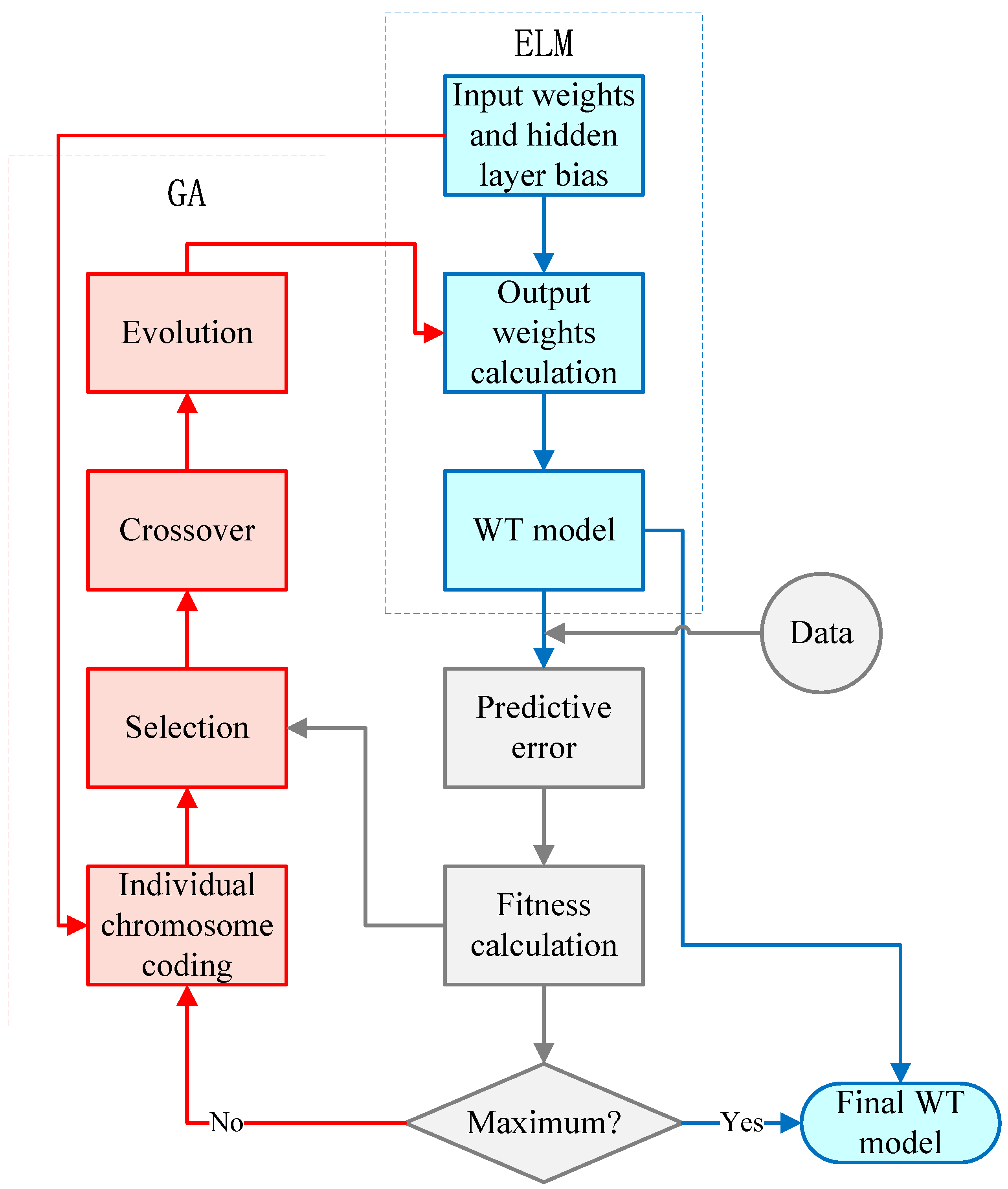
• GA is used to optimize ELM to avoid local minima due to the irregularity of initial input weights and hidden layer bias.

The rest of this paper is organized as follows. Section 2 investigates the influence of ambient conditions on WT monitoring. In Section 3, the framework of the proposed method is presented in detail. In Section 4, the WT model is developed and verified. Section 5 presents the case study and the monitoring results of various analyses. Conclusions are summarized in Section 6.

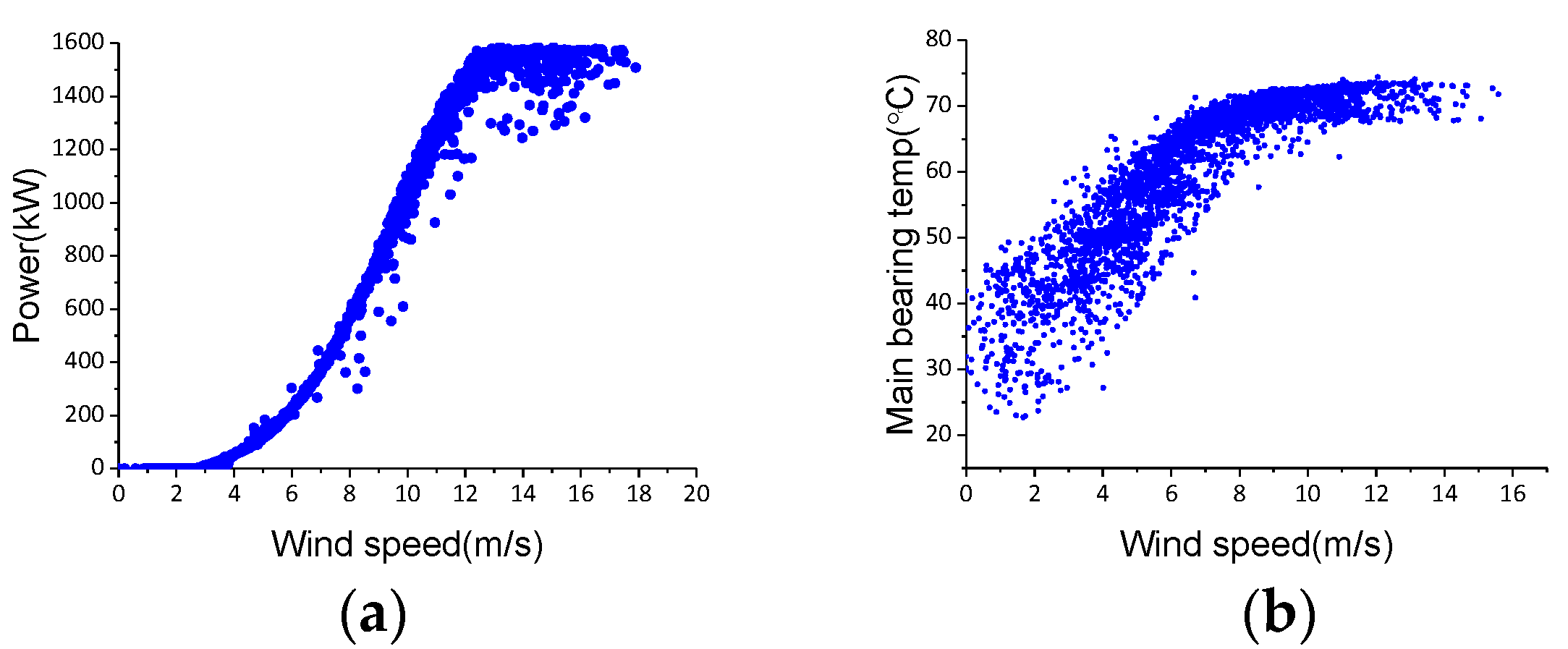
2. Effects of Ambient Conditions

A WT is a complex electromechanical system with many subsystems and components (gearbox, generator and converter, etc. [27]), and every key component has a temperature sensor. However, a WT is exposed to harsh weather conditions year-round and the ambient conditions of a WT can be very different. This huge difference in the ambient conditions can cause the internal temperatures to perform quite differently, even under the same working state. Therefore, the effects of the ambient conditions on the internal temperatures must be investigated. This paper investigates wind speed changes and ambient temperature. The data in this paper come from the Damianshan Wind Farm in Wanyuan City, Sichuan Province, China. The wind farm has a total of 33 1.5MW-WTs, with an annual power of 90.489 million kWh. The SCADA in this wind farm records data every 1 min.

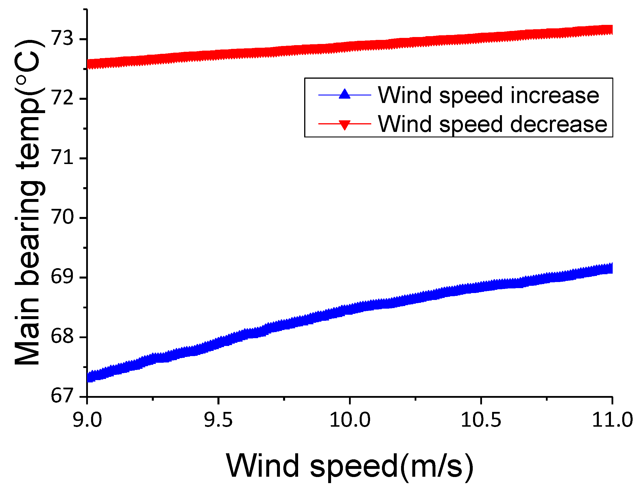
2.1. Wind Speed Change

Figure 1a shows the active power–wind speed curve under a normal working state, and Figure 1b shows the main bearing temperature–wind speed curve. To reduce the impact of the ambient temperature, the ambient temperature of the two datasets shown in the two curves is between 14.5 °C and 15.5 °C.

Figure 1a shows that the active power is directly related to the wind speed. Therefore, WT temperature monitoring should consider wind speed. Most existing methods only divide the absolute value of wind speed into three regions, (0–3, 3–12, and ≥12) m/s, without considering wind speed change. However, the fact is that wind speed change also affects the internal temperatures.

Figure 1b shows that the main bearing temperature increases as the wind speed increases; this result occurs because wind speed has a direct positive correlation with rotor speed, which is directly related to the heat generated inside. Considering the progress of the heat conduction, there may be some delay between the wind speed change and internal temperature change. Due to this delay, at the same wind speed, the main bearing temperature during a wind speed increase is smaller than during a wind speed decrease. Figure 2 shows the main bearing temperature–wind speed curve of a WT during a wind speed increase and decrease. To accurately describe this phenomenon, despite the wind speed change, the working state and conditions are similar, which are an active power of 900–1000 kW, an ambient temperature of 14–16 °C, and a wind speed of 9–11 m/s.

Figure 2 shows that, under the same wind speed, the main bearing temperature experiences a significant difference during a wind speed increase and decrease. The average difference is 4.6 °C, and the maximum difference can reach 5.4 °C. These results indicate that wind speed change affects the internal temperatures. Therefore, in order to improve the accuracy of WT monitoring, it is necessary to consider not only the absolute value of the wind speed but also the wind speed change as one of the ambient conditions.

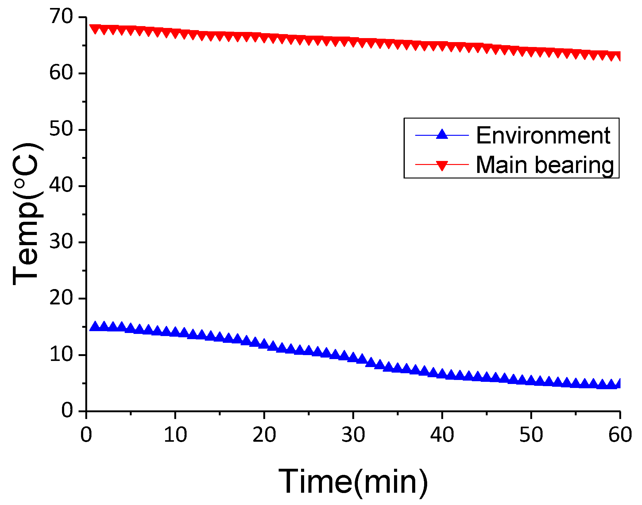
2.2. Ambient Temperature Change

Besides wind speed change, ambient temperature may also directly affect the internal temperature. Figure 3 shows the main bearing temperature of a WT at midnight (2:00–3:00 a.m.) in January (winter) and during the afternoon (14:00–15:00 p.m.) in August (summer). It is worth mentioning that, to enable effective comparison, the wind speed during the two periods was maintained at around 15m/s.

As shown in Figure 3, the difference in ambient temperature between winter and summer can reach 50.6 °C. Due to this ambient temperature difference, the average difference in the main bearing temperature is 19.2 °C. The internal temperature of the WT may change with the ambient temperature.

Additionally, extreme weather may cause large fluctuations in internal temperature in a short time. Figure 4 shows the main bearing temperature changes in one hour during a cold wave in November. During this cold wave, the WT maintains normal full-load power generation.

Figure 4 shows that the ambient temperature undergoes a significant drop of 10.2 °C due to the cold wave and the main bearing temperature undergoes a drop of 4.4 °C. The internal temperature may fluctuate due to extreme weather. Therefore, temperature monitoring must consider the ambient temperature change.

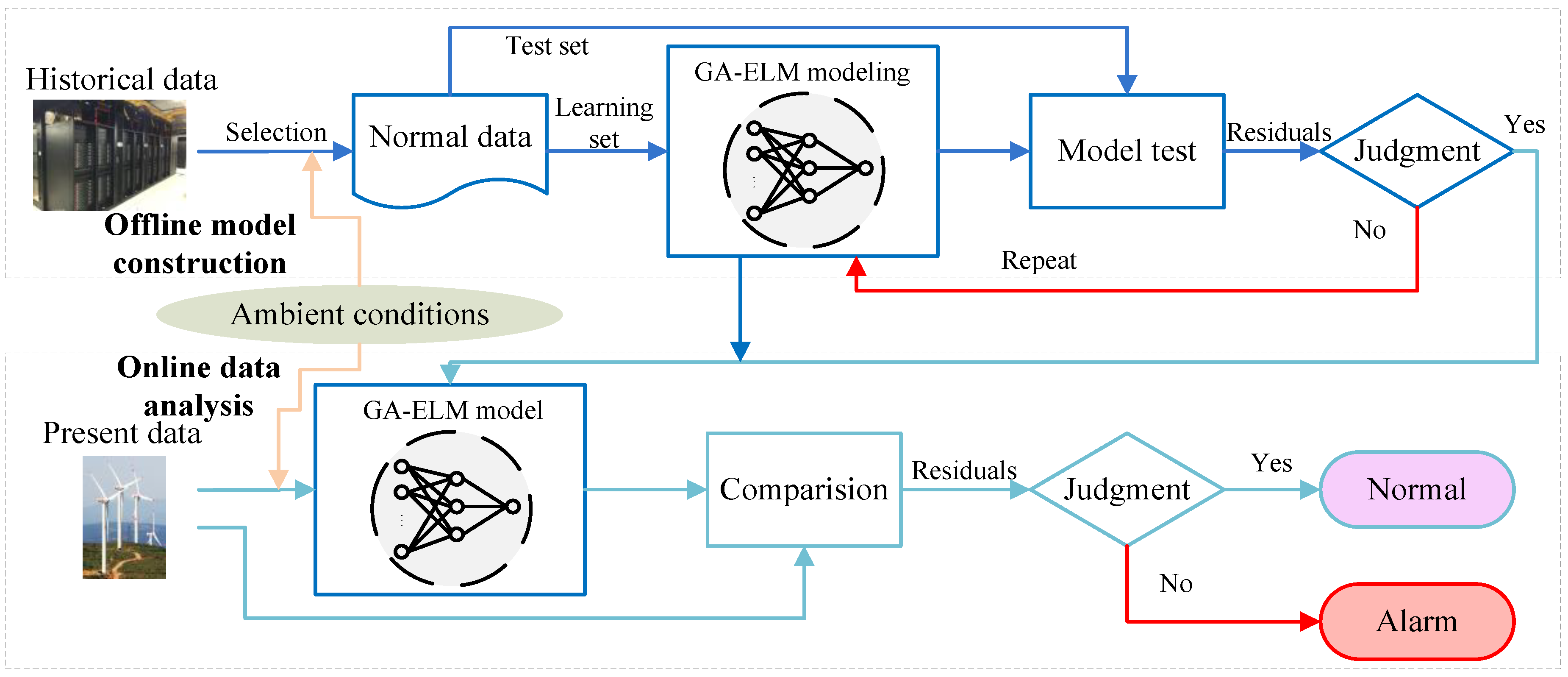
3. WT Monitoring Framework

3.1. Overview of the Proposed Framework

To address the issues noted above, a novel WT monitoring method is proposed in this paper. The framework of the proposed method is shown in Figure 5. The monitoring process is composed of two parts: offline model construction and online data analysis. Offline model construction is to build a model that simulates normal WT behaviors, and online data analysis determines whether the WT is in a normal working state.

Compared with existing methods, the proposed method has two key advantages.

Ambient conditions are used as the input of the WT model. As mentioned earlier, both wind speed change and ambient temperature affect internal temperatures. Therefore, the proposed method uses wind speed change and ambient temperature as ambient conditions in the model input.

ELM is optimized for the randomness of initial weights and bias. Due to the randomness of initial coefficients, ELM may fall into local minima when constructing the WT model. To solve this problem, GA is applied to optimize the ELM to improve the model’s accuracy.

3.2. Input Parameter Selection

The output of the model should directly describe the WT’s working state and have a strong impact on maintenance. Among the various WT failures, the main bearing failure costs the most [18]. Because the main bearing temperature is closely related to the health of the main bearing, the main bearing temperature is chosen as the output of the model in this paper.

The input should be directly related to the main bearing and WT, which are: a) the production parameters, such as active/reactive power; b) the parameters that are near the main bearing temperature, such as gearbox front/rear bearing temperature; and c) ambient conditions. In this study, the input of the model contains 10 parameters: active power, rotor speed, gearbox front bearing temperature, gearbox rear bearing temperature, nacelle ambient temperature, tower vibration, ambient temperature, ambient temperature change, wind speed, and wind speed change.

3.3. GA-ELM Modeling

The intelligent algorithm in model construction is the key to WT temperature monitoring. Compared with NN, Extreme Learning Machine (ELM) has the advantages of fast training speed and high accuracy. ELM is composed of a single hidden layer feed-forward Neural Network.

In ELM, $\mathit{X}={\left[X_1, X_2, \dots ,X_n\right]}^T\in R^n$ and $\mathit{Y}={\left[Y_1, Y_2, \dots ,Y_m\right]}^T\in R^m$ are the input and output of the model, respectively; ${\omega }_{ij}$ and ${\omega }_{ij}$ are the input and output weights, respectively. For n distinct samples X, the ELM can approximate the target as

$$\widehat{Y_k}={\displaystyle \sum }_{i=1}^{\tilde{n}}{\omega }_{jk}·g\left({\omega }_{ij}·X_i+b_i\right) j=1,2, \dots , \tilde{n}$$

(1)

where $g\left(·\right)$ represents the activation function, $\tilde{n}$ is the number of hidden nodes, and $b_i$ is the hidden layer bias.

If ELM can fit n distinct samples with zero error, the matrix form of approximation can be expressed as

$$\mathit{Y}=\widehat{\mathit{Y}}=\mathit{H}{\mathbf{\omega }}_{\tilde{n}m}$$

(2)

where the output weights ${\mathbf{\omega }}_{\tilde{n}m}={\left[{\mathbf{\omega }}_1^T,{\mathbf{\omega }}_2^T, \dots ,{\mathbf{\omega }}_m^T\right]}^T$, ${\mathbf{\omega }}_k={\left[{\omega }_{1k},{\omega }_{2k}, \dots ,{\omega }_{\tilde{n}k}\right]}^T$ and the hidden layer output matrix $\mathit{H}$can be expressed as

$$\mathit{H}={\left[\begin{array}{ccc}g\left({\omega }_{11}·X_1+b_1\right)& \dots & g\left({\omega }_{\tilde{n}1}·X_1+b_n\right)\\ \dots & \dots & \dots \\ g\left({\omega }_{1m}·X_m+b_1\right)& \dots & g\left({\omega }_{\tilde{n}m}·X_m+b_{\tilde{n}}\right)\end{array}\right]}_{m\times \tilde{n}}$$

(3)

With given input weights ${\omega }_{ij}$ and hidden layer bias $b_j$, the output weight can be analytically calculated by a least squares method as

$$\Vert \mathit{H}{\widehat{\mathit{\omega }}}_{\tilde{n}m}-\mathit{Y}\Vert = \Vert \mathit{H}{\mathit{H}}^{+}\mathit{Y}-\mathit{Y}\Vert = \underset{{\mathbf{\omega }}_{\tilde{n}m}}{\min }\Vert \mathit{H}{\mathbf{\omega }}_{\tilde{n}m}-\mathit{Y}\Vert$$

(4)

where ${\mathit{H}}^{+}$ is the generalized Moore–Penrose inverse of $\mathit{H}$.

Then, the solution can be expressed as

$${\widehat{{\omega }}}_{\tilde{n}n}={\mathit{H}}^{+}\mathit{Y}$$

(5)

However, the model is based on one set of initial input weights ${\omega }_{ij}$ and hidden layer bias $b_j$, which are mostly random. With the randomness of the initial coefficients, the ELM model could easily fall into local minima. To solve this problem, GA is applied in this paper to optimize ELM.

In GA, the coefficients to be optimized are coded as individual chromosomes. In this paper, the individual chromosome code contains the input weights and hidden layer bias of ELM. The fitness F, which can judge whether the code is a good solution, is calculated as

$$F=1/({\displaystyle \sum }_{i=1}^m\left|e_k\right|)$$

(6)

where $e_k$ is the error of ELM as $e_k=Y_k-\widehat{Y_k}$ and m is the number of output layer nodes.

The GA optimization process proceeds as follows:

Step 1, selection. GA selection is based on fitness; the probability of selection is calculated as

$$p_i=\frac{k/F_i}{{{\displaystyle \sum }}_{j=1}^{N}k/F_i}$$

(7)

where N is the number of individuals.

Step 2, crossover. GA crossover of two chromosomes at gene j is calculated as

$$\begin{array}{c}{\alpha }_{kj}={\alpha }_{kj}\left(1-\beta \right)+{\alpha }_{lj}\beta \\ {\alpha }_{lj}={\alpha }_{lj}\left(1-\beta \right)+{\alpha }_{kj}\beta \end{array}\}$$

(8)

where ${\alpha }_{kj}$ and ${\alpha }_{lj}$ are the gene j of chromosome k and chromosome l, respectively, and β is the cross-coefficient, which is a random number in the range (0–1).

Step 3, evolution. GA evolution of ${\alpha }_{ij}$ is as

$${\alpha }_{ij}=\{\begin{array}{c}{\alpha }_{ij}+\left({\alpha }_{ij}-{\alpha }_{max}\right)f\left(g\right),\gamma >0.5\\ a_{ij}+\left({\alpha }_{min}-{\alpha }_{ij}\right)f\left(g\right),\gamma \le 0.5\end{array}$$

(9)

$$f\left(g\right)=\gamma {(1-g/G_{max})}^2$$

(10)

where ${\alpha }_{max}$ and ${\alpha }_{min}$ are the upper and lower threshold of $a_{ij}$, respectively, g and $G_{max}$ are the current and maximum number of GA evolutions, respectively, and γ is the evolution coefficient, which is in the range (0–1).

It is necessary to repeat the GA optimization until the maximum fitness is obtained. The individual chromosome code with the maximum fitness is the optimal solution. By decoding the optimal solution, optimal initial input weights and hidden layer bias can be obtained for the ELM. The flowchart of building the WT model based on GA-ELM is shown in Figure 6.

4. Model Development and Validation

4.1. SCADA Datasets

To build the WT model and verify its accuracy, the learning set and test set are shown in

Table 1. Description of the learning and test sets.

Dataset	Start and End Time	Number of Data	Ambient Temperature	Wind Speed
Learning set	1 May 00:00 20 May 23:59	28,800	(8.41, 31.79) °C	(0.23, 23.62) m/s
Testing set	21 May 00:00 21 May 23:59	1440	(12.45, 20.02) °C	(4.63, 16.09) m/s

.

To ensure model accuracy, the learning set should cover the working conditions and state as much as possible only without failures. Similarly, the test set should also contain a variety of working conditions and states without failures.

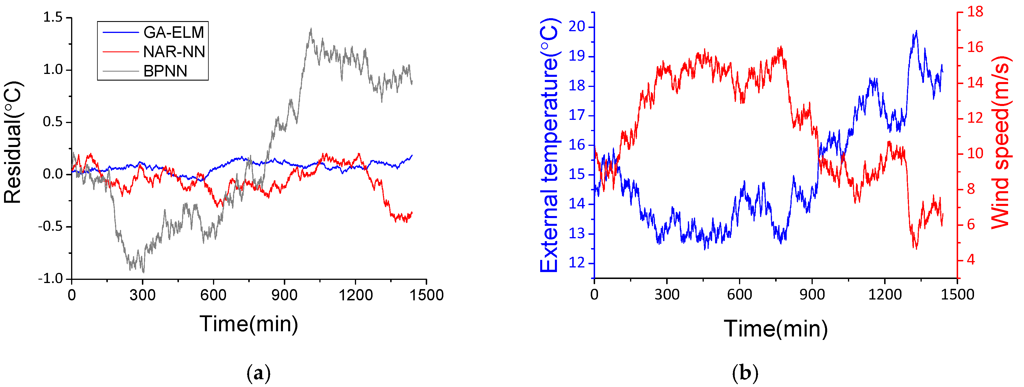
4.2. Model Testing Result

To verify the GA optimization, the original ELM and Back-Propagation Neural Network (BPNN) are used for comparison with GA-ELM. The residuals of GA-ELM, ELM, and BPNN are shown in Figure 7a; the ambient temperature and wind speed of the testing set are shown in Figure 7b.

For the testing set, as shown in Figure 7b, the ambient temperature rises wavily and the wind speed drops rapidly after remaining stable for a period of time. This kind of irregularity may not fit the ELM and BPNN model at local minima. Thus, as shown in Figure 7a, the residual temperature of GA-ELM is smaller than that of ELM and BPNN.

To quantitatively compare the performance of the three algorithms, Mean Square Error (MSE), Mean Absolute Error (MAE), and Mean Absolute Percentage Error (MAPE) are used to analyze the results and calculated as

$$\mathrm{MSE}=\frac{1}{s}{{\displaystyle \sum }}_{k=1}^s{(e_k)}^2$$

(11)

$$\mathrm{MAE}=\frac{1}{s}{\displaystyle \sum }_{k=1}^s\left|e_k\right|$$

(12)

$$\mathrm{MAPE}=\frac{1}{s}{\displaystyle \sum }_{k=1}^s\left|\frac{e_k}{Y_k}\right|$$

(13)

Statistical indicators are shown in

Table 2. Statistical indicators of different intelligent algorithms.

Criteria	GA-ELM	ELM	BPNN
MSE	0.10	0.21	0.58
MAE	0.19	0.59	0.91
MAPE (%)	0.26	0.73	1.84
Time (s)	3.46	3.22	3.15

. In this study, all calculations are performed with the MATLAB R2017b environment on a 64-bit Windows operating system installed on a computer with an Intel Core i7-6700 CPU with 4GHz.

Compared to ELM and BPNN, GA-ELM achieves a smaller MSE, MAE, and MAPE, demonstrating that the GA optimization is effective and the accuracy of the WT model is improved.

5. Case Study

To verify the proposed method, this paper sets up experiments for different ambient conditions and real failure. For an extreme ambient temperature, cases of winter midnight, summer noon, and a cold wave in normal state are presented. For wind speed change, cases of wind speed increase and decrease in normal state are presented. Meanwhile, for failure detection, a main bearing offset case is presented as well.

In these experiments, a comparison method is also applied to analyze the effects of the ambient conditions. The framework of the comparison method is the same as that of the proposed method, as shown in Figure 5. The comparison method uses the same GA-ELM model as the proposed method. The only difference between the proposed method and the comparison method is that the inputs of the comparison method, as with existing methods, do not contain the ambient conditions. To compensate for this, four other parameters (pitch motor 1, 2 and 3 temperature and hub ambient temperature) are added to the inputs of the comparison method. It should be noted that the residual in this paper is the difference in the actual value minus the predicted value. Moreover, for concise description, the proposed method in this paper is referred to as Method I, and the comparison method is referred to as Method II.

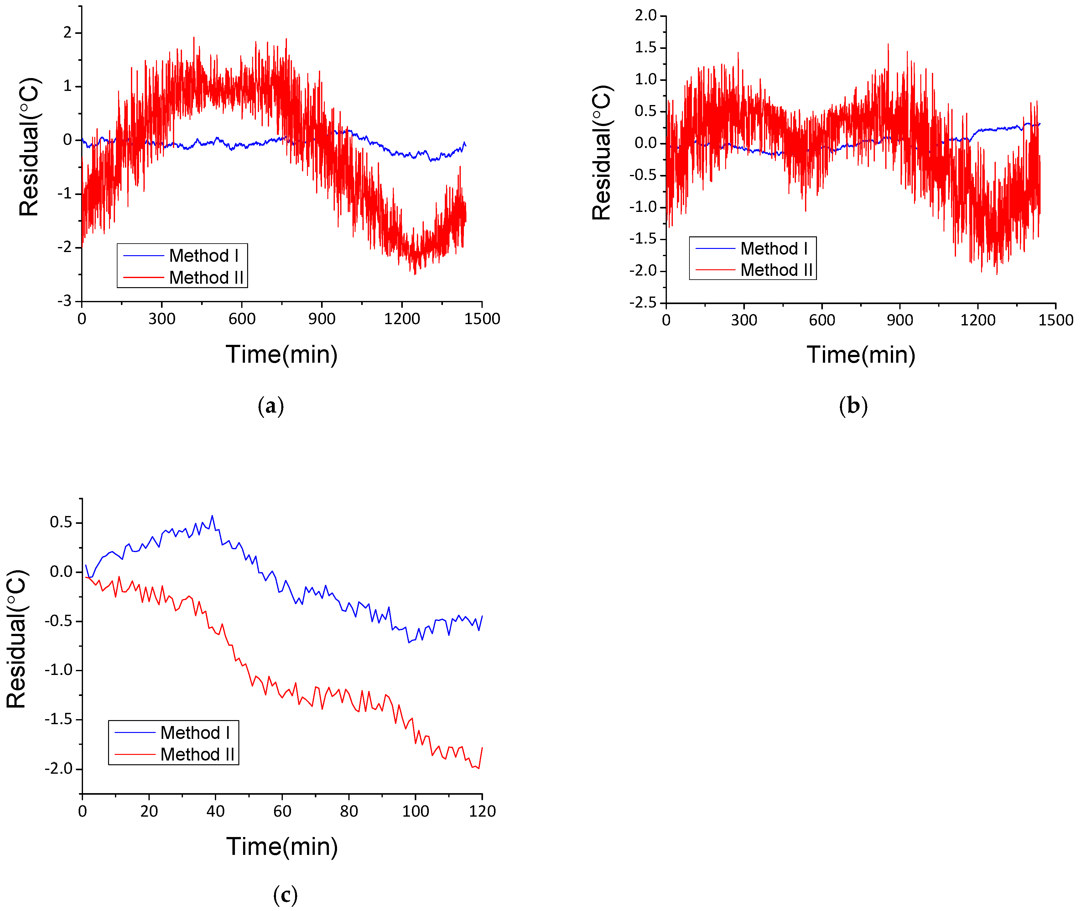
5.1. Ambient Temperature Change in Normal State

For ambient temperature, the data in winter, summer, and the cold wave are shown in

Table 3. Description of datasets under different weather conditions.

Dataset	Start and End Time	Number of Data	Ambient Temperature	Wind Speed
Winter	28 January 00:00–23:59	1440	(−10.58,−0.02) °C	(9.75, 19.38) m/s
Summer	30 July 00:00–23:59	1440	(25.93, 36.59) °C	(4.24, 8.61) m/s
Cold wave	24 Feberary 18:30–20:30	120	(2.84, 16.32) °C	(15.63, 17.85) m/s

. It should be noted that, during these three periods, the WT is in a normal working state.

The residual results are shown in Figure 8, and the statistical indicators are shown in

Table 4. Statistical indicators of Method I and II under a normal working state under different weather conditions.

Criteria	Winter		Summer		Cold Wave
	Method I	Method II	Method I	Method II	Method I	Method II
MSE	0.18	0.91	0.16	0.62	0.18	1.39
MAE	0.14	0.98	0.11	0.73	0.19	1.07
MAPE (%)	0.25	1.79	0.16	1.04	0.30	1.96

.

It can be seen from Figure 8a that the Method I residual results are between −0.45 °C and 0.23 °C, but the Method II residual results are between −2.52 °C and 1.86 °C. Similarly, in Figure 8b, the Method II residual results (between −2.12 °C and 1.67 °C) are much greater than the Method I residual results (between−0.19 °C and 0.28 °C) in summer. Table 4 also shows that Method I achieves smaller statistical indicators than Method II. This proves that, with ambient temperature and ambient temperature change, Method I achieves better performance when facing cyclical and seasonal ambient temperature changes.

Furthermore, comparing Figure 8a,b the effect of ambient temperature in summer is smaller than in winter. A reasonable explanation is that the difference between the main bearing temperature and the ambient temperature is smaller in summer than in winter, since the range of the main bearing temperature in a normal working state is approximately 55–70 °C.

During the cold wave shown in Figure 8c, Method I has some reasonable fluctuations, but Method II shows a downward trend. If the monitoring is based on Method II, the main bearing temperature continues to decline for 2 h, which may lead to false alarms. However, the actual situation is that the WT is under a normal working state. This proves that, although Method II has more temperature parameters as compensation, Method I is more sensitive to the rapid ambient temperature change than Method II.

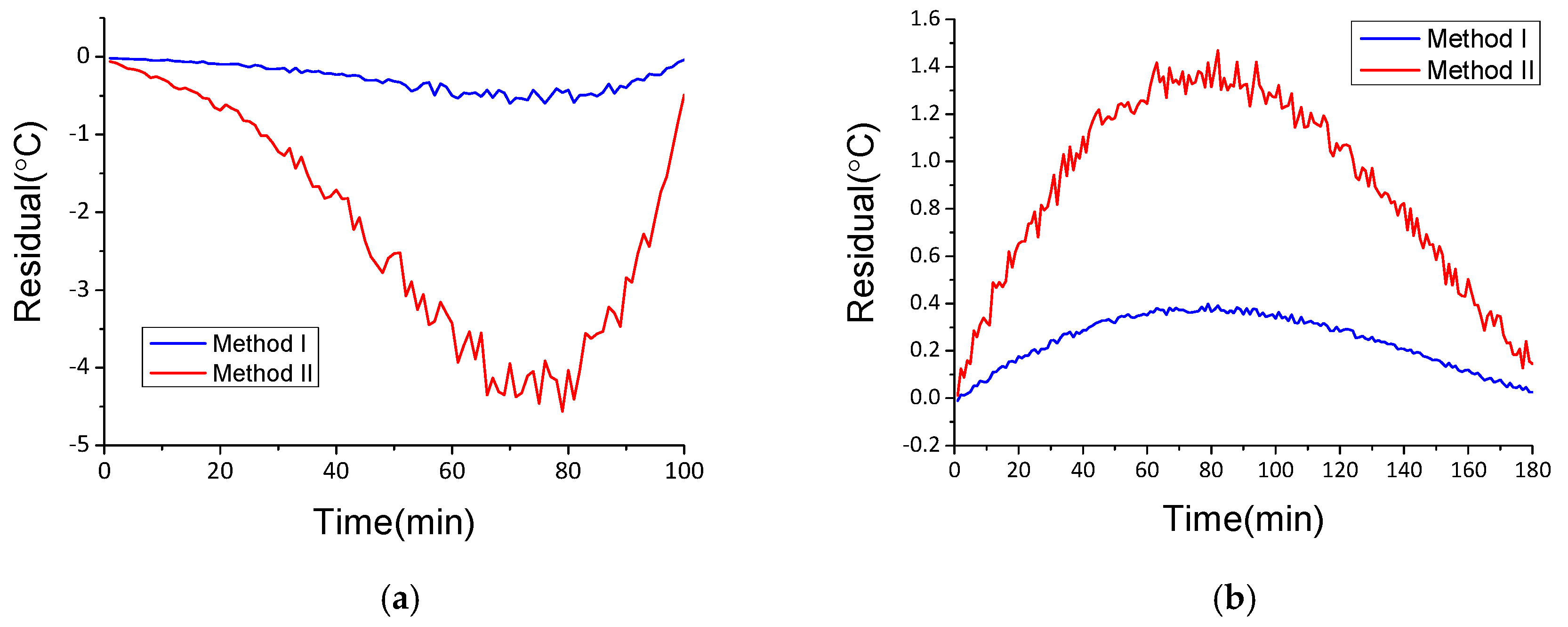
5.2. Wind Speed Change in Normal State

For wind conditions, the datasets of wind speed increase and decrease are shown in

Table 5. Datasets of wind speed increase and decrease.

Dataset	Start and End Time	Number of Data	Ambient Temperature	Wind Speed
Wind speed increase	12 April 09:00–10:39	100	(13.92, 15.01) °C	(4.64, 15.12) m/s
Wind speed decrease	15 April 14:00–16:59	180	(14.45, 15.89) °C	(3.97, 14.83) m/s

. Similarly, in these two periods, the WT is in a normal working state. At the same time, in the event that the ambient temperature would have an influence, the ambient temperature is around 15 °C.

The residual results of Method I and II are shown in Figure 9, and the statistical indicators are shown in

Table 6. Statistical indicators of Method I and II in normal working state during wind speed increase and decrease.

Criteria	Wind Speed Increase		Wind Speed Decrease
	Method I	Method II	Method I	Method II
MSE	0.15	2.85	0.12	0.95
MAE	0.31	2.19	0.26	0.89
MAPE (%)	0.47	3.48	0.38	1.54

.

As shown in Figure 9a, during the wind speed increase, the residual results of Method I and Method II are negative. As mentioned in Section 2, these results are due to the delay between the wind speed change and internal temperature change. Since the wind speed change is used as a model input of Method I, the delay is reduced effectively, and the residuals’ absolute value of Method I is much smaller than that of Method II. The amplitude of Method I is 0.48 °C, and that of Method II is 4.48 °C. The same reasoning can explain Figure 9b: during the wind speed decrease, the residuals’ absolute value of Method I is much smaller than that of Method II (0.39 °C vs. 1.48 °C, respectively). The statistical indicators in Table 6 also prove that Method I achieves better performance than Method II during the wind speed change.

Additionally, both Method I and II achieve better performance during a wind speed decrease than during an increase. These results occur because the speed of wind speed change can directly determine the delay between the wind speed change and internal temperature change. In these two periods, the wind speed increase is faster than the decrease, which means that the delay during the increase is larger than during the decrease. Thus, the absolute values of the residual results during the wind speed increase are generally larger than those during the decrease.

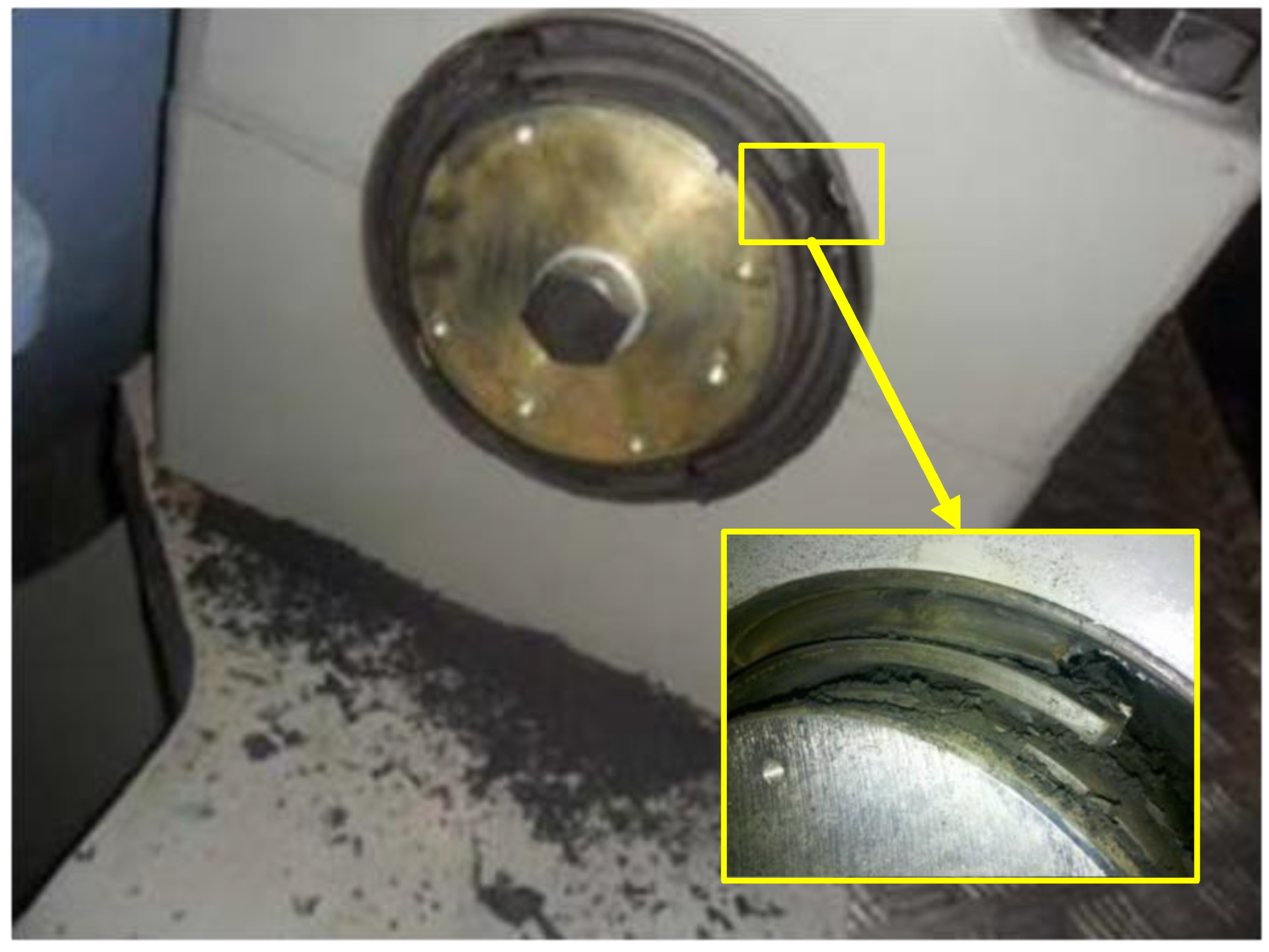
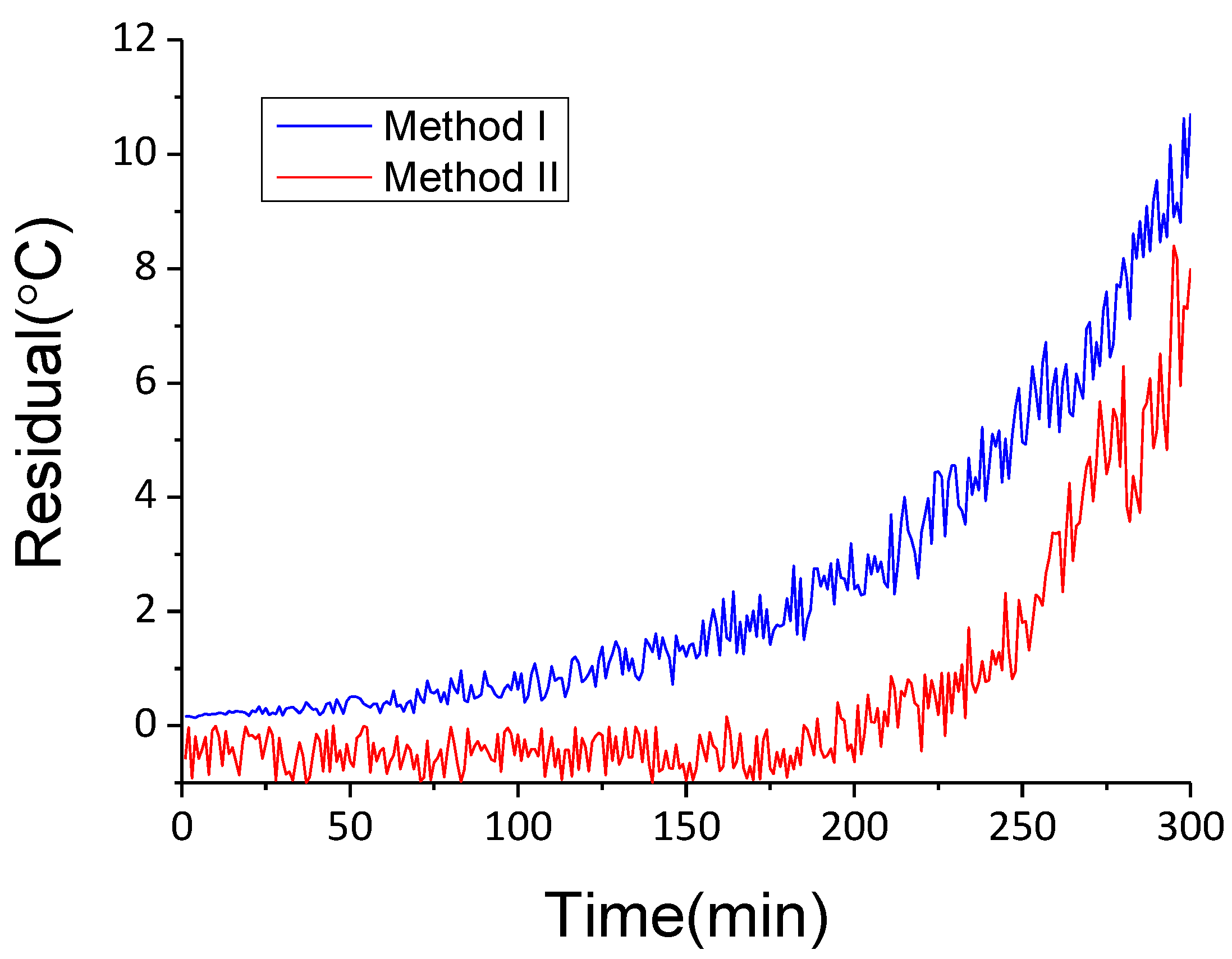
5.3. Main Bearing Failure Detection

To verify the failure detection ability of the proposed method, a serious main bearing offset that occurred in the wind farm, which is shown in Figure 10, is used as a failure case. The dataset of 5 h before the failure happened is shown in

Table 7. Datasets of main bearing offset failure.

Dataset	Start and End Time	Number of Data	Ambient Temperature	Wind Speed
Failure	18 Mar 05:40–10:39	300	(−5.58, 0.02) °C	(3.64, 17.86) m/s

, and the residual results are shown in Figure 11.

The residual results of Method I and Method II both show upward trends, which means that both methods could predict the failure. However, during the 5h period, the ambient temperature continued to drop and the wind speed continued to increase, which caused the residual results of Method II at first to be negative, falling behind Method I. In particular, at 10:16 (time point 276), the wind speed increased rapidly, which caused the residual results of Method II to decrease over a short time. Comparing the two curves, it can be seen that Method II generally falls behind Method I by more than 50 min, reaching approximately90 min at a residual result of 2 °C.

Considering the conclusions of the previous experiments, Method I exhibits stable performance during extreme ambient temperatures and wind speed change, and the residual results of Method I are generally less than 0.5 °C. However, for Method II, due to the change in the ambient conditions, residual results could be more than 1 °C, sometimes reaching 4 °C, under a normal working state. Thus, the safe range of Method I is narrower than that of Method II. If the safe range of Method I is set to ±1 °C and that of Method II is set to ±2 °C, the alarm from Method I would be approximately120 min earlier than in Method II. If the safe range of Method I is set to ±0.5 °C and that of Method II is set to ±4 °C, the alarm of Method I would be more than 180 min earlier than that of Method II. These results demonstrate that Method I, with ambient conditions, can achieve higher monitoring accuracies and earlier failure alarms.

6. Conclusions

WTs are exposed to harsh conditions year-round, and the variability of ambient conditions can affect WT monitoring directly. The main bearing temperature can be different in the same working state but different under ambient temperature and wind speed changes. Conversely, a data-driven model may fall into local minima due to the randomness of the initial coefficients, which can also affect the monitoring accuracy.

To solve these problems, a novel WT monitoring method is proposed. The changes in ambient conditions are used as inputs of the WT model, and the GA-ELM is applied to construct the WT model. Model testing shows that, compared to ELM and BPNN, GA-ELM can avoid local minima and achieve smaller MSE, MAE, and MAPE. With cases in different ambient conditions and real failure, it proves that, compared to the method without considering the change in ambient conditions, the proposed method could reduce false alarms when WT is in a normal working state under extreme ambient conditions, and generate an earlier alarm when a failure is about to occur. This means that the proposed method can reduce operation and maintenance costs, thereby improving the economic efficiency of wind power generation.

It should be noted that this study focuses on ambient temperature and wind speed to describe ambient conditions. However, ambient conditions also include other factors, such as air humidity and air pressure. In future research, these factors should also be considered in order to improve the accuracy of WT monitoring.

References

1. Yaramasu, V.; Wu, B.; Kouro, S. High-power wind energy conversion systems: State-of-the-art and emerging technologies. Proc. IEEE 2015, 103, 740–788. [Google Scholar] [CrossRef]
2. Garrigle, E.M.; Leahy, P.G. Cost Savings from Relaxation of Operational Constraints on a Power System with High Wind Penetration. IEEE Trans. Sustain. Energy 2017, 6, 881–888. [Google Scholar] [CrossRef] [Green Version]
3. Hou, Z.; Zhuang, S.; Lv, X. Monitoring and Analysis of Wind Turbine Condition based on Multivariate Immunity Perception. In Proceedings of the 2019 International Energy and Sustainability Conference (IESC), Farmingdale, NY, USA, 17–18 October 2019; pp. 1–5. [Google Scholar]
4. Xia, G.; Zhou, L.; Minder, J.; Fovell, R.; Jimenez, P. Simulating impacts of real-world wind farms on land surface temperature using the WRF model: Physical mechanisms. Clim. Dyn. 2019, 53, 3. [Google Scholar] [CrossRef]
5. Al-Masri, H.; Ab dullah, A.; AlmehiziaEhsani, M. Accurate Wind Turbine Annual Energy Computation by Advanced Modeling. IEEE Trans. Ind. Appl. 2017, 3, 1. [Google Scholar] [CrossRef]
6. Bakdi, A.; Kouadri, A.; Mekhilef, S. A data-driven algorithm for online detection of component and system faults in modern wind turbines at different operating zones. Renew. Sustain. Energy Rev. 2019, 103, 546–555. [Google Scholar] [CrossRef]
7. Long, H.; Wang, L.; Zhang, Z.; Song, Z.; Xu, J. Data-Driven Wind Turbine Power Generation Performance Monitoring. IEEE Trans. Ind. Electron. 2015, 62, 6627–6635. [Google Scholar] [CrossRef]
8. Kusiak, A.; Zhang, Z. Short-Horizon Prediction of Wind Power: A Data-Driven Approach. Energy Conversion. IEEE Trans. Ind. Electron. 2010, 25, 1112–1122. [Google Scholar]
9. Reder, M.; Yurusen, N.Y.; Melero, J.J. Data-driven learning framework for associating weather conditions and wind turbine failures. Reliab. Eng. Syst. Saf. 2018, 169, 554. [Google Scholar] [CrossRef] [Green Version]
10. Yin, S.; Wang, G.; Karimi, H.R. Data-driven design of robust fault detection system for wind turbines. Mechatronics 2014, 24, 298–306. [Google Scholar] [CrossRef]
11. Yang, W.; Court, R.; Jiang, J. Wind turbine condition monitoring by the approach of SCADA data analysis. Renew. Energy 2013, 53, 365–376. [Google Scholar] [CrossRef]
12. Mazur, D.C.; Entzminger, R.A.; Kay, J.A. Enhancing Traditional Process SCADA and Historians for Industrial & Commercial Power Systems with Energy (Via IEC 61850). IEEE Trans. Ind. 2016, 52, 76–82. [Google Scholar]
13. MDIlicXie, L.; Joo, J.Y. Efficient Coordination of Wind Power and Price-Responsive Demand—Part I: Theoretical Foundations. Power Systems. IEEE Trans. 2011, 26, 1875–1884. [Google Scholar]
14. Velandia-Cardenas, C.; Vidal, Y.; Pozo, F. Wind Turbine Fault Detection Using Highly Imbalanced Real SCADA Data. Energies 2021, 14, 1728. [Google Scholar] [CrossRef]
15. Kusiak, A.; Li, W. Virtual Models for Prediction of Wind Turbine Parameters. IEEE Trans. Energy Convers. 2010, 25, 245–252. [Google Scholar] [CrossRef]
16. Peng, G.; Infield, D. Wind Turbine Tower Vibration Modeling and Monitoring by the Nonlinear State Estimation Technique (NSET). Energies 2012, 5, 5279–5293. [Google Scholar]
17. Wang, Y.; Infield, D.G. Multi-machine Based Wind Turbine Gearbox Condition Monitoring Using Nonlinear State Estimation Technique. EWEA 2014, 2014. [Google Scholar] [CrossRef]
18. Zhao, W.S.; Qu, C.Y.; Zhang, H.B. Direct-Drive Wind Turbine Fault Diagnosis Based on Logistic Regression. In Proceedings of the 15th International Computer Conference on Wavelet Active Media Technology and Information Processing (ICCWAMTIP), Chengdu, China, 14–16 December 2018. [Google Scholar]
19. Wu, F.T.; Wang, C.C.; Liu, J.H.; Chang, C.-M.; Lee, Y.-P. Construction of Wind Turbine Bearing Vibration Monitoring and Performance Assessment System. J. Signal Inf. Process. 2013, 4, 430–438. [Google Scholar] [CrossRef] [Green Version]
20. Wenyi, L.; Zhenfeng, W.; Jiguang, H.; Guangfeng, W. Wind turbine fault diagnosis method based on diagonal spectrum and clustering binary tree SVM. Renew. Energy 2013, 50, 1–6. [Google Scholar] [CrossRef]
21. Santos, P.; Villa, L.; Renones, A.; Bustillo, A. An SVM-Based Solution for Fault Detection in Wind Turbines. Sensors 2015, 15, 5627–5648. [Google Scholar] [CrossRef] [Green Version]
22. Kandukuri, S.T.; Senanayaka, J.; Huynh, K.V.; Robbersmyr, K.G. A Two-Stage Fault Detection and Classification Scheme for Electrical Pitch Drives in Offshore Wind Farms Using Support Vector Machine. IEEE Trans. Ind. Appl. 2019, 55, 5109–5118. [Google Scholar] [CrossRef]
23. Rahimilarki, R.; Gao, Z.; Zhang, A.; Binns, R. Robust neural network fault estimation approach for nonlinear dynamic systems with applications to wind turbine systems. IEEE Trans. Ind. Inform. 2019, 15, 6302–6312. [Google Scholar] [CrossRef]
24. Bangalore, P.; Tjernberg, L.B. An Artificial Neural Network Approach for Early Fault Detection of Gearbox Bearings. IEEE Trans. Smart Grid 2017, 6, 980–987. [Google Scholar] [CrossRef]
25. Qu, F.; Liu, J.; Liu, X.; Jiang, L. A Multi-fault Detection Method with Improved Triplet Loss Based on Hard Sample Mining. IEEE Trans. Sustain. Energy 2020, 12, 127–137. [Google Scholar] [CrossRef]
26. Zhang, J.; Sun, H.; Sun, Z.; Dong, W.; Dong, Y. Fault Diagnosis of Wind Turbine Power Converter Considering Wavelet Transform, Feature Analysis, Judgment and BP Neural Network. IEEE Access 2019, 7, 179799–179809. [Google Scholar] [CrossRef]
27. Kusiak, A.; Zhang, Z.; Li, M. Optimization of Wind Turbine Performance with Data-Driven Models. IEEE Trans. Sustain. Energy 2010, 1, 66–76. [Google Scholar] [CrossRef]
28. Ak, R.; Fink, O.; Zio, E. Two Machine Learning Approaches for Short-Term Wind Speed Time-Series Prediction. IEEE Trans. Neural Netw. Learn. Syst. 2016, 27, 1734–1747. [Google Scholar] [CrossRef]
29. Li, S.; Wang, P.; Goel, L. Short-term load forecasting by wavelet transform and evolutionary extreme learning machine. Electr. Power Syst. Res. 2015, 122, 96–103. [Google Scholar] [CrossRef]
30. Wan, C.; Xu, Z.; Pinson, P. Probabilistic forecasting of wind power generation using extreme learning machines. IEEE Trans. Power Syst. 2014, 29, 1033–1044. [Google Scholar] [CrossRef] [Green Version]
31. Wan, C.; Xu, Z.; Wang, Y. A hybrid approach for probabilistic forecasting of electricity prices. IEEE Trans. Smart Grid 2014, 5, 463–470. [Google Scholar] [CrossRef]
32. Wan, C.; Zhao, X.; Pierre, P. Optimal prediction intervals of wind power generation. IEEE Trans. Power Syst. 2014, 29, 1166–1174. [Google Scholar] [CrossRef] [Green Version]
33. Liu, S.; Hou, Z.; Yin, C. Data-Driven Modeling for UGI Gasification Processes via an Enhanced Genetic BP Neural Network with Link Switches. IEEE Trans. Neural Netw. Learn. Syst. 2015, 27, 2718–2729. [Google Scholar] [CrossRef] [PubMed]
34. Shen, X.; Zheng, Y.; Zhang, R. A Hybrid Forecasting Model for the Velocity of Hybrid Robotic Fish Based on Back-Propagation Neural Network with Genetic Algorithm Optimization. IEEE Access 2020, 8, 111731–111741. [Google Scholar] [CrossRef]
35. Kaleeswaran, V.; Dhamodharavadhani, S.; Rathipriya, R. A Comparative Study of Activation Functions and Training Algorithm of NAR Neural Network for Crop Prediction. In Proceedings of the 2020 4th International Conference on Electronics, Communication and Aerospace Technology (ICECA), Coimbatore, India, 5–7 November 2020. [Google Scholar]
36. Villanueva, D.; AFeijó, A. Normal-Based Model for True Power Curves of Wind Turbines. IEEE Trans. Sustain. Energy 2016, 7, 1005–1011. [Google Scholar] [CrossRef]
37. Xie, K.; Jiang, Z.; Li, W. Effect of Wind Speed on Wind Turbine Power Converter Reliability. IEEE Trans. Energy Convers. Ec. 2012, 27, 96–104. [Google Scholar] [CrossRef]
Figure 1. WT in normal state: (a) active power–wind speed; (b) main bearing temperature–wind speed.
Energies 14 07529 g001
Figure 2. Main bearing temperature during wind speed increase and decrease.
Energies 14 07529 g002
Figure 3. Main bearing temperature within different ambient temperatures.
Energies 14 07529 g003
Figure 4. Main bearing temperature during cold wave.
Energies 14 07529 g004
Figure 5. Framework of the proposed method.
Energies 14 07529 g005
Figure 6. Topology of Extreme Learning Machine (ELM).
Energies 14 07529 g006
Figure 7. (a) Model testing results of different intelligent algorithms; (b)ambient conditions of testing set.
Energies 14 07529 g007
Figure 8. Residual results of Method I and II under a normal working state under different weather conditions: (a) winter; (b) summer; (c) cold wave.
Energies 14 07529 g008
Figure 9. Residual results of Method I and II in normal working state within wind conditions: (a) wind speed increase; (b) wind speed decrease.
Energies 14 07529 g009
Figure 10. Main bearing offset failure.
Energies 14 07529 g010
Figure 11. Residual results of Method I and II in main bearing offset failure.
Energies 14 07529 g011