Application of Empirical Mode Decomposition and Extreme Learning Machine Algorithms on Prediction of the Surface Vibration Signal

Abstract

Accurately predicting surface vibration signals of diesel engines is the key to evaluating the operation quality of diesel engines. Based on an improved empirical mode decomposition and extreme learning machine algorithm, the characteristics of diesel engine surface vibration signal were detected, predicted, and analyzed. First, the surface vibration signal was decomposed into a series of signal components by an improved empirical mode decomposition algorithm. Then, the extreme learning machine algorithm was applied to each signal component to obtain the predicted value of the corresponding signal component and determine the characteristics of the ground vibration signal. Compared with the empirical mode decomposition–extremum learning machine algorithm and the extremum learning machine algorithm, the results show that the improved empirical mode decomposition–extremum learning machine algorithm is feasible and effective.

1. Introduction

With the progress of science and technology, as the power source of large rotating machinery, diesel engines need continuous innovation. Because it is a large workload to evaluate the performance of a diesel engine directly through the structural parameters of the engine, researchers have always analyzed the performance of diesel engines by studying vibration signals [1,2]. Owing to the non-stationary and nonlinear characteristics of the vibration signal of a diesel engine in rotating machinery [3,4], it is difficult to predict it effectively. Therefore, methods to predict the vibration signal of the diesel engine effectively have received extensive attention.

Traditional vibration analysis methods mainly include time–domain analysis, such as extracting the mean amplitude, kurtosis, and other indicators of the signal, but it is difficult to reveal the frequency composition of the signal, the size of each frequency component, and other internal information [5]. Forms of frequency domain analysis include Fourier transform (FT) [6,7]; time–frequency analysis, such as short-time Fourier transform (STFT) [8], wavelet transform (WT) [9,10], etc. Compared with other methods, empirical mode decomposition (EMD) [11,12] does not need signal preprocessing in advance; it can decompose signals adaptively layer by layer. The results of this decomposition are finite intrinsic mode functions (IMFs), and it is unnecessary to obtain the prior knowledge of signals during this decomposition process. However, the EMD method is an empirical method, which lacks strong and strict theoretical support and still has many mathematical problems to be solved [13]. The EMD method itself is still not perfect; there are still some problems, such as mode mixing [14,15], endpoint effect [16,17], determination of termination criteria [18,19], and EMD can only be used for the analysis of one-dimensional real signals. Tang et al. [20] proposed a method to eliminate mode aliasing in EMD based on improved blind source separation technology. V. G. Kurbatskii et al. [21] proposed a two-stage adaptive approach for time series forecasting. The efficiency of the developed approach was displayed in a real-time series in the electric power problem of forecasting the sharply variable implementations of active power flows. Hu et al. [22] proposed a back-projection method to deal with mode aliasing in EMD based on the assumption that every inherent mode function should be locally orthogonal. Hu N Q et al. [23] used EMD and a deep convolutional neural network for fault diagnosis in a planetary gearbox. V. G. Kurbatskii et al. [24] proposed a modification of the adaptive approach to time series forecasting. A hybrid genetic algorithm training for an artificial neural network and a regression model based on a support-vector machine were established to verify the effectiveness of the method. Xu K et al. [25] proposed a rolling bearing fault diagnosis method based on EMD and a support-vector machine. Tim Leung et al. [26] proposed the method of complementary ensemble empirical mode decomposition (CEEMD) and the Hilbert–Huang transform (HHT) for analyzing nonstationary financial time series. Using a series of examples of empirical financial data, they verified how HHT features enhanced machine learning models in terms of predictive performance. Manohar Mishra et al. [27] studied the detection of power system voltage sag causes (VSCs), and the interference-balanced voltage signals extracted from relay points were extracted by the signal processing algorithm. Then, VSCs were identified using the input to an extreme learning machine (ELM). To verify the accuracy of the proposed method, ELM performance was compared with manual neural network (ANN), K-nearest Neighbor (KNN), and support-vector machine (SVM) classifiers to verify its validity.

In this paper, a combined algorithm based on improved EMD and ELM [28,29] was proposed to predict surface vibration signals for the first time, taking advantage of EMD’s good processing of densely distributed signals and ELM’s ability to accurately describe transient parameter characteristics of non-stationary signals. The original signal is processed by the EMD algorithm to reduce the complexity of the time series. The improved EMD algorithm performs midpoint fitting for the interval to better solve the error caused by interpolation. Therefore, the improved EMD algorithm overcomes the phenomenon of EMD mode aliasing and is robust to noise. Finally, compared with the EMD-ELM combined algorithm, the effectiveness of the IEMD-ELM combined algorithm is verified. All experiments were performed in a diesel engine laboratory.

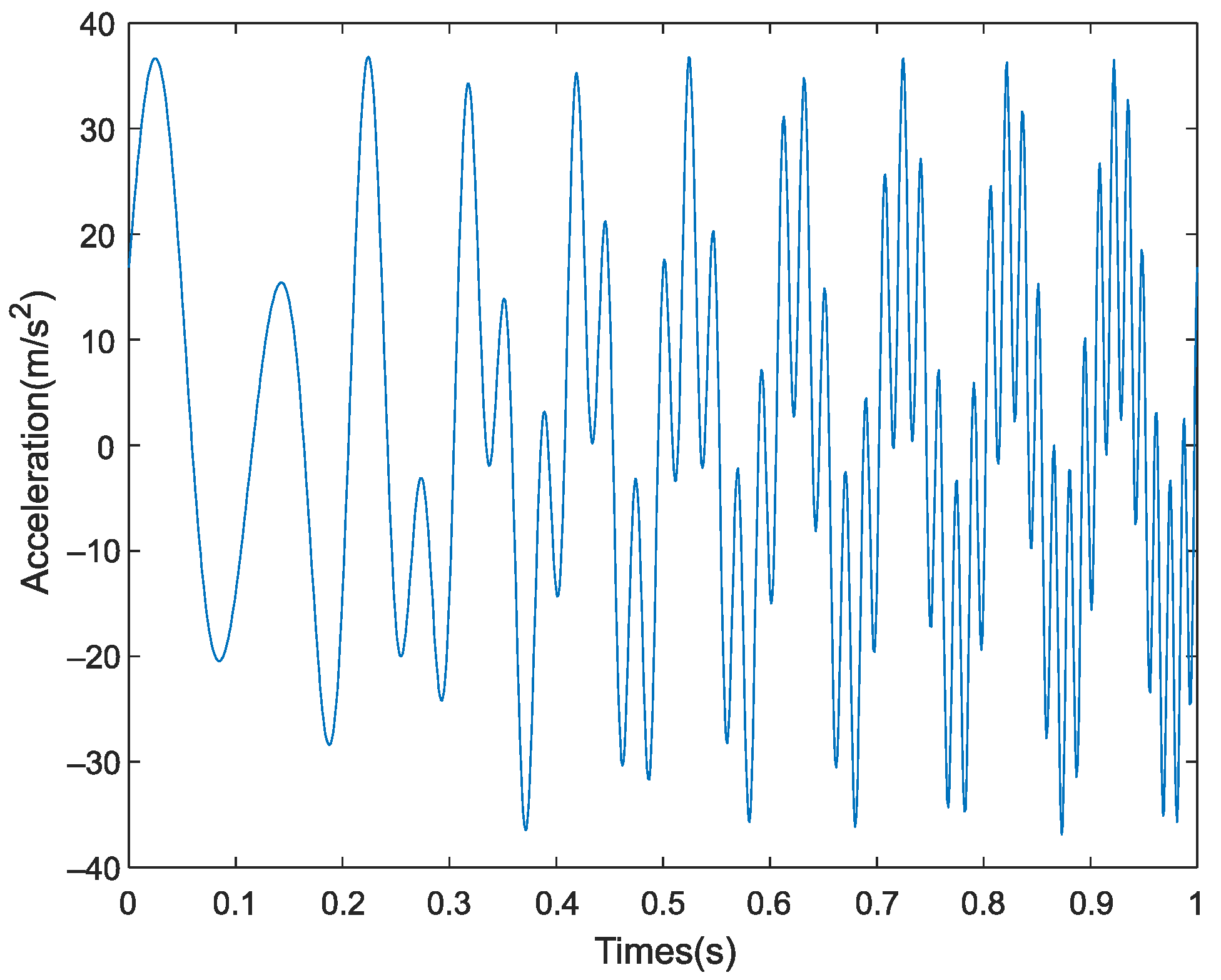
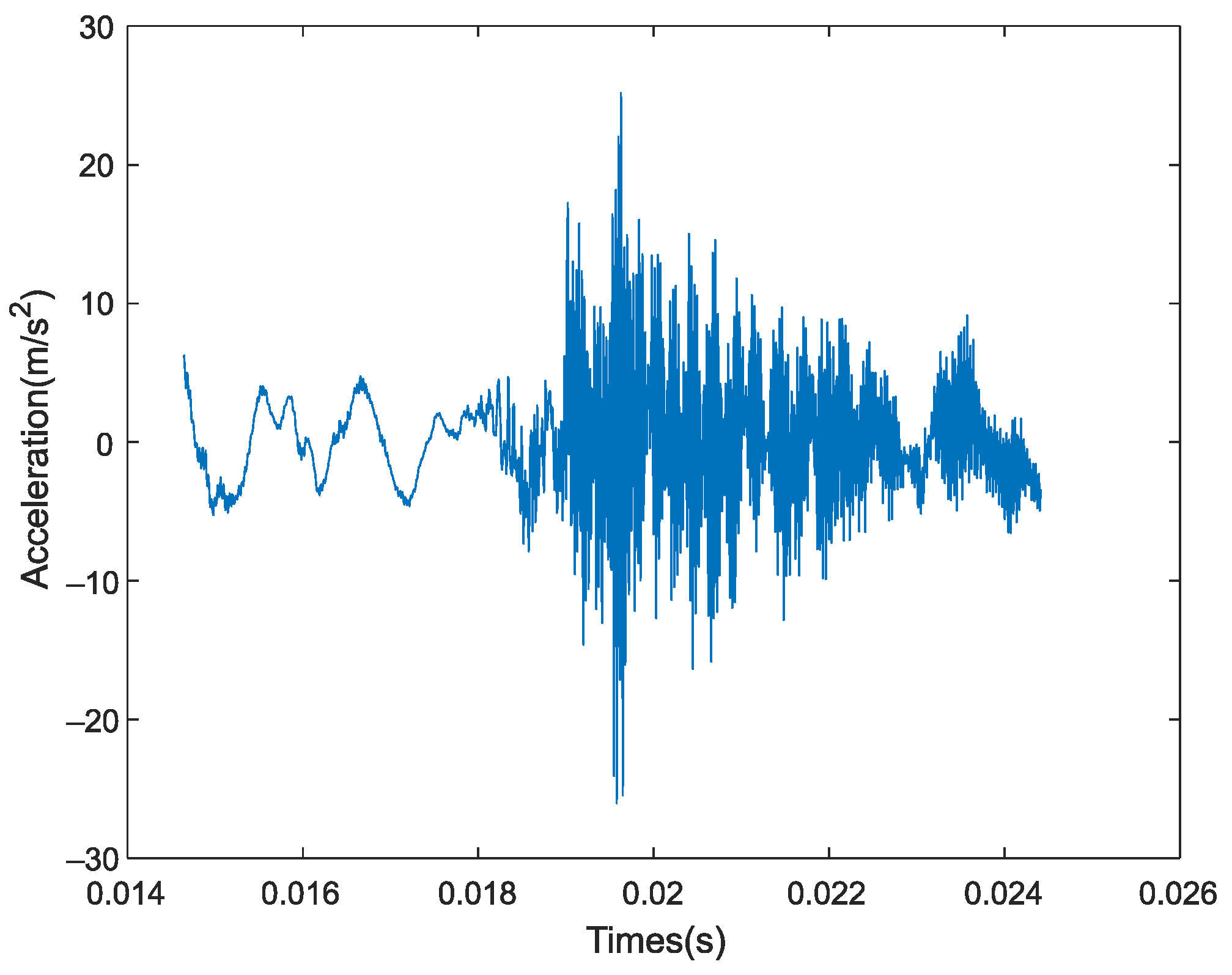
2. Definition of Surface Vibration Signal

In this section, the compositions of surface vibration signals are defined and analyzed.

The surface vibration signal includes two main parts and can be defined as follows:

$$V(t)={\displaystyle {\sum }_{i=1}^n{X}_i(t)}+N(t)$$

(1)

where ${\displaystyle {\sum }_{i=1}^n{X}_i(t)}$ is the main surface vibration signal component, $N(t)$ represents the noise interference, and $n$ is the number of the main component.

The main component of the surface vibration signal can be further defined as follows:

$${\displaystyle {\sum }_{i=1}^n{X}_i(t)}=X_1\cos ({\omega }_{1}t+{\varphi }_1)+X_2\cos ({\omega }_{2}t+{\varphi }_2)+\cdots +X_n\cos ({\omega }_{n}t+{\varphi }_n)$$

(2)

where ${\varphi }_i$ represents the initial phase angle of the ith major component.

3. The Proposed Prediction Algorithms of Surface Vibration Signal Based on EMD-ELM

In this section, a decomposition prediction algorithm of surface vibration signal based on EMD and ELM is proposed. First, the principle of the EMD algorithm is analyzed in detail, then the undershoot interval of EMD is observed and determined. An improved EMD algorithm is used to decompose the complex surface vibration signals into K-order modes, that is, IMFs. Finally, the predicted values of each mode are obtained by the ELM algorithm.

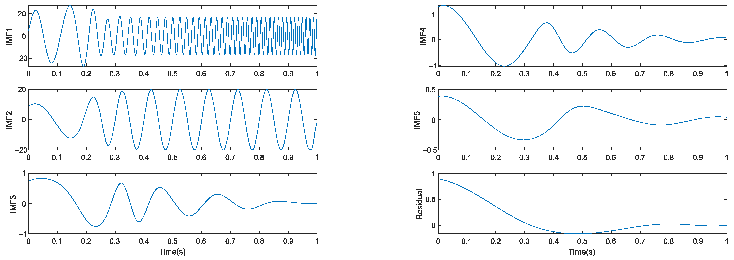
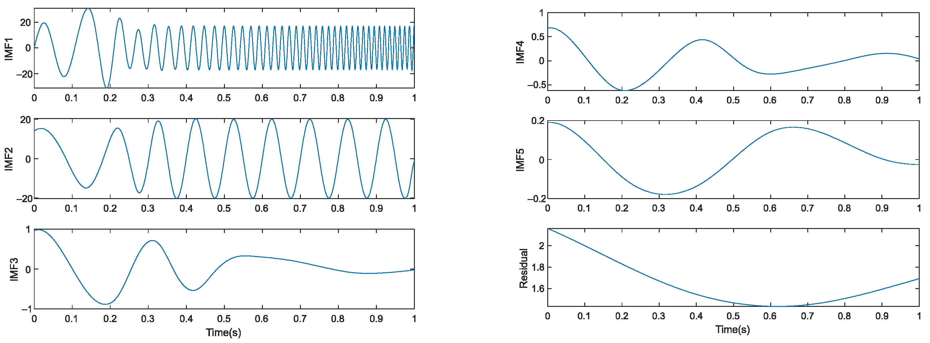
3.1. Empirical Mode Decomposition

In general, the EMD algorithm is an adaptive, quasi-orthogonal method. The EMD algorithm takes all local extreme points of the original signal $V(t)$ as interpolation points; using a cubic spline method to construct the enveloping line, the upper and lower enveloping lines are obtained, and then the average enveloping line $m(t)$ is obtained.

$$m(t)=\frac{f_{\max }(t)+f_{\min }(t)}{2}$$

(3)

where $f_{\max }(t)$ represents the upper enveloping line and $f_{\min }(t)$ represents the lower enveloping line.

Considering $h_1(t)$ as the result of = $V(t)$ minus $m(t)$ means that:

$$h_1(t)=V(t)-m(t)$$

(4)

If $h_1(t)$ satisfies the IMF condition, then the decomposition stops. When $h_1(t)$ does not satisfy the IMF condition, consider $h_1(t)$ as the new original signal as follows, and repeat the above steps until $h_1(t)$ satisfies the IMF condition.

A termination criterion needs to be set. In general, the termination criterion is set to the standard deviation SD values of $h_{1k}(t)$ and $h_{1\left(k-1\right)}(t)$, i.e.,

$$SD={\displaystyle \sum _{t=0}^T\frac{{\left(h_{1k}(t)-h_{1(k-1)}(t)\right)}^2}{h_{1k}^2(t)}}$$

(5)

The orthogonal index (IO) is used to determine the degree of decomposition, which is defined as:

$$IO={\displaystyle \sum _t\frac{{\displaystyle \sum _{i=1}^K{\displaystyle \sum _{j=1}^K{h}_i}}(t)h_j(t)}{V^2(t)}},i\ne j$$

(6)

IO denotes the degree of orthogonality between all modes.

The flow chart for the EMD algorithm is shown in Figure 1.

Figure 1. Flowchart of the empirical mode decomposition (EMD) algorithm.

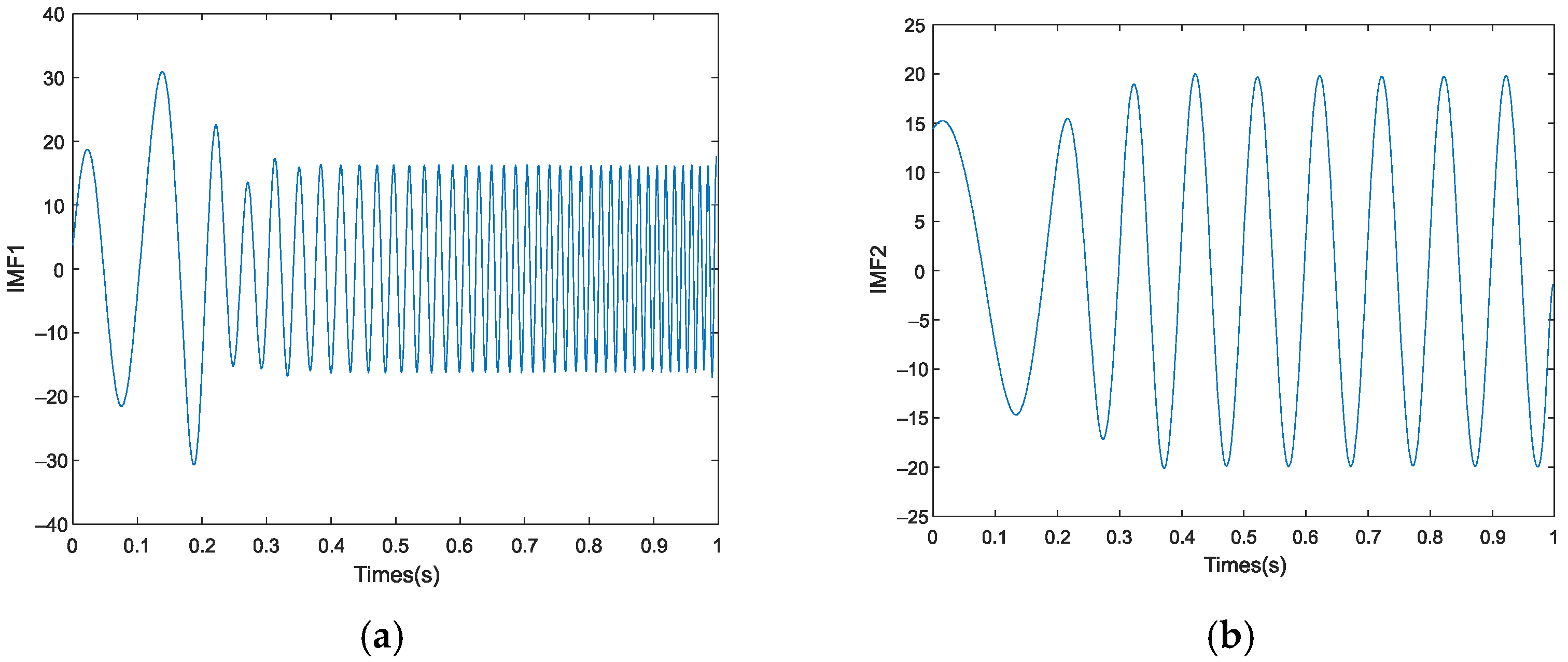
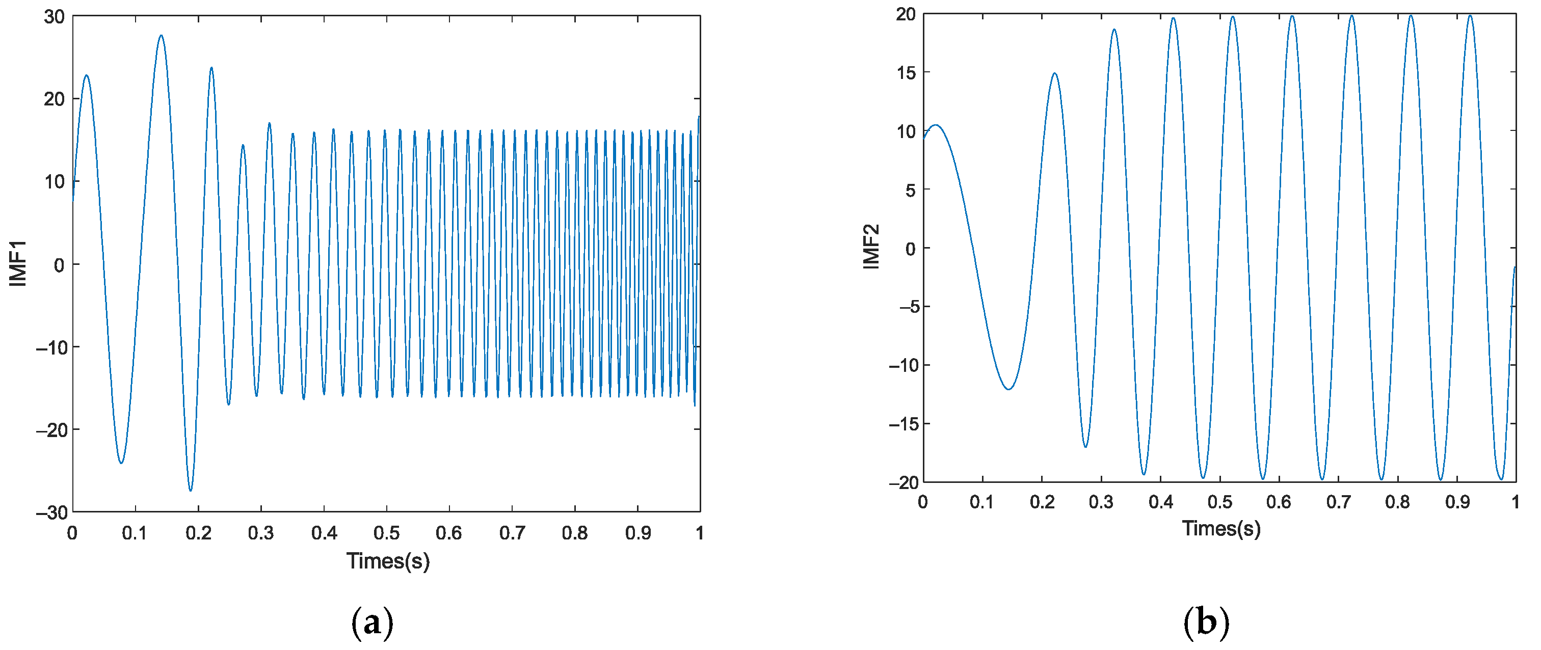
3.2. Improved Empirical Mode Decomposition

This paper presents an improved envelope fitting method to solve the problems of the EMD algorithm. First, find out the local extreme point of the signal, and then find out the midpoint of every two adjacent extreme points:

$$\begin{array}{l}\left(t_{i\max m},y_{i\max m}\right)=\left(\frac{t_{i\max }+t_{i+1\max }}{2},\frac{y_{i\max }+y_{i+1\max }}{2}\right),i=1,2,,,n_{\max }-1\\ \left(t_{i\min m},y_{i\min m}\right)=\left(\frac{t_{i\min }+t_{i+1\min }}{2},\frac{y_{i\min }+y_{i+1\min }}{2}\right),i=1,2,,,n_{\min }-1\end{array}$$

(7)

where $n_{\max }$ and $n_{\min }$ are the number of local maximum and local minimum points of signals, respectively, the midpoint of the extreme point and the original extreme point are taken together as the interpolation nodes, and the second derivative $u^{″}(t)$ at these nodes is first obtained. If the second derivative is not known, it is directly regarded as the natural boundary condition; that is, the value of the second derivative at the two endpoints is zero, and then the initial envelope $u_0(t)$ after fitting is obtained using the cubic spline method.

Determine the area where the undershoot and the data value in the signal are greater than the fitting value of the corresponding point of the envelope. There must be $u_0(t)\ge V(t)$ covering over the entire interval $V(t)$. Therefore, if there is a region with undershoot and the data value in the signal is greater than the function value of the corresponding point of the envelope, the set of that region can be expressed as:

$$\{(t_{a_i,}{t}_{b_i})|V_1(t_{a_i})=V_1(t_{b_i})=0,x_1(t)>0,t\in (t_{a_i},t_{b_i}),i\in N\}$$

(8)

where $V_1(t)=V(t)-u_0(t)$ and $N$ is the number of intervals in which undershoot exists.

Consider the non-negative local maximum of $x_1(t)$ and divide it into two groups:

$$\begin{array}{l}O=\{o_i(t_{o_o},x_1(t_o)),x_1(t_o)=0,i=1,2,\dots \}\\ N=\{N_j(t_{n_j},x_1(t_{n_j})),x_1(t_{n_j}),x_1(t_{n_j})>0,j=1,2,\dots \}\end{array}$$

(9)

Under ideal conditions, $O$ is still the maximum of $V(t)$ and $u_0(t)$ intersects at $O$.

A new envelope, $u_1(t)$ of $V(t)$, is obtained by fitting the horizontal axis of the coordinate axis with points in $O$ and $N$ by cubic spline interpolation. The improved EMD algorithm step is as follows.

Considering $u_1(t)$ as the result of $V(t)$ minus $u_0(t)$ means that:

$$u_1(t)=V(t)-u_0(t)$$

(10)

If $u_1(t)$ satisfies the IMF condition, then the decomposition stops. When $u_1(t)$ does not satisfy the IMF condition, consider $u_1(t)$ as the new original signal as follows, and repeat the above steps until $u_1(t)$ satisfies the IMF condition.

The termination criterion is still set by the standard deviation (SD) values, as in Equation (5).

The flow chart for the improved EMD algorithm is shown in Figure 2.

Figure 2. Flowchart of the improved empirical mode decomposition (IEMD) algorithm.

3.3. Extreme Learning Machine

An extreme learning machine (ELM) is a single hidden layer feedforward neural network learning algorithm. Compared with the traditional neural network, the parameters of its hidden layer neurons are randomly generated. During the training, no recursive adjustment is made and a unique optimal solution is obtained.

The network structure is shown in Figure 3.

Figure 3. The network structure.

This method has the advantages of fast learning speed, high accuracy, simple parameter adjustment, and good generalization ability, and it has been widely used in power load forecasting, power grid reliability assessment, and other fields [30,31,32].

For any N different sample $(x_i,y_i)$, where $x_i={[x_{i1},x_{i2},\cdots ,x_{in}]}^{\mathrm{T}}\in R^n$, $y_i={[y_{i1},y_{i2},\cdots ,y_{in}]}^{\mathrm{T}}\in R^k$, the output expression of a feedforward neural network with l hidden layer nodes and excitation region $G(x)$ is as follows:

$$y_i=f(x_i)={\displaystyle \sum _{j=1}^l{\beta }_{i}G(w_j●x_i+b_j)},w_j\in R^n,{\beta }_j\in R^k$$

(11)

where $i=1,2,\cdots ,N$, $j=1,2,\cdots ,l$,$w_j={[w_{i1},w_{i2},\cdots ,w_{in}]}^{\mathrm{T}}$ is the input weight connecting the input layer to the jth hidden layer node; ${\beta }_j={[{\beta }_{j1},{\beta }_{j2},\cdots ,{\beta }_{jk}]}^{\mathrm{T}}$ is the output weight connecting the jth hidden layer node to the output node to the deviation value of the jth hidden layer node; $w_j\cdot x_i$ is the inner product of $w_j$ and $x_i$; and the excitation function $G(x)$ can be selected as “Sigmoid”, “Tansig”, “Sine”, or “RBF”, etc.

By converting Equation (9) into matrix form, it can be obtained that:

$$Y=H\beta$$

(12)

where $H$ is the output matrix of the hidden layer of the network.

In the ELM algorithm, the input weight and the hidden layer can be given randomly and there is no need for adjustment during the training process. The hidden layer matrix $H$ is a definite matrix before the training. The training of the feedforward neural network is actually transformed into a problem of solving the least square solution $\widehat{\beta }$ of the output weight matrix. The output weight matrix $\beta$ can be expressed as:

$$\widehat{\beta }=H^{+}Y$$

(13)

where $H^{+}$ is the generalized inverse matrix of the matrix $H$.

4. The Simulation Results

In this section, some cases are implemented to elaborate the proposed prediction algorithm based on IEMD-ELM, where both the noise-free and noisy conditions are considered. The sampling frequency is 1 KHz. Additionally, the simulation comparison between IEMD-ELM and EMD-ELM algorithms is conducted in this section.

4.1. Surface Vibration Signal without Noise

Supposing the surface vibration signal as follows:

$$x(t)=20\sin (2\pi \cdot 2t)+17\cos (2\pi \cdot 40t^2)$$

(14)

the amplitude of signal is illustrated in Figure 4.

Figure 4. The signal without noise.

Figure 4 shows the amplitude distribution of the simulation signal without noise.

IEMD and EMD algorithms are used to decompose the input signal. Figure 5 and Figure 6 show the corresponding decomposition patterns.

Figure 5. EMD decomposition.

Figure 6. IEMD decomposition.

As shown in Figure 5 and Figure 6, the signal is decomposed by two different modes and six modal components are obtained.

Presented in Table 1 and Table 2 are the correlation coefficients between IMFs and input signals decomposed by the EMD algorithm and the IEMD algorithm. As defined by the correlation coefficients, the IEMD algorithm has a better decomposition effect than the EMD algorithm.

Table 1. Coefficients under EMD decomposition.

Mode	IMF1	IMF2	IMF3	IMF4	IMF5
Coefficient	0.70	0.68	0.14	0.13	0.09

Table 2. Coefficients under IEMD decomposition.

Mode	IMF1	IMF2	IMF3	IMF4	IMF5
Coefficient	0.73	0.69	0.16	0.13	0.11

Generally, the empirical threshold is set to 0.4. As seen in Table 1, the correlation coefficients of IMF1 and IMF2 obtained after EMD are greater than the empirical threshold. Thus, the next step is predicting IMF1 and IMF2. The prediction of IMF1 and IMF2 is shown in Figure 7.

Figure 7. Performance of prediction under the EMD: (a) IMF1; (b) IMF2.

Figure 7 shows the prediction results of IMF1 and IMF2, and the reconstruction and reduction method based on the prediction results used to obtain the figure is shown in Figure 8.

Figure 8. Reconstruction result after EMD decomposition.

Figure 8 shows the reconstruction result after the EMD and ELM algorithms. The graph trend of the true value and prediction value is consistent, but there is a certain deviation between the prediction result and the true value in the low frequency band.

As seen in Table 2, the correlation coefficients of IMF1 and IMF2 obtained after IEMD are greater than the empirical threshold. The prediction of IMF1 and IMF2 is shown in Figure 9.

Figure 9. Performance of prediction under the IEMD: (a) IMF1; (b) IMF2.

Figure 9 shows the prediction results of IMF1 and IMF2, and the reconstruction and reduction method based on the prediction results used to obtain the figure is shown in Figure 10.

Figure 10. Reconstruction results after IEMD decomposition.

Figure 10 shows the reconstruction result after the IEMD and ELM algorithms. The graph trend of the true value and prediction value is consistent, but the offset between the predicted result and the true value in the low frequency band is smaller than for EMD-ELM.

4.2. Surface Vibration Signal with Noise

To verify the noise robustness of the IEMD algorithm, the simulation signal with noise is given as (13), and the amplitude of signal is illustrated in Figure 11.

$$x(t)=20\sin (2\pi \cdot 2t)+17\cos (2\pi \cdot 40t^2)+randn$$

(15)

where “randn” represents the noise interference.

Figure 11. The signal with noise.

The IEMD and EMD algorithms are used to decompose the input signal. Figure 12 and Figure 13 show the corresponding decomposition patterns.

Figure 12. EMD decomposition.

Figure 13. IEMD decomposition.

Presented in Table 3 and Table 4 are the correlation coefficients between IMFs and input signals decomposed by the EMD algorithm and the IEMD algorithm. As defined by the correlation coefficient, the IEMD algorithm has a better decomposition effect than the EMD algorithm.

Table 3. Coefficients under EMD decomposition.

Mode	IMF1	IMF2	IMF3	IMF4	IMF5
Coefficient	0.70	0.69	0.14	0.13	0.09

Table 4. Coefficients under IEMD decomposition.

Mode	IMF1	IMF2	IMF3	IMF4	IMF5
Coefficient	0.73	0.69	0.16	0.14	0.11

As seen in Table 3, the correlation coefficients of IMF1 and IMF2 obtained after EMD are greater than the empirical threshold. The prediction of IMF1 and IMF2 is shown in Figure 14.

Figure 14. Performance of prediction under the EMD: (a) IMF1; (b) IMF2.

Figure 14 shows the prediction results of IMF1 and IMF2, and the reconstruction and reduction method based on the prediction results used to obtain the figure is shown in Figure 15.

Figure 15. Reconstruction result after EMD decomposition.

Figure 15 shows the reconstruction result after the EMD and ELM algorithms. The graph trend of the true value and prediction value is consistent, but there is a certain deviation between the prediction result and the true value in the low frequency band.

As seen in Table 4, the correlation coefficient of IMF1 and IMF2 obtained after IEMD is greater than the empirical threshold. The prediction of IMF1 and IMF2 is shown in Figure 16.

Figure 16. Performance of prediction under the EMD: (a) IMF1; (b) IMF2.

Figure 16 shows the prediction results of IMF1 and IMF2, and the reconstruction and reduction method based on the prediction results used to obtain the figure is shown in Figure 17.

Figure 17. Reconstruction result after IEMD decomposition.

Figure 17 shows the reconstruction result after the IEMD and ELM algorithms. The graph trend of the true value and prediction value is consistent, but the offset between the predicted result and the true value in the low frequency band is smaller than EMD-ELM.

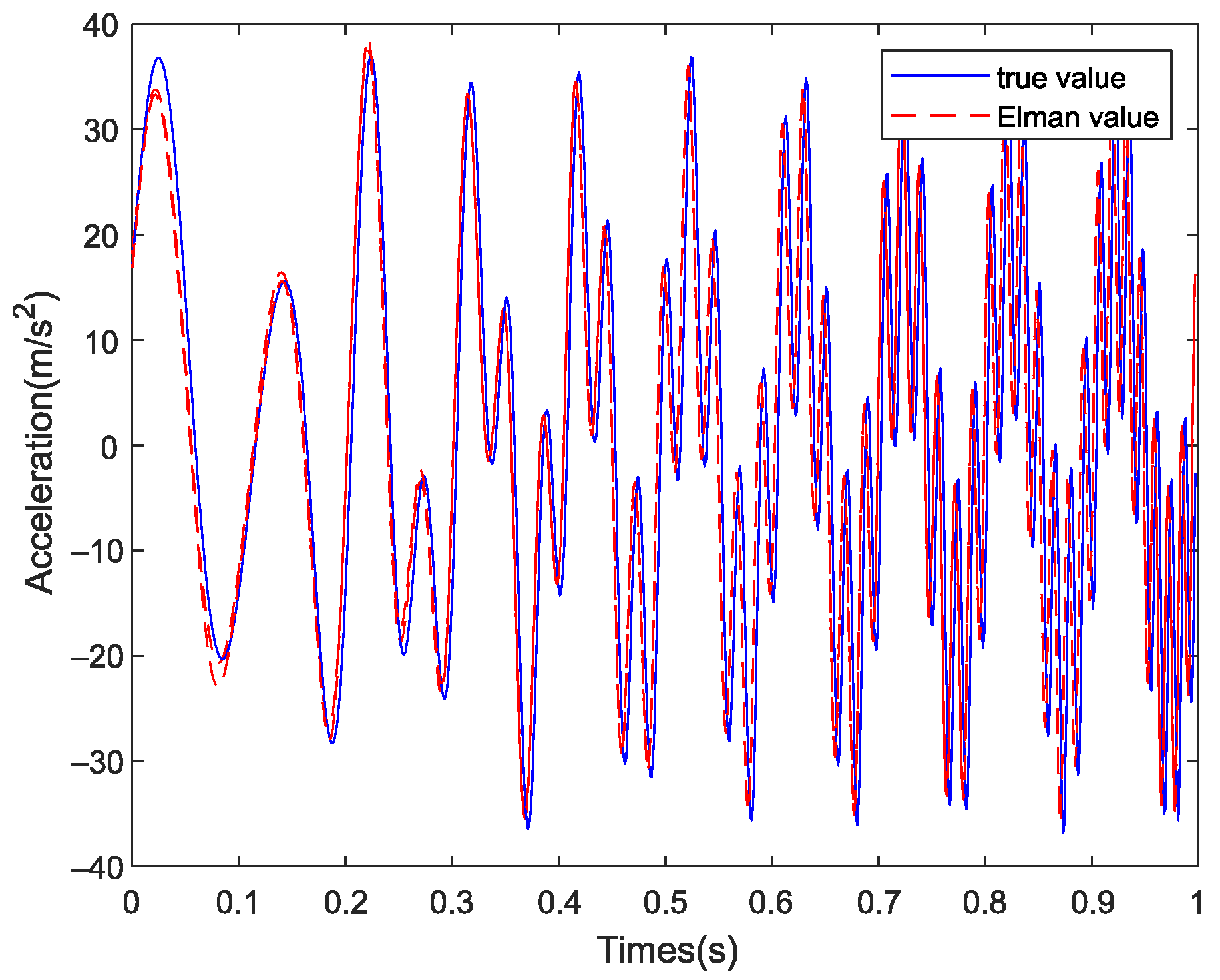
5. Experimental Results

In this section, the experimental results with the IEMD-ELM and EMD-ELM algorithms are presented. All the experiments were conducted on the test stand. The experimental data were sampled from the digital collection with a sampling frequency of 51.2 kHz and an analysis frequency of 20 kHz. The data acquisition equipment was the 3660C data acquisition instrument of B&K Company in Denmark. The main data acquisition parameters included vibration acceleration signal, noise signal, etc.

To verify the effectiveness of the proposed algorithm, the experiment data were sampled when a nonlinear load was applied in the system. The methods, including the IEMD-ELM algorithm and EMD-ELM algorithm, are compared in this section. The waveform of the input signal is shown in Figure 18.

Figure 18. The waveform of input signal.

The vibration characteristics of 1000 points were analyzed, and the waveform of the intercept signal is shown in Figure 19.

Figure 19. The waveform of intercept signal.

The decomposition efficiency of EMD and IEMD was compared by the orthogonality index, as shown in Table 5.

Table 5. Coefficients under different decomposition.

Method	Orthogonality Index
EMD	0.2437
IEMD	0.0660

As seen in Table 5, the orthogonality index of the EMD algorithm was 0.2437 and the orthogonality index of IEMD was 0.0660. Therefore, the IEMD algorithm is more complete than EMD decomposition. The effectiveness of the IEMD algorithm is verified.

IEMD and EMD algorithms were used to decompose the input signal. Figure 20 and Figure 21 show the corresponding decomposition patterns.

Figure 20. The EMD waveform of intercept signal.

Figure 21. The IEMD waveform of intercept signal.

Presented in Table 6 are the correlation coefficients between IMFs and input signals decomposed by the EMD algorithm and the IEMD algorithm. As defined by the correlation coefficient, the IEMD algorithm has a better decomposition effect than EMD algorithm.

Table 6. Coefficients under different decomposition.

Method	IMF1	IMF2	IMF3	IMF4	IMF5	IMF6	IMF7
EMD	0.90	0.10	0.20	0.19	0.04	−0.01	−0.02
IEMD	0.91	0.21	0.26	0.18	0.08	0.04	0.06

As shown in Table 6, the correlation coefficients of IMF1 and IMF2 were greater than the empirical threshold. However, the proportion of the effective signal component in the IEMD was larger than that in the EMD, so the effectiveness of the IEMD was verified. The reconstructed signal obtained using the decomposed effective IMF is shown in Figure 22.

Figure 22. The waveform of prediction signal.

The predicted signal is shown in Figure 22. The waveform predicted by the IEMD-ELM algorithm was in good agreement with the waveform trend of the original signal. The predicted value of the EMD-ELM algorithm was consistent with the waveform of the original signal, but the amplitude was offset. The comparison diagram can verify that the IEMD method has more decomposition and a higher reduction degree than the EMD method, which provides a new idea for hierarchical signal analysis.

6. Conclusions

In this paper, a combined algorithm based on IEMD and ELM is proposed to analyze and predict a diesel engine surface vibration signal. IEMD-ELM is used to decompose the surface vibration signal into a series of signal components, obtain the predicted value of corresponding signal components, and determine the characteristics of the surface vibration signal. Compared with EMD-ELM, IEMD-ELM predicts more accurately. In addition, in future work, our research will mainly focus on the following two points: (1) the adaptive decomposition part of the input surface vibration signal; and (2) fault study of input surface vibration signal.

References

1. Shen, Z.X.; Huang, X.Y.; Ma, X.X. Diesel engine fault diagnosis based on EMD and support vector machine. J. Vib. Meas. Diagn. 2010, 30. Available online: http://en.cnki.com.cn/Article_en/CJFDTotal-ZDCS201001006.htm (accessed on 24 September 2021).
2. Du, X.F.; Shu, G.Q.; Wei, H.Q.; Cao, X.-F. Influence law of diesel engine vibration source based on IMF sensitivity analysis. J. Tianjin Univ. Nat. Sci. Eng. 2015, 48, 1098–1104. [Google Scholar]
3. Wang, X.; Yue, Y.J.; Cai, Y.P. Fast Sparse Decomposition and Two-dimensional Feature Coding of Diesel Engine Vibration Signal Vibration. Chin. J. Test. Diagn. 2019, 39, 114–122, 225. [Google Scholar]
4. Xiao, B.; Shi, L.; Cao, Y.P. Source analysis of diesel engine based on adaptive generalized linear hybrid model. J. Harbin Eng. Univ. 2019, 40, 2029–2035. [Google Scholar]
5. Chen, D.; Wu, J.; Wang, L.; Liang, J.; Gong, X.; Kong, W. A method for predicting spindle rotation accuracy using vibration. Sci. Sin. Technol. 2020, 50, 819–828. [Google Scholar] [CrossRef]
6. Pang, C.S.; Liu, L.; Shan, T. Time-frequency analysis method based on short-time fractional Fourier transform. Acta Electron. Sin. 2014, 42, 347–352. [Google Scholar]
7. Shirkov, D.V. Fourier Transformation of the Renormalization-Invariant Coupling. Theor. Math. Phys. 2003, 136, 893–907. [Google Scholar] [CrossRef]
8. Li, H.; Zhang, Q.; Qin, X.R. Bearing fault diagnosis method based on STFT and convolutional neural network. J. Vib. Shock. 2018, 37, 124–131. [Google Scholar]
9. Xu, Y.G.; Meng, Z.P.; Zhao, G.L. Study on compound fault diagnosis of rolling bearing based on dual-tree complex wavelet transform. Chin. J. Sci. Instrum. 2014, 35, 447–452. [Google Scholar]
10. Chen, R.X.; Huang, X.; Yang, L.X. Rolling bearing fault diagnosis based on convolutional neural network and discrete wavelet transform. J. Vib. Eng. 2018, 31, 883–891. [Google Scholar]
11. Wu, Z.; Huang, N.E. A study of the characteristics of white noise using the empirical mode decomposition method. Proc. R. Soc. A Math. Phys. Eng. Sci. 2004, 460, 1597–1611. [Google Scholar] [CrossRef]
12. Lei, Y.; Lin, J.; He, Z. A review on empirical mode decomposition in fault diagnosis of rotating machinery. Mech. Syst. Signal Process. 2013, 35, 108–126. [Google Scholar] [CrossRef]
13. Huang, N.E. Introduction to the Hilbert-Huang Transform and its Related Mathematical Problems. In Hilbert-Huang Transform and Its Applications; Huang, N.E., Shen, S.S.P., Eds.; World Scientific: Singapore, 2005. [Google Scholar]
14. Xiao, Y.; Yin, F.L. De-correlation EMD: A new method of eliminating mode mixing. J. Vib. Shock. 2015, 34, 25–29. [Google Scholar]
15. Hu, A.J.; Sun, J.J.; Xiang, L. Modal Aliasing problem in Empirical Mode Decomposition. Vib. Chin. J. Meas. Diagn. 2011, 31, 429–434, 532–533. [Google Scholar]
16. Bai, C.H.; Zhou, X.C.; Lin, D.C. Research on PSO-SVM method for eliminating EMD endpoint effect. Syst. Eng. Theory Pract. 2013, 33, 1298–1306. [Google Scholar]
17. He, Z.P.; Zhu, Z.Q.; Xie, H.C.; Wang, Y.; Li, Z.; He, R.; Du, C.; Li, J. Restrain Boundary Effect of EMD Based on Least Square Fitting. J. Syst. Simul. 2018, 30, 3377. [Google Scholar]
18. Hu, L.P.; Song, E.L.; Li, B.Q. A fast EMD algorithm for stream data analysis. J. Vib. Shock. 2012, 31, 116–120. [Google Scholar]
19. Li, X.Y.; Zou, X.J.; Zhang, R.B.; Qian, Z. Research on empirical mode decomposition based on spectrum entropy methods and principal component analysis. J. Harbin Eng. Univ. 2009, 30, 797–803. [Google Scholar]
20. Tang, B.; Dong, S.; Song, T. Method for eliminating mode mixing of empirical mode decomposition based on the revised blind source separation. Signal Process. 2012, 92, 248–258. [Google Scholar] [CrossRef]
21. Kurbatskii, V.G.E.; Sidorov, D.N.; Spiryaev, V.A.; Tomin, N.V. On the neural network approach for forecasting of nonstationary time series on the basis of the Hilbert–Huang transform. Autom. Remote Control 2011, 72, 1405–1414. [Google Scholar] [CrossRef]
22. Hu, X.Y.; Peng, S.L.; Tan, J. Back projection strategy for solving mode mixing problem. Int. J. Wavelets Multiresolut. Inf. Process. 2012, 10, 1250031. [Google Scholar] [CrossRef]
23. Hu, N.Q.; Chen, H.P.; Cheng, Z.; Zhang, L. Fault Diagnosis Method of Planetary Gearbox Based on Empirical Mode Decomposition and Deep Convolutional Neural Network. Chin. J. Mech. Eng. 2019, 55, 9–18. [Google Scholar] [CrossRef] [Green Version]
24. Kurbatskii, V.G.; Sidorov, D.N.; Spiryaev, V.A.; Tomin, N.V. Tomin Forecasting nonstationary time series based on Hilbert–Huang transform and machine learning. Autom. Remote Control 2014, 75, 922–934. [Google Scholar] [CrossRef]
25. Xu, K.; Chen, Z.H.; Zhang, C.B. Rolling bearing fault diagnosis based on empirical mode decomposition and support vector machine. Control Theory Appl. 2019, 36, 915–922. [Google Scholar]
26. Leung, T.; Zhao, T. Financial Time Series Analysis and Forecasting with HHT Feature Generation and Machine Learning. Appl. Stoch. Models Bus. Ind. 2021. [CrossRef]
27. Mishra, M.; Panigrahi, R.R. Advanced signal processing and machine learning techniques for voltage sag causes detection in an electric power system. Int. Trans. Electr. Energy Syst. 2020, 30, e12167. [Google Scholar] [CrossRef]
28. Parkavi, R.M.; Shanthi, M.; Bhuvaneshwari, M.C. Recent trends in ELM and MLELM: A review. Adv. Sci. Technol. Eng. Syst. J. 2017, 2, 69–75. [Google Scholar] [CrossRef] [Green Version]
29. Xu, R.; Liang, X.; Qi, J.S. Advances and trends of extreme learning machine. Chin. J. Comput. Mach. 2019, 42, 1640–1670. [Google Scholar]
30. Huang, G.B.; Zhu, Q.Y.; Siew, C.K. Extreme learning machine: Theory and applications. Neurocomputing 2006, 70, 489–501. [Google Scholar] [CrossRef]
31. Ding, S. Extreme learning machine: Algorithm, theory and applications. Artif. Intell. Rev. 2015, 44, 103–115. [Google Scholar] [CrossRef]
32. Zhao, Z.; Zhang, X. Theory and Numerical Analysis of Extreme Learning Machine and Its Application for Different Degrees of Defect Recognition of Hoisting Wire Rope. Shock Vib. 2018, 2018, 4168209. [Google Scholar] [CrossRef]