Evaluation of Energy Price Liberalization in Electricity Industry: A Data-Driven Study on Energy Economics

Abstract

This study aims to evaluate the effects of price liberalization on energy consumption intensity, because price liberalization leads to improved productivity, energy consumption management, and consumption reform. Although the energy consumption of large-scale factories and industries has increased dramatically, and the energies losses have an increment in the power transmission lines, this policy can result in decreasing the energy consumption intensity due to the changes in consumption patterns. If there is a correlation between two variables, the price can be a valid variable to control cost and increase consumption efficiency. The augmented Dickey–Fuller (ADF) and the Chi-squared tests are also employed to investigate the maneuverability of these variables in the first-order contrast. In this case study, the energy consumption intensity response to price changes using the data gathered between 1988–2020, has gained a confidence interval of these reactions at 95%. The proposed vector autoregressive (VAR) model has forecasted the action and reaction of the end-user, to investigate the future shocks between 2020–2050, considering a new price shock, in the Iranian energy market for the first time. The research findings have shown that energy price liberalization leads to the energy intensity improvement, however, the end-user (shocking) reactions should be investigated to implement a more sustainable policy that eases the new energy price rises.

1. Introduction

1.1. Research Challenge

Electricity has an intrinsic and determinant role in economic evolution. The economic expansion and industrialization process have increase energy demand and energy consumption intensity. Therefore, energy price liberalization is considered a critical issue for policymakers and financial planners. Electricity, due to unique characteristics, has been used incomparable to another sources of energy worldwide. At the end of the fifth developed program, the states have to reduce energy intensity concerning energy price liberalization. Growing energy consumption in many countries, and their trend lead to reducing this growth in consumption [1,2,3]. The studies have shown that the figure of energy consumption in industries and the high-energy consumption of electricity used in equipment, high electricity losses in transmission and distribution, lack of culture, and low energy prices, especially in manufacturing enterprises, have caused increasing energy intensity. The plan price energy liberalization was approved in January 2009, which was affected by economic, cultural, and social aspects [4]. All businesses are directly and indirectly affected by the project, particularly the energy used in industries. According to reports on the amount of electricity consumption, and comparing it with after implementation of this policy, has been one of the primary purposes is raising efficiency, energy consumption management, and modified energy consumption in enterprises [5,6,7]. These policies have directly influenced the end-user (customers) energy consumption intensity, which should be studied to observe the dynamic (instability and stability) trends for price liberalization purposes.

1.2. Literature Review

Related studies [8,9,10,11,12,13,14,15,16,17,18,19,20,21,22,23,24,25,26,27,28,29,30,31,32,33,34,35,36,37,38,39,40,41,42] have been conducted on the effects of price liberalization and subsidies orientation and the effects on economic growth, for example:

Štefan Bojnec and Alan Križaj [11], analyzed the electricity markets for market deregulation and price liberalization, in Slovenia. They studied the impacts of the electricity prices and electricity consumption for a specific period. Based on their empirical research outcome, the authors explained the importance of both internal domestic and external regional and international driving forces for the formation of electricity prices and their implications on electricity consumption in both industry and residential sectors. The single energy market is the core of today’s EU economy, where households and businesses can choose their supplier of energy (e.g., electricity and natural gas). They also found that the higher electricity consumption is, the more increases in electricity prices can be seen if the production and supply of electricity do not follow the increase in demands.

In another study [12], the researchers analyzed the impacts of natural resources, energy consumption and gross capital accumulation on economic growth over a period in more than a hundred countries classified based on various income levels (i.e., low, middle and high income) using panel vector autoregressive (PVAR) method. Interestingly, they found a relationship between the economic development and the energy consumption in high-income countries, considering their capital formation. Finally, the authors provided some suggestions for policymakers based on their level of income.

Abdul Rehman and et al. [13], studied the impacts of information and communication technology, based on the time series data between 1985–2017. To do this, they employed ADF test method, when an autoregressive distributed lag (ARDL) model has been utilized to evaluate the dynamic association amid prescribed variables with both short-term and long-term analyses. They have found some interesting relationships among the studied variables, for example, the trade and renewable energy. Both variables played significant impacts on the GDP, whereas the foreign direct investment has shown a harmful effect on the GDP growth. The researchers have also proposed some recommendations for the policymakers.

In the reference [14], the researchers analyzed the effects of economic uncertainty on structural shocks to global oil supply, aggregate demand, and energy consumption. The authors studied both linear/nonlinear impulse responses of economic uncertainty to oil price changes in a large number of economies using local projection approaches. They have found that the sudden changes in oil consumption could be seen as positive news for lowering the economic uncertainty. Finally, the authors provided some suggestions for policymakers in financial markets.

Zhao Xin-gang et al. [15], presented the development process of marketization and the changes in energy efficiency affected by electricity prices. They have found that stabilization of the electricity price and energy efficiency can affect the energy efficiency improvement in a long-term. Under positive and/or negative shocks, the impulse response is reported opposite, with longer response mainly under the positive shock. The authors have also proposed some policy implications on their findings for improving the electricity price.

In [16], the authors studied the impacts of energy cost liberalization policies on the of wind farms compared to gas power plants. They reported that such a policy can support this type of power plant to operate cost-effective in developing countries such as Iran. In a similar investigation, the authors [17] have evaluated the causality and effects of several variables such as electricity consumption, economic growth, and capital stock. To predict these variables and to offer the corresponding policy needed in Iran. To discuss their findings, they have employed several mathematical methods such as VAR and Bayesian information criterion (BIC) for prediction and statistical analyses.

In [18], Bahareh Oryani, et al., evaluated the effects of produced renewable energy on economic development and CO₂ emission reduction, between 1980–2016. To do this, the authors have employed structural VAR and impulse response function for their predictions. Interestingly, they have reported that in this stage of the country development, investing more in the renewable energy production cannot be a suitable scenario to control environmental-related concerns. Instead, they have proposed some policy-focused amendments such as better monitoring systems.

More technical papers on electricity market forecasting, energy consumption and price can be found in [19,20,21], in which worldwide viewpoints discussed.

The economic and econometric times series are based on the static assumption variables. Hence, the mean and variance throughout the period are constant. Based on studies after 1990, this assumption is incorrect, and most of these variables are time-dependent and unambiguous [22]. Studies have shown that if the variables in time series are non-stationary using t and F tests, which can be misleading. The results are more likely to represent a false regression and no accurate economic equilibrium relationship between the variables. Therefore, it is vital to assess the stationary or non-stationary time series variables to avoid fake regressive [23].

Vector autoregressive (VAR) model has been considered an essential model to predict macro-econometric issues, while using this model to policy assess is controversial. There is more advantage in developing countries; this approach has no previous limitation; at least, comparing results can be helpful to VAR modeling. Each variable has an equation explaining its evolution based on its own lagged values. Due to the many variables, the model has a vector. Due to the emergence of the dependent variable with their lags, the model is autoregressive [11,12,18,24,29,32].

In this paper, the main task is to analyze the impacts of price liberalization on energy consumption intensity, in the Iran market for the first time. Since price liberalization leads to improved productivity, energy consumption management, and consumption reform. To do this, the researchers used the historic data, between 1988–2020, reported by the Iranian Ministry of Energy. To fit the estimation model, the historic data on energy consumption intensity, GDP, labor, capital, and energy prices (i.e., electricity, diesel, oil, and gas) are defined as variables. The energy price liberalization policy has whatsoever a significant influence in decreasing the energy consumption intensity, because of the changes in consumption patterns. If there is a correlation between two variables, the price-related variables are significant to control cost and improve the consumption efficiency. Using the augmented Dickey–Fuller (ADF) and the Chi-squared tests, variables on their first-order difference indicate the maneuverability of these variables in the first-order contrast. In this case study, the energy consumption intensity response to price changes, and the confidence interval of these reactions is at the 95% confidence level, for Iran energy market. Considering the effects of price liberalization on energy consumption intensity in the electrical-based industries. In this work, the study is initiated based on fractional co-integrated methods [25], and then the long-term equation is estimated. As a main research contribution, a VAR model, based on the data, is developed to analyze the action, reaction, and shocks in the future period. The general framework of the research is:

$${\mathrm{Y}}_{\mathrm{t}}=\mathsf{\alpha }+{\mathsf{\beta }}_1{\mathrm{Y}}_{\mathrm{t}-1}+\cdots +{\mathsf{\beta }}_{\mathrm{p}}{\mathrm{Y}}_{\mathrm{t}-\mathrm{p}}+{\mathsf{\gamma }\mathrm{D}}_{\mathrm{t}}+{\mathsf{\epsilon }}_{\mathrm{t}}$$

(1)

where Y indicates endogenous variables, and $\mathrm{n}\times 1$ vector, p is lag order in the VAR model. D is a valid quality variable on the dependent variable and $\mathsf{\epsilon }$ defined vector error terms. The Y vector contains energy intensity in the electricity industry, energy price, value-added, and other variables in this research.

Note that energy consumption intensity (units of energy per unit of GDP) is a measurer for studying how an economy might be unhealthy. In an unhealthy economy, high levels of energy consumption intensity show a high price of shifting the energy to GDP improvement. On the other hand, the low levels of the energy consumption intensity have lower cost of shifting the energy to GDP can be reported, which often happens in the healthier economies.

2. Proposed Methodology and Mathematical Modeling

2.1. Research Taxonomy

In this section, the estimation modeling methods alongside the framework of the proposed methodology are defined. To allow the experts to follow the steps taken in this study, the framework consists of the following steps:

• Step 1: Defining the specification of the variables, for more details see Table 1;
• Step 2: Studying the static level of time series data using ADF test method, for more details see Table 2 and Table 3, where Table 3 determines the variables are stationary in the first level;
• Step 3: Determining optimal lag length with three criteria, in which the optimal lag is set two in this work, see Table 4;
• Step 4: Estimating the pre-defined variables in the VAR model that calculates and analyze how variables affect each other, more details can be found in Table 5;
• Step 5: Introducing a new price increase (or impulse), based on the real-life policy made in Iran to remove considerable energy-related subsides, for investigating its impacts on the energy intensity and the end-user reactions. Analyzing impulsive response function (IRF) trend to obtain policy viewpoints, which resulted in Figure 1, Figure 2, Figure 3 and Figure 4;
• Step 6: Finding long term relationship between variables by Johansen co-integration model with maximum engine value and trace tests, see Table 6 and Table 7;
• Step 7: Normalization of the co-integrated vector to interpret estimation results using Equation (28) and develop a long-term relationship, results in Table 8;
• Step 8: Estimating VECM to discover the variables convergence, due to the VECM coefficient set 0.15, more details can be seen in Table 9;

Required datasets consisting of several variables to fit the estimation model are collected between the period of 1988 to 2020 annually to evaluate the influence of price liberalization. These variables are energy consumption intensity, GDP, labor, capital, and price of substitute goods obtained from the Central Bank of Iran, Department of Economic Time Series Database [43], and Iran Statistics Center [44]. For this study, the prices of energy resources are fixed as 1 kWh of electricity = 0.045$, 1 L of oil = 0.071$, 1 m³ of gas = 0.054$, and 1 m³ of diesel = 0.071$, all the values are reported by the Energy Ministry of Iran, see [4] for more details.

In this work, the evaluation and prediction of the effect of price liberalization on energy consumption are studied for the first time, in Iran. To do this, first, the data should be stationary, then discovering the co-integrated relations after finding the optimal lag. Finally, forecast the influence of this policy in the future.

2.2. Vector Autoregressive (VAR) Model

In this work, the multivariate time series model, such as the VAR model, attempts to provide a variable’s response based on the previous values and several variables simultaneously [26]. The variables of the VAR model are defined as a function of their intermittent values, other variables, and random components such as ${\mathsf{\epsilon }}_{\mathrm{t}}$. In traditional methods, first, the variables are divided into two categories of intrinsic and extrinsic, at the same time. Whereas in the VAR method, such a determination is not required. Still, there is no need to optionally separate the variables into intrinsic and extrinsic, as in traditional methods. The VAR does not have any implicit theoretical basis. Therefore, they are more useful when the theoretical foundations of the subject under study are not strong enough. However, the VAR model has explained its evolution based on its own lagged values and error terms. None of the coefficient matrices is zero. In other words, all restrictions, which lay on the coefficients model, are non-zero quantities [27].

The use of the VAR models has brought the following features into the investigation:

• Etiological can conduct economies with times series, this method has been used in macroeconomics in developing countries.
• Examining economic shocks to evaluate shocks is another considerable advantage. Since every economy can be affected differently, due to these shocks.
• The third benefit is the variance variable during the period related to the second application of this method. It means how each variable can influence on the other variables.
• In the VAR method used, all the variables are considered intrinsic.
• The VAR models have shown a better estimation than a sophisticated equation or ordinary least squares (OLS), see [28,29].

$$\begin{gathered} {\mathrm{U}}_{\mathrm{t}}\approx \mathrm{N}\left(0,\mathsf{\sigma }\right) \\ {\mathrm{Y}}_{\mathrm{it}}={\mathrm{A}}_1{\mathrm{Y}}_{\mathrm{i}.\mathrm{t}-1}+\cdots +{\mathrm{A}}_{\mathrm{p}}{\mathrm{Y}}_{\mathrm{i}.\mathrm{t}-\mathrm{p}}+{\mathrm{U}}_{\mathrm{it}} \end{gathered}$$

(2)

where Y_it is the output model with endogenous variables, A_i (i = 1, …, p) is the coefficient K × K matrix, in which p is lag order in this model. In addition, U_it is a K × 1 vector that is error vector with normal distribution with zero average. In this model, each Y_t variable is solved according to a lag of its variable and other endogenous variables. In ordinary least square methods, the coefficients can be estimated efficiently. The reason is that the right variable of the equation has been predictive and the same exactly. Additionally, if there is more than one co-integrate vector, the Engel-Granger method, which is unsuitable for this kind of analysis [30,31]. Finally, the Johansen Juselius method [32] estimates the cointegrating vector based on the maximum likelihood vector [32,33].

2.3. Determining the Optimal Lag

The optimal lag determined by the criteria of Akaike, shown as AIC [34], Schwarz-Bayesian, presented as SBC [35,36] and Hanan Quinn [36], indicated as HQC in the paper. Their fundamental equations are given as:

$$\mathrm{AIC}=\ln (\hat{\mathsf{\theta }})-\mathrm{P}$$

(3)

$$\mathrm{SBC}=\ln (\hat{\mathsf{\theta }})-\frac{1}{2}\mathrm{P}.\log (n)$$

(4)

$$\mathrm{HQC}=\ln (\hat{\mathsf{\theta }})-(\log \log n)\mathrm{P}$$

(5)

In these relationships, $\ln (\hat{\mathsf{\theta }})$ is the maximum likelihood function in an econometric model, where $\hat{\mathsf{\theta }}$ is the maximum likelihood estimation of coefficients, P contains the estimated parameters, n is a sample size, and the maximum amount of z represented the number of optimal lags [32].

Determining optimal dependent variables for regression and elimination of the correlation between disturbance terms, among all three criteria (AIC, SBC, and HQC), see [34,35,36,37]. It is likely to obtain different lags which can result in uncommon answers.

2.4. Impulsive Response Function (IRF)

The function responds to an endogenous variable resulting from a change in disturbance variable or time. For example, when there are two endogenous variables in the autoregressive vector, four response functions have existed in this regard. Finally, only one shock with standard deviation can affect the price variation [33,38,39]. It is validated that an autoregressive equation has turned into a moving average equation, and vice versa [40,41,42].

$$\left[\begin{array}{cc}1& {\mathrm{b}}_{12}\\ {\mathrm{b}}_{21}& 1\end{array}\right]\left[\begin{array}{c}{\mathrm{y}}_{\mathrm{t}}\\ {\mathrm{z}}_{\mathrm{t}}\end{array}\right]=\left[\begin{array}{c}{\mathrm{b}}_{10}\\ {\mathrm{b}}_{20}\end{array}\right]+\left[\begin{array}{cc}{\mathsf{\gamma }}_{11}& {\mathsf{\gamma }}_{12}\\ {\mathsf{\gamma }}_{21}& {\mathsf{\gamma }}_{22}\end{array}\right]\left[\begin{array}{c}{\mathrm{y}}_{\mathrm{t}-1}\\ {\mathrm{z}}_{\mathrm{t}-1}\end{array}\right]+\left[\begin{array}{c}{\mathsf{\epsilon }}_{\mathrm{yt}}\\ {\mathsf{\epsilon }}_{\mathrm{zt}}\end{array}\right]$$

(6)

Alternatively, ${\mathrm{Bx}}_{\mathrm{t}}={\mathsf{\Gamma }}_0+{\mathsf{\Gamma }}_1{\mathrm{x}}_{\mathrm{t}-1}+{\mathsf{\epsilon }}_{\mathrm{t}}$ is such that:

$$\mathrm{B}=\left[\begin{array}{cc}1& {\mathrm{b}}_{12}\\ {\mathrm{b}}_{21}& 1\end{array}\right],{\mathrm{X}}_{\mathrm{t}}=\left[\begin{array}{c}{\mathrm{y}}_{\mathrm{t}}\\ {\mathrm{z}}_{\mathrm{t}}\end{array}\right],{\mathsf{\Gamma }}_0=\left[\begin{array}{c}{\mathrm{b}}_{10}\\ {\mathrm{b}}_{20}\end{array}\right],{\mathsf{\Gamma }}_1=\left[\begin{array}{cc}{\mathsf{\gamma }}_{11}& {\mathsf{\gamma }}_{12}\\ {\mathsf{\gamma }}_{21}& {\mathsf{\gamma }}_{22}\end{array}\right],{\mathsf{\epsilon }}_{\mathrm{t}}=\left[\begin{array}{c}{\mathsf{\epsilon }}_{\mathrm{yt}}\\ {\mathsf{\epsilon }}_{\mathrm{zt}}\end{array}\right]$$

(7)

where X_t is the matrix of current and future values, B is the identity matrix, Γ₁ is the linear coefficients and Γ₀ is the independent matrix and ${\mathsf{\epsilon }}_{\mathrm{t}}$ is the error values Then the standard form of autoregressive can be given as:

$${\mathrm{x}}_{\mathrm{t}}={\mathrm{A}}_0+{\mathrm{A}}_1{\mathrm{x}}_{\mathrm{t}-1}+{\mathrm{e}}_{\mathrm{t}}$$

(8)

where, the coefficients are computed based on:

$$\begin{gathered} {\mathrm{A}}_0={\mathrm{B}}^{-1}{\mathsf{\Gamma }}_0 \\ {\mathrm{A}}_1={\mathrm{B}}^{-1}{\mathsf{\Gamma }}_1 \end{gathered}$$

(9)

$${\mathrm{e}}_{\mathrm{t}}={\mathrm{B}}^{-1}{\mathsf{\epsilon }}_{\mathrm{t}}$$

The convertor of a vector moving average is as follows, in which y_t and z_t variables are current (e_1t) and future (e_2t) values, respectively.

$${\mathrm{x}}_{\mathrm{t}}=\mathsf{\mu }+{{\displaystyle \sum }}_{\mathrm{i}=0}^{\infty }{\mathrm{A}}_1^{\mathrm{i}}{\mathrm{e}}_{\mathrm{t}-\mathrm{i}}$$

(10)

where $\mathsf{\mu }$ is the mean vector of y and z, as given below:

$$\mathsf{\mu }={\left[\stackrel{\_}{\mathrm{y}}\stackrel{\_}{\mathrm{z}}\right]}^{\prime }$$

(11)

$$\stackrel{\_}{\mathrm{y}}=\frac{\left[{\mathrm{a}}_{10}\left(1-{\mathrm{a}}_{22}\right)+{\mathrm{a}}_{12}{\mathrm{a}}_{20}\right]}{\Delta }$$

(12)

$$\stackrel{\_}{\mathrm{z}}=\frac{\left[{\mathrm{a}}_{20}\left(1-{\mathrm{a}}_{11}\right)+{\mathrm{a}}_{21}{\mathrm{a}}_{10}\right]}{\Delta }$$

(13)

$$\Delta =\left(1-{\mathrm{a}}_{11}\right)\left(1-{\mathrm{a}}_{22}\right)-{\mathrm{a}}_{12}{\mathrm{a}}_{21}$$

(14)

A feature vector moving average method [18] analyzes the shocks that impose on the VAR variables. To further explain this, the VAR model considers two variables, and the matrix form is as follow:

$$\left[\begin{array}{c}{\mathrm{y}}_{\mathrm{t}}\\ {\mathrm{z}}_{\mathrm{t}}\end{array}\right]=\left[\begin{array}{c}{\mathrm{a}}_{10}\\ {\mathrm{a}}_{20}\end{array}\right]+\left[\begin{array}{cc}{\mathrm{a}}_{11}& {\mathrm{a}}_{12}\\ {\mathrm{a}}_{21}& {\mathrm{a}}_{22}\end{array}\right]\left[\begin{array}{c}{\mathrm{y}}_{\mathrm{t}-1}\\ {\mathrm{z}}_{\mathrm{t}-1}\end{array}\right]+\left[\begin{array}{c}{\mathrm{e}}_{1\mathrm{t}}\\ {\mathrm{e}}_{2\mathrm{t}}\end{array}\right]$$

(15)

using the Equation (4), the equation can be rewritten as:

$$\left[\begin{array}{c}{\mathrm{y}}_{\mathrm{t}}\\ {\mathrm{z}}_{\mathrm{t}}\end{array}\right]=\left[\begin{array}{c}\stackrel{\_}{\mathrm{y}}\\ \stackrel{\_}{\mathrm{z}}\end{array}\right]+{{\displaystyle \sum }}_{\mathrm{i}=0}^{\infty }{\left[\begin{array}{cc}{\mathrm{a}}_{11}& {\mathrm{a}}_{12}\\ {\mathrm{a}}_{21}& {\mathrm{a}}_{22}\end{array}\right]}^{\mathrm{i}}\left[\begin{array}{c}{\mathrm{e}}_{1\mathrm{t}-\mathrm{i}}\\ {\mathrm{e}}_{2\mathrm{t}-\mathrm{i}}\end{array}\right]$$

(16)

In the Equation (16), Variables, y_t, and z_t have defined in terms of sequence of ε_zt and ε_yt. Since if the equation has written base on this sequence is better in this regard. The error vector has written the Equation (10):

$${\mathrm{e}}_{1\mathrm{t}}=\frac{\left({\mathsf{\epsilon }}_{\mathrm{yt}}-{\mathrm{b}}_{12}{\mathsf{\epsilon }}_{\mathrm{zt}}\right)}{\left(1-{\mathrm{b}}_{12}{\mathrm{b}}_{21}\right)}$$

(17)

$${\mathrm{e}}_{2\mathrm{t}}=\frac{\left({\mathsf{\epsilon }}_{\mathrm{zt}}-{\mathrm{b}}_{21}{\mathsf{\epsilon }}_{\mathrm{yt}}\right)}{\left(1-{\mathrm{b}}_{12}{\mathrm{b}}_{21}\right)}$$

(18)

$$\left[\begin{array}{c}{\mathrm{e}}_{1\mathrm{t}}\\ {\mathrm{e}}_{2\mathrm{t}}\end{array}\right]=\frac{1}{1-{\mathrm{b}}_{12}{\mathrm{b}}_{21}}\left[\begin{array}{cc}1& -{\mathrm{b}}_{12}\\ -{\mathrm{b}}_{21}& 1\end{array}\right]\left[\begin{array}{c}{\mathsf{\epsilon }}_{\mathrm{yt}}\\ {\mathsf{\epsilon }}_{\mathrm{zt}}\end{array}\right]$$

(19)

Therefore, the Equations (15) and (16) are combined and written as below:

$$\left[\begin{array}{c}{\mathrm{y}}_{\mathrm{t}}\\ {\mathrm{z}}_{\mathrm{t}}\end{array}\right]=\left[\begin{array}{c}{\stackrel{\_}{\mathrm{y}}}_{\mathrm{t}}\\ {\stackrel{\_}{\mathrm{z}}}_{\mathrm{t}}\end{array}\right]+\frac{1}{1-{\mathrm{b}}_{12}{\mathrm{b}}_{21}}{{\displaystyle \sum }}_{\mathrm{i}=0}^{\infty }{\left[\begin{array}{cc}{\mathrm{a}}_{11}& {\mathrm{a}}_{12}\\ {\mathrm{a}}_{21}& {\mathrm{a}}_{22}\end{array}\right]}^{\mathrm{i}}\left[\begin{array}{cc}1& -{\mathrm{b}}_{12}\\ -{\mathrm{b}}_{21}& 1\end{array}\right]\left[\begin{array}{c}{\mathsf{\epsilon }}_{\mathrm{yt}-\mathrm{i}}\\ {\mathsf{\epsilon }}_{\mathrm{zt}-\mathrm{i}}\end{array}\right]$$

(20)

Due to a simple system, the matrix φ_i in which components are φ_jk(0) is defined as:

$${\mathsf{\phi }}_{\mathrm{i}}=\frac{{\mathrm{A}}_1^{\mathrm{i}}}{1-{\mathrm{b}}_{12}{\mathrm{b}}_{21}}\left[\begin{array}{cc}1& -{\mathrm{b}}_{12}\\ -{\mathrm{b}}_{21}& 1\end{array}\right]$$

(21)

Therefore, the vector moving average equations of (6) and (10) are a function of ε_zt and ε_yt, which can be given as:

$$\left[\begin{array}{c}{\mathrm{y}}_{\mathrm{t}}\\ {\mathrm{z}}_{\mathrm{t}}\end{array}\right]=\left[\begin{array}{c}\stackrel{\_}{\mathrm{y}}\\ \stackrel{\_}{\mathrm{z}}\end{array}\right]+{{\displaystyle \sum }}_{\mathrm{i}=0}^{\infty }{\left[\begin{array}{cc}{\mathsf{\phi }}_{11}\left(\mathrm{i}\right)& {\mathsf{\phi }}_{12}\left(\mathrm{i}\right)\\ {\mathsf{\phi }}_{21}\left(\mathrm{i}\right)& {\mathsf{\phi }}_{22}\left(\mathrm{i}\right)\end{array}\right]}^{\mathrm{i}}\left[\begin{array}{c}{\mathsf{\epsilon }}_{\mathrm{yt}-\mathrm{i}}\\ {\mathsf{\epsilon }}_{\mathrm{zt}-1}\end{array}\right]$$

(22)

which can be simplified as:

$${\mathrm{x}}_{\mathrm{t}}=\mathsf{\mu }+{{\displaystyle \sum }}_{\mathrm{i}=0}^{\infty }{\mathsf{\phi }}_{\mathrm{i}}{\mathsf{\epsilon }}_{\mathrm{t}-\mathrm{i}}$$

(23)

Vector autoregressive moving average is considered a practical approach to evaluate the relation between y_t and z_t. Using the matrix coefficient φ_i, it has assessed the effect of the shocks of ε_yt and ε_zt on the whole time series y_t and z_t. It is obvious that the four array of matrix φ_i shows that φ_ijk(0) considered ascending coefficient shocks. For example, coefficient φ₁₂(0) represents the instant shocks of changing a unit of ε_zt on y_t any way the values of φ₁₁(1) and φ₁₂(1) represented the effect of one-unit change of ε_yt-1 and ε_zt-1 on y_t throughout a period.

Assuming that the equation changes one unit forward, the values φ₁₁(1) and φ₁₂(1) represented the effect of a unit change in ε_yt and ε_zt on y_t+1, respectively. The overall effect of a single impulse unit on ε_yt or ε_zt is a two-variables model that may be the sum of coefficients impulse response obtained. For instance, the effect of a single impulse unit on ε_zt after n period on y_t+n can result in φ₁₂(n). Hence, the result of the overall effect of ε_zt on the sequence y_t after n period can be given as:

$${{\displaystyle \sum }}_{\mathrm{i}=0}^{\mathrm{n}}{\mathsf{\phi }}_{12}\left(\mathrm{i}\right)$$

(24)

2.5. Johansen Juselius Method

Johansen Juselius method, see more details in [32], has considered a prominent way of analyzing the relationship between the variables and the estimated long-term relationship. In recent years, it has been an essential tool to determine time-series economic variables. The relation between VAR and converge possible way to an obtained autoregressive coefficient [27]. Convergence vectors have been obtained from the autoregressive coefficient as follow:

(1)

making VAR coefficient matrix, which is known as A matrix;

(2)

characteristic root matrix, known as λ, resulted from the characteristic equation defined as:

$$\left|\mathrm{A}-\mathsf{\lambda }\mathrm{I}\right|=0$$

(25)

(3)

each characteristic vector has calculated from the characteristic root matrix, given as:

$$\left(\mathrm{A}-\mathsf{\lambda }\mathrm{I}\right)\mathrm{C}=0$$

(26)

(4)

the R matrix has formed and the inverse matrix is calculated, then the row that associated with the non-unit root $\mathsf{\lambda }<1$ is represented as a converge vector.

The mathematical form of the vector regression model is:

$${\mathrm{Y}}_{\mathrm{t}}=\mathrm{A}+{{\displaystyle \sum }}_{\mathrm{p}=1}^{\mathsf{\tau }}{\mathrm{B}}_{\mathrm{p}}{\mathrm{Y}}_{\mathrm{t}-\mathrm{p}}+{\mathrm{E}}_{\mathrm{t}}$$

(27)

where Y is a vector consisting of some variables within the existing model, $\mathsf{\tau }$ is delay lag, A is an intercept of vector component of the equation, and E is a vector of random error elements which are normally distributed with constant mean and zero variance.

3. Data Analysis and Discussion

For the data analysis, the statistical characteristics of the studied variables are evaluated. The findings of the statistical test have estimated the model used in this work. Moreover, the influence of energy price liberalization on the research variables and long-term relationships are studied, based on the data published by [4,43,44], for the first time. For example, Iran’s electricity generation capacity has been reported 68,932 MW, which has been increased by 3720 MW, in 2018. Thermal power has been generated 57,541 MW, and 20 MW is related to a nuclear power plant. From hydroelectricity generated 9686 MW (ranked third). In addition, the capacity of renewable energy and small power plant has been reported 219 MW and 466 MW, respectively. Total energy produced in power plants is at 248.595000 TW in 2018, which consumed 37,506 × 106 m³ gas, 7659 × 106 L of gasoline, and 14,441 × 106 L oil. Electricity import in 2014 has been grown 7% compared to the 2013 year, but electricity export has been increased by 28%. In 2018, the energy consumption has been reported at 3345 kWh, and energy production at 2553 kWh, for which domestic use is 2622 kWh, more information can be found in [33].

3.1. Statistical Specification Variables

Some specifications, such as maximum, minimum, mean, standard deviation, and skewness and elongation, are presented in Table 1. As given in the table, the energy consumption intensity based on kJ/$, gross domestic product (GDP) based on $, labor, capital stock, and price of energy are computed. For example, one of the most critical indicators for energy efficiency at the macro level is the energy intensity rate, that shows the degree of energy efficiency. The amount of energy consumption per unit of goods and services produced is defined as energy consumption intensity (or energy intensity). To estimate the model, this variable is considered as an essential factor in this work. Another considerable factor is GDP, which is one of the most critical measurement scales in the economy. The final goods and services here are goods and services that are at the end of the production chain and are not purchased for production and other services. In this study, capital inventory or “tangible fixed assets produced” is considered as a set of tangible physical capital goods of the country that are measurable, which has an important contribution in the process of producing goods and/or services and generating income. Based on the definition of the national accounting system, capital stock is the net cumulative figures of capital formation according to their useful life. Economic activities carried out to earn money and produce goods or provide services are called work, and the people who do this activity are called labor. All details can be found in Table 1, resulting from the statistical analysis.

Some variables are changeable, therefore, to begin the cointegration of variables should be determined. The variables do not need to have an identical rank, preventing regression fallacy [33]. To find the long-term relationship between the considered variables, an ADF unit root test needs to be carried out [40]. In this work, the ADF test is carried out to assess the stationary variables, in which a single root test for the variables is performed. The first step determines the weight for each variable. Afterward, the ADF test is generalized and used to discover the variability of variables, such as non-stationary (${\mathrm{H}}_0$) and stationary variables (${\mathrm{H}}_1)$, the test outputs are given in Table 2. Note that the statistic-based parameters of ADF and the Chi-squared tests are also calculated, in which values inside the parentheses indicate probability rates. Based on the results obtained in Table 2, the zero-unit root is assumed for variables such as energy intensity, GDP, labor, capital, price of electricity, price of diesel, price of oil, and price of gas at 95% confident level. Therefore, these variables are not at the steady-state level. In Table 3, the results of the tests, on their first-order difference, demonstrate the maneuverability of these variables in the first-order contrast. Finally, it can be mentioned that the co-integration of all variables is I(1). This study evaluated the effectiveness of variables on each other, using the autoregressive model and also analyzed the impulsive effect.

Table 1. Statistical characteristics of the studied variables.

Variable	Unit	Minimum	Maximum	Average	Standard Deviation	Skewness	Kurtosis
Energy Intensity	kJ/$	6.1 × 10−1	1.91 × 100	9.9 × 10−1	2.7 × 10−1	1.7 × 100	6.47 × 100
GDP	$	4.78 × 104	3.59 × 105	1.56 × 105	9.93 × 104	6.7 × 10−1	2.05 × 100
Labor	−	6.1 × 102	6.69 × 103	1.94 × 103	1.21 × 103	1.94 × 100	8.42 × 100
Normalized Capital	−	3.0 × 10−1	5.4 × 10−1	3.1 × 10−1	1.5 × 10−1	5.0 × 10−2	1.62 × 100
Price of electricity	$/kWh	5.0 × 10−5	1.5 × 10−2	2.6 × 10−3	1.06 × 10−2	−	−
Price of diesel	$/m3	7.0 × 10−5	9.0 × 10−2	5.3 × 10−3	6.36 × 10−2	−	−
Price of oil	$/L	3.0 × 10−5	5.0 × 10−2	3.9 × 10−3	3.53 × 10−2	−	−
Price of gas	$/m3	3.0 × 10−5	2.0 × 10−2	2.5 × 10−3	1.41 × 10−2	−	−

Table 1. Statistical characteristics of the studied variables.

Variable	Unit	Minimum	Maximum	Average	Standard Deviation	Skewness	Kurtosis
Energy Intensity	kJ/$	6.1 × 10−1	1.91 × 100	9.9 × 10−1	2.7 × 10−1	1.7 × 100	6.47 × 100
GDP	$	4.78 × 104	3.59 × 105	1.56 × 105	9.93 × 104	6.7 × 10−1	2.05 × 100
Labor	−	6.1 × 102	6.69 × 103	1.94 × 103	1.21 × 103	1.94 × 100	8.42 × 100
Normalized Capital	−	3.0 × 10−1	5.4 × 10−1	3.1 × 10−1	1.5 × 10−1	5.0 × 10−2	1.62 × 100
Price of electricity	$/kWh	5.0 × 10−5	1.5 × 10−2	2.6 × 10−3	1.06 × 10−2	−	−
Price of diesel	$/m3	7.0 × 10−5	9.0 × 10−2	5.3 × 10−3	6.36 × 10−2	−	−
Price of oil	$/L	3.0 × 10−5	5.0 × 10−2	3.9 × 10−3	3.53 × 10−2	−	−
Price of gas	$/m3	3.0 × 10−5	2.0 × 10−2	2.5 × 10−3	1.41 × 10−2	−	−

3.2. Estimation of the VAR Model Considering Unit Root Test

The VAR model developed in this study selects the macroeconomic variables, for further analysis. According to Sims, regardless of the exogenous and endogenous variables, the developed VAR model can predict macroeconomic variables [23]. To assess the relationship between variables, such as energy intensity, GDP, labor, capital, and price of substitute goods by autoregressive model, the historic data, between 1988 and 2020, is used as input matrix, for more details see [4,43,44].

For the developed VAR model, the null hypothesis of the unit root test is considered as the occurrence of a unit root and the alternative hypothesis is stationarity. The level of significance is considered 5% in this study, which is an appropriate probability considering the size of data used in this paper. As reported, the absolute values of the test are above the threshold statistics for the pre-defined variables. This implies that the null hypothesis is rejected. Hence, the studied variables are non-stationary at a 5% level of significance, which is shown in Table 2.

Table 3 provides the outputs of the unit root test in the first difference, where all the eight time series variables are static in the first difference. In addition, the non-static variables can be rejected for the first differences of these variables at a 5% level of significance. The ADF tests with and without intercept are calculated based on the Chi-square test, see Table 2 and Table 3.

The next step is to select the optimum delay based on sample size and the number of variables. There are several criteria to choose the best lag number, in this study, the AIC, SBC, and HQC methods are used. Selecting the best optimal lag based on these criteria is proposed in other works, such as [20]. Among the three measures, it is reported that the SBC can perform better when dealing with high-dimensional dataset, as presented the proposed SBC index has provided the lowest lag, while the AIC index has resulted in the largest lag among all three criteria [34]. In addition, HQC has offered an average lag in comparison with the SBC and AIC indexes [33,37]. To determine the lag length, the Schwarz-Bayesian model has been used to obliterate the correlation between the residual. In this model, the eight endogenous variables and 31 results are reported, for the data between 1988 to 2020. Based on the information given in Table 4, the maximum amount of each three statistics is reported in the table, in which the lowest. All criteria have shown that the optimum lag should be two (𝑙 = 2), and the Schwarz criteria considered a parsimonious model. In this table, the selection of optimal lag ensures that the error term is a white noise which becomes stationary.

Table 2. The initial ADF test results.

Variable	Status of the Variables Examined in the Test
	Without the Intercept and Trend	With the Intercept and Trend	Without the Intercept and Trend
	ADF	ADF	ADF
Intensity	−1.9984 (0.0456)	−2.7123 (0.2388)	−2.2781 (0.1851)
GDP	3.5395 (0.9997)	−3.0333 (0.1403)	−0.2549 (0.9207)
Labor	0.2877 (0.7628)	−2.7382 (0.2310)	−3.6616 (0.0100)
Capital	−1.3807 (0.1520)	−2.8423 (0.0660)	−2.9244 (0.0540)
Price of electricity	3.1679 (0.9993)	−1.0181 (0.9267)	−0.7277 (0.8251)
Price of diesel	3.1904 (0.9993)	−2.4617 (0.3431)	1.1714 (0.9972)
Price of oil	2.1538 (0.9909)	−2.3534 (0.3950)	0.5463 (0.9857)
Price of gas	2.8086 (0.9980)	−1.7117 (0.7218)	−0.0822 (0.9429)

Note that the values inside the parenthesis indicate probability rates.

Table 2. The initial ADF test results.

Variable	Status of the Variables Examined in the Test
	Without the Intercept and Trend	With the Intercept and Trend	Without the Intercept and Trend
	ADF	ADF	ADF
Intensity	−1.9984 (0.0456)	−2.7123 (0.2388)	−2.2781 (0.1851)
GDP	3.5395 (0.9997)	−3.0333 (0.1403)	−0.2549 (0.9207)
Labor	0.2877 (0.7628)	−2.7382 (0.2310)	−3.6616 (0.0100)
Capital	−1.3807 (0.1520)	−2.8423 (0.0660)	−2.9244 (0.0540)
Price of electricity	3.1679 (0.9993)	−1.0181 (0.9267)	−0.7277 (0.8251)
Price of diesel	3.1904 (0.9993)	−2.4617 (0.3431)	1.1714 (0.9972)
Price of oil	2.1538 (0.9909)	−2.3534 (0.3950)	0.5463 (0.9857)
Price of gas	2.8086 (0.9980)	−1.7117 (0.7218)	−0.0822 (0.9429)

Note that the values inside the parenthesis indicate probability rates.

Table 3. ADF Test results for variables in the first-level difference.

Variable	Status of the Variables Examined in the Test
	No Width of Origin and Process	With the Breadth of Origin and Process	With Width from Origin and without Trend
	ADF	ADF	ADF
∆ Energy intensity	−2.890 (0.0053)	−6.3195 (0.0001)	−6.0471 (0.0000)
∆ GDP	−3.006 (0.0039)	−3.0333 (0.0003)	−4.9946 (0.0004)
∆ Labor	−3.9005 (0.0004)	−18.565 (0.0000)	−17.288 (0.0001)
∆ Capital	−9.0104 (0.0000)	−8.8058 (0.0000)	−8.9657 (0.0000)
∆ Price of electricity	−3.1224 (0.0029)	−4.1825 (0.0130)	−4.2365 (0.0024)
∆ Price of diesel	−3.3575 (0.0015)	−4.3562 (0.0008)	−4.0946 (0.0035)
∆ Price of oil	−5.0149 (0.0000)	−6.0782 (0.0001)	−5.8520 (0.0000)
∆ Price of gas	−3.7621 (0.0005)	−5.0735 (0.0015)	−5.1808 (0.0002)

Note that the values inside the parenthesis indicate probability rates.

Table 3. ADF Test results for variables in the first-level difference.

Variable	Status of the Variables Examined in the Test
	No Width of Origin and Process	With the Breadth of Origin and Process	With Width from Origin and without Trend
	ADF	ADF	ADF
∆ Energy intensity	−2.890 (0.0053)	−6.3195 (0.0001)	−6.0471 (0.0000)
∆ GDP	−3.006 (0.0039)	−3.0333 (0.0003)	−4.9946 (0.0004)
∆ Labor	−3.9005 (0.0004)	−18.565 (0.0000)	−17.288 (0.0001)
∆ Capital	−9.0104 (0.0000)	−8.8058 (0.0000)	−8.9657 (0.0000)
∆ Price of electricity	−3.1224 (0.0029)	−4.1825 (0.0130)	−4.2365 (0.0024)
∆ Price of diesel	−3.3575 (0.0015)	−4.3562 (0.0008)	−4.0946 (0.0035)
∆ Price of oil	−5.0149 (0.0000)	−6.0782 (0.0001)	−5.8520 (0.0000)
∆ Price of gas	−3.7621 (0.0005)	−5.0735 (0.0015)	−5.1808 (0.0002)

Note that the values inside the parenthesis indicate probability rates.

Table 4. The results of the optimal lag for estimating the model.

Lag Number	HQC	SBC	AIC
0	1.084610	1.338728	0.965075
1	−6.933941	−4.646879	−8.009753
2	−9.855918 (*)	−5.535913 (*)	−11.888010 (*)

* indicates the optimal lag length in all three (HQC, SBC, and AIC) methods.

Table 4. The results of the optimal lag for estimating the model.

Lag Number	HQC	SBC	AIC
0	1.084610	1.338728	0.965075
1	−6.933941	−4.646879	−8.009753
2	−9.855918 (*)	−5.535913 (*)	−11.888010 (*)

* indicates the optimal lag length in all three (HQC, SBC, and AIC) methods.

3.3. Autoregressive Test Results

After selecting the optimal lag in the VAR model with eight variables, the analyzed data are reported in Table 5. An R² or the coefficient of determination is computed. The most classic interpretation of R² is the level of fitting accuracy within the regression model and the observed data. R² can take any values between 0 to 1, in which a higher R² explains a better fitting accuracy for the model which utilized a specific range of data. The adjusted R² is a modified version of R² that has been adjusted for the number of predictors in the model and it is always lower than the R². In Table 5, both the R² and adjusted R² are reported with excellent rates. Note that when the R² of intensity is 0.85 reveals that 85% of these variables fit the regression model.

In the VAR model, the values obtained for the F-test have determined without error. Another remarkable note about the proposed VAR model is that it can offer a powerful tool for analyzing economic fluctuation. A sudden response function for analyzing a variable change in response to price changes. Component of endogens variables has separated to shocks for mutation, due to instant shocks. Then, the mutation effect changes a standard deviation that has been determined the current and future shocks. The impact of energy price liberalization is estimated by variation (increasing or decreasing) of standard deviation prices of electricity, gasoline, oil, and gas on energy consumption intensity. The horizontal axis and vertical axis have represented time and percentage of change, respectively, using Eviews software.

Table 5. Initial results of the developed autoregressive model.

	Price of Gas	Price of Oil	Price of Diesel	Price of Electricity	Capital	Labor	GDP	Intensity
Intensity (−1)	−0.1216	0.3594	0.5922	0.2122	0.6752	−0.1034	−0.0268	0.7384
Intensity (−2)	0.5885	1.0093	0.3545	−0.1430	−0.6557	−0.0972	−0.1607	−0.0841
GDP (−1)	4.4270	4.5451	5.0829	2.1345	−1.5615	0.2841	1.1236	−0.3034
GDP (−2)	−2.7353	−1.9393	−3.0193	−1.2840	2.5690	0.2472	−0.2408	0.3312
Labor (−1)	−0.0602	−0.0806	0.0023	0.0616	−0.1876	−0.0114	0.0783	0.1445
Labor (−2)	−0.0402	−0.0963	−0.1252	0.0060	−0.0544	0.0262	0.0568	−0.0352
Capital (−1)	0.0008	−0.0435	0.0765	−0.0937	−0.2121	0.0044	0.0246	0.0261
Capital (−2)	−0.1640	−0.1640	−0.2809	0.0001	−0.1147	0.0109	−0.0205	0.0048
Price electricity (−1)	−0.3758	−1.2849	−1.3216	0.3151	−0.4380	0.0040	−0.1876	−0.0346
Price electricity (−2)	−0.7133	−0.4715	−0.2026	−0.5629	−0.7764	0.0723	0.1219	−0.1191
Price diesel (−1)	−0.6063	−0.3449	−0.6460	−0.7502	0.6706	0.0129	0.0316	−0.0095
Price diesel (−2)	−0.8776	−1.4823	−1.5820	−0.3411	−0.2006	0.0302	−0.2544	0.0488
Price oil (−1)	0.0695	0.2540	0.6871	0.2933	−0.5183	0.0034	−0.0105	0.1115
Price oil (−2)	0.6847	0.1192	0.4179	−0.0448	0.5276	−0.0116	0.1472	−0.1075
Price gas (−1)	1.4846	1.8582	1.6168	0.5400	0.2268	−0.0853	−0.0829	0.2443
Price gas (−2)	0.9908	0.6053	0.3828	0.9667	0.5003	0.0341	0.2021	−0.0669
R2	0.9931	0.9557	0.9719	0.9971	0.7075	0.9992	0.9978	0.8553
R2 justified	0.9846	0.9013	0.9373	0.9936	0.3475	0.9982	0.9952	0.6772
F-test	117.3000	17.5500	28.1200	284.0900	1.9655	1046.4	383.23	4.8028

Table 5. Initial results of the developed autoregressive model.

	Price of Gas	Price of Oil	Price of Diesel	Price of Electricity	Capital	Labor	GDP	Intensity
Intensity (−1)	−0.1216	0.3594	0.5922	0.2122	0.6752	−0.1034	−0.0268	0.7384
Intensity (−2)	0.5885	1.0093	0.3545	−0.1430	−0.6557	−0.0972	−0.1607	−0.0841
GDP (−1)	4.4270	4.5451	5.0829	2.1345	−1.5615	0.2841	1.1236	−0.3034
GDP (−2)	−2.7353	−1.9393	−3.0193	−1.2840	2.5690	0.2472	−0.2408	0.3312
Labor (−1)	−0.0602	−0.0806	0.0023	0.0616	−0.1876	−0.0114	0.0783	0.1445
Labor (−2)	−0.0402	−0.0963	−0.1252	0.0060	−0.0544	0.0262	0.0568	−0.0352
Capital (−1)	0.0008	−0.0435	0.0765	−0.0937	−0.2121	0.0044	0.0246	0.0261
Capital (−2)	−0.1640	−0.1640	−0.2809	0.0001	−0.1147	0.0109	−0.0205	0.0048
Price electricity (−1)	−0.3758	−1.2849	−1.3216	0.3151	−0.4380	0.0040	−0.1876	−0.0346
Price electricity (−2)	−0.7133	−0.4715	−0.2026	−0.5629	−0.7764	0.0723	0.1219	−0.1191
Price diesel (−1)	−0.6063	−0.3449	−0.6460	−0.7502	0.6706	0.0129	0.0316	−0.0095
Price diesel (−2)	−0.8776	−1.4823	−1.5820	−0.3411	−0.2006	0.0302	−0.2544	0.0488
Price oil (−1)	0.0695	0.2540	0.6871	0.2933	−0.5183	0.0034	−0.0105	0.1115
Price oil (−2)	0.6847	0.1192	0.4179	−0.0448	0.5276	−0.0116	0.1472	−0.1075
Price gas (−1)	1.4846	1.8582	1.6168	0.5400	0.2268	−0.0853	−0.0829	0.2443
Price gas (−2)	0.9908	0.6053	0.3828	0.9667	0.5003	0.0341	0.2021	−0.0669
R2	0.9931	0.9557	0.9719	0.9971	0.7075	0.9992	0.9978	0.8553
R2 justified	0.9846	0.9013	0.9373	0.9936	0.3475	0.9982	0.9952	0.6772
F-test	117.3000	17.5500	28.1200	284.0900	1.9655	1046.4	383.23	4.8028

3.4. The Energy Intensity Reaction Due to Shocks in Electricity Energy Price

As presented in Figure 1, the graph reports the future estimated (2020–2050) effect of an electricity price impulse on the rate of a standard deviation due to the energy consumption intensity. If the shock has occurred a considerable amount of the standard deviation on electricity price, the effects of these shocks will decrease in term fifth. Finally, the shock on the price change has been obliterated from the duration 15. The dashed green line demonstrated the maximum response (of the society) to the price of electricity, which varies significantly for the first 11 years. After the 11 years, the shock is suppressed (blue curve) considerably. Thus, these shocks have a disordered trend initially. Finally, the effects have obliterated which demonstrated the convergent feature. As presented in Figure 1, the maximum effect (shock) in the 4th year is approximately 25%, and after that it is fluctuated and gradually decreased for the estimated reaction between 2020–2050. Finally, the shock effects are somewhat neutralized in the 15th year of the analysis.

Figure 1. The estimated effect of an electricity price impulse on the rate of a standard deviation due to the energy consumption intensity, between 2020–2050.

Figure 1. The estimated effect of an electricity price impulse on the rate of a standard deviation due to the energy consumption intensity, between 2020–2050.

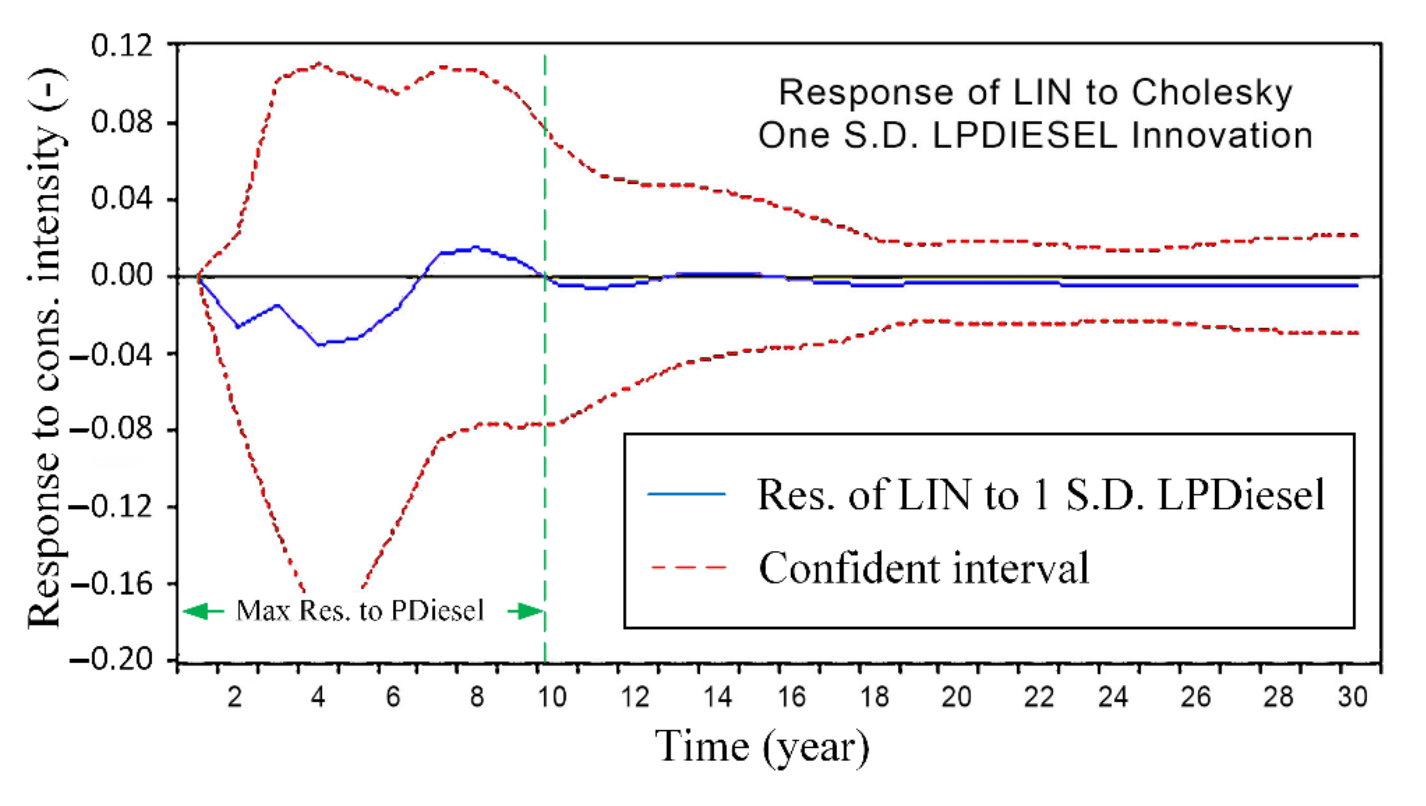
3.5. The Energy Intensity Reaction Due to Shocks in Diesel Energy Price

In Figure 2, the predicted influence of a diesel price impulse on the rate of a standard deviation due to the energy consumption intensity is reported. As presented, if the shocks have occurred an amount of a standard deviation on diesel price, the effects of these shocks will decrease in term seventh. The following period increased and finally has obliterated. Therefore, these shocks have a decreased trend initially and following it increased and finally has been obliterated and has a downturn trend which demonstrated the convergent feature. The maximum response to the diesel price (see the dashed green line) is similarly reported up to the 10th year of the analysis. As presented in Figure 2, the maximum effect is observed in the fourth period by approximately 25%, between 2020 and 2050. Between 4th and 10th years, the reaction fluctuates, gradually decreased. Finally, in the 15th year, it is fully suppressed.

Figure 2. The estimated effect of a diesel price impulse on the rate of a standard deviation due to the energy consumption intensity, between 2020–2050.

Figure 2. The estimated effect of a diesel price impulse on the rate of a standard deviation due to the energy consumption intensity, between 2020–2050.

Figure 3. The estimated effect of a gas price impulse on the rate of a standard deviation due to the energy consumption intensity, between 2020–2050.

Figure 3. The estimated effect of a gas price impulse on the rate of a standard deviation due to the energy consumption intensity, between 2020–2050.

3.6. The Energy Intensity Reaction Due to Shocks in Gas Energy Price

In Figure 3, the estimated effect of a gas price impulse on the rate of a standard deviation due to the energy consumption intensity is presented, for 2020 to 2050. If the shock has occurred an amount of a standard deviation on gas price, the effects of these shocks would increase in term forth, then decrease and finally have obliterated. Therefore, the gas price has been increased, which leads to energy consumption intensity. The maximum response to changes of the gas price is surprisingly decreased to 6th year (see dashed green line) in comparison to the electricity and diesel price changes. As seen in Figure 3, the maximum effect is spotted in the 3rd year by almost 30% and fluctuates until 7th year. Finally, it is settled in the 6th year. Hence, the shocking reaction toward gas price changes has happen earlier than other type of energies discussed (electricity and diesel) in this research.

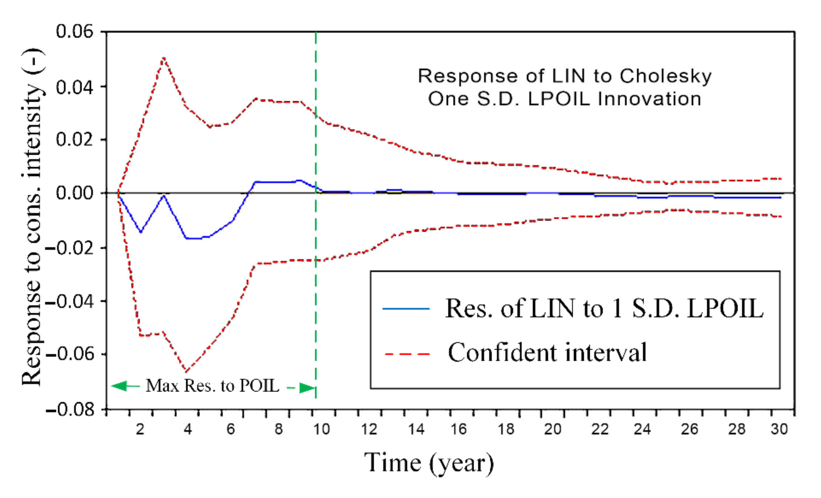
3.7. The Energy Intensity Reaction Due to Shocks in Oil Energy Price

Figure 4 presents the predicted impact of an oil price impulse on the rate of a standard deviation, due to the energy consumption intensity. As shown, if the shock has occurred a considerable amount of the standard deviation on oil price, the effects of this shocks can be decreased in the 6th year. The time-series trend explains that a consequent fluctuation exists between 2nd and 6th years, and finally has obliterated after 10th year. The effects of these shocks increased in term eighth, also represented the converge shocks. The dashed green line indicates the maximum reaction to the oil price change, up to the first 10th year. As given in Figure 4, the maximum effect in the 4th year is approximately 25%, between 2020 to 2050. It should be noted that a similar reaction could be observed in the 2nd year. Meaning that the oil and gas price changes have shown the highest shocks. This considerable shock is gradually decreased, but later neutralized (about 10th year) later than gas. Hence, the shocking reaction of the oil price is somewhat has begun early and ended later than the gas price. This implies the dependency of the economy on oil and gas more than any other type of energies.

Note that all the percentages are based on the reaction rates obtained in this study, see the vertical axis, in Figure 1, Figure 2, Figure 3 and Figure 4. Therefore, the evaluation metrics used the annual historic energy prices and the VAR model’s estimation (output) is unitless, as it is presenting the response rate due to the energy consumption reaction for the next 30 years (2020–2030).

3.8. Estimation of a Long-Term Relationship

After analyzing the effects of institute products on other variables, the long-term relationship has been estimated, and the co-integration equation is computed. In addition, one of the prominent methods to obtain this purpose is Engel-Granger and Johansen-Juselius methods, to provide cointegration vectors in this work.

In this method, the long-term relationship of the studied variables is obtained. The maximum engine value test and trace test have been used to identify the number of cointegrated links. The maximum engine value has tested a null hypothesis which represents not existing relation against existing a co-integrated connection. It is also tested existing one or less than one relation against two existing co-integrated relations. If the test statistics for the studied variables are more than 5%, against the null hypothesis is accepted. Therefore, the number of integrated vectors can be obtained. In the next stage, the cointegrated vector is normalized. In addition, the values based on maximum engine value and trace tests are as follow, (1) without intercept and trend; (2) with restricted intercept and without trend; (3) with unrestricted intercept and without trend; and (4) with unrestricted intercept and with a restricted trend.

Figure 4. The predicted impact of an oil price impulse on the rate of a standard deviation due to the energy consumption intensity, between 2020–2050.

Figure 4. The predicted impact of an oil price impulse on the rate of a standard deviation due to the energy consumption intensity, between 2020–2050.

In this study, the third model is used which is a cointegrated vector by 5%, reported in Table 6. Table 6 and Table 7 present the results obtained by the Johansen co-integration test for both maximum and trace eigenvalue statistics. The maximum value indicates that the null hypothesis of absence of co-integrating relation r = 0 can be rejected at a 5% level of significance. The null hypothesis for r ≤ 1 co-integrating relation can be rejected. Whereas, the null hypothesis of r ≤ 3 cannot be rejected, and the hypothesis against r = 4 is accepted. Since the test statistics are more than critical values. After determining the pattern of vectors stacked next step, a vector stack can stretch the long-term variable on the theory of economic and expected signs to express variables.

4. Normalization of the Co-Integrated Vector

For a better interpretation of the estimation results, the dependent variable coefficient must be, normalized and equal to one. However, the dependent variable coefficient of the Johansen-Juselius method is between 0–0.999, attempting to normalize the real value to 1, to provide its long-term relationship. Hence, all the dependent and the independent variables have been normalized based on the energy consumption intensity coefficient. Table 8 reports the type of relationship that variables have and their effects on the energy intensity. To normalize the estimated coefficients, all the coefficients of the dependent variable and the coefficients of the independent variables (on the predicted coefficient) are divided. In this study, the energy consumption intensity is evaluated. Therefore, the coefficients based on this variable are normalized. The long-term relationship between variables is:

$$\begin{array}{cc}\mathrm{Energy} \mathrm{Intensity}& =0.01\mathrm{GDP}-0.27\mathrm{Capital}+0.61\mathrm{Labor}-0.38\mathrm{Pelectricity}-0.59\mathrm{Pdisesl}-0.78\mathrm{Pgas}\hfill \\ & -0.76\mathrm{Poil}-0.59\hfill \end{array}$$

(28)

based on the relationship shown in Equation (28), the coefficients indicate a negative correlation between capitals and energy prices with energy consumption intensity, while there is a positive relationship between GDP and labor with energy consumption intensity.

Table 6. The results of the cointegrated test based on maximum engine value statistics.

The Number of Convergence Vectors Based on the Null Hypothesis	The Number of Convergence Vectors Based on the against Null Hypothesis	Test Statistics	Critical Value
r = 0	r = 1	229.4940	52.3626
r ≤ 1	r = 2	70.4923	46.2314
r ≤ 2	r = 3	50.3124	40.0775
r ≤ 3	r = 4	31.2800	33.8768
r ≤ 4	r = 5	0.1356	9.1645

Table 6. The results of the cointegrated test based on maximum engine value statistics.

The Number of Convergence Vectors Based on the Null Hypothesis	The Number of Convergence Vectors Based on the against Null Hypothesis	Test Statistics	Critical Value
r = 0	r = 1	229.4940	52.3626
r ≤ 1	r = 2	70.4923	46.2314
r ≤ 2	r = 3	50.3124	40.0775
r ≤ 3	r = 4	31.2800	33.8768
r ≤ 4	r = 5	0.1356	9.1645

Table 7. The results of the cointegrated test based on trace test.

The Number of Convergence Vectors Is Based on the Null Hypothesis	The Number of Convergence Vectors Based on the against Hypothesis	Test Statistics	Critical Value
r = 0	r = 1	428.447	159.520
r ≤ 1	r = 2	198.950	125.610
r ≤ 2	r = 3	128.46	95.750
r ≤ 3	r = 4	78.148	69.810
r ≤ 4	r = 5	46.868	47.856

Table 7. The results of the cointegrated test based on trace test.

The Number of Convergence Vectors Is Based on the Null Hypothesis	The Number of Convergence Vectors Based on the against Hypothesis	Test Statistics	Critical Value
r = 0	r = 1	428.447	159.520
r ≤ 1	r = 2	198.950	125.610
r ≤ 2	r = 3	128.46	95.750
r ≤ 3	r = 4	78.148	69.810
r ≤ 4	r = 5	46.868	47.856

Estimation of Vector Error Correction Model (VECM)

This statistical analysis, carried in this study, has advantaged from the VECM approach, in which the unit root and cointegration tests are conducted through the VECM. This test is employed to verify whether a long-term and stable relationship exists between variables. For examining both the short/long term and causality relationships, the VECM is significantly more powerful among all variables.

The vector error correction model uses the selective convergence vector, which represents the long-term relationship between the variables and estimates their short-term relationship. The coefficient of vector error correction, which is variable-based and normalized indicates the convergence of the model and its defined variables. In the VCEM, the convergence condition is the error correction coefficient, that is statistically notable. The absolute value of the coefficient is between zero and one, and it has also a negative value [42].

In Table 9, the vector error correction is 0.15, and the estimated t-test is −2.8859, indicating its significance. Note that the normalized values are between zero and one in this table. Simultaneous establishment of these three conditions proves the convergence of the variables in the model. Therefore, the studied variables have a long-term relationship.

Table 8. Estimated long-term elasticity using normalized coefficients based on energy intensity.

Intensity	GDP	Capital	Labor	Electricity Price	Diesel Price	Gas Price	Oil Price	c
1	−0.0109	0.2725	−0.6173	0.3803	0.5856	0.7750	0.7643	0.5888

Note that c shows the constant coefficient from the normalization of the coefficients resulted from the VAR model.

Table 8. Estimated long-term elasticity using normalized coefficients based on energy intensity.

Intensity	GDP	Capital	Labor	Electricity Price	Diesel Price	Gas Price	Oil Price	c
1	−0.0109	0.2725	−0.6173	0.3803	0.5856	0.7750	0.7643	0.5888

Note that c shows the constant coefficient from the normalization of the coefficients resulted from the VAR model.

Table 9. Normalized error correction coefficients based on the energy intensity using VECM.

∆ Energy Intensity	∆ GDP	∆ Capital	∆ Labor	∆ Price of Electricity	∆ Price of Diesel	∆ Price of Gas	∆ Price of Oil	VECM
−0.101	−0.753	0.005	0.126	0.101	0.225	0.152	0.165	−0.153
(−0.684)	(−3.597)	(0.558)	(3.352)	(1.482)	(2.572)	(−2.138)	(−2.938)	(−2.885)

Note that the values inside the parenthesis are t-statistics values.

Table 9. Normalized error correction coefficients based on the energy intensity using VECM.

∆ Energy Intensity	∆ GDP	∆ Capital	∆ Labor	∆ Price of Electricity	∆ Price of Diesel	∆ Price of Gas	∆ Price of Oil	VECM
−0.101	−0.753	0.005	0.126	0.101	0.225	0.152	0.165	−0.153
(−0.684)	(−3.597)	(0.558)	(3.352)	(1.482)	(2.572)	(−2.138)	(−2.938)	(−2.885)

Note that the values inside the parenthesis are t-statistics values.

5. Conclusions

5.1. Research Contribution and Findings

The price liberalization has been studied to improve productivity, manage energy consumption, and modify the energy consumption pattern in production enterprises. In this paper, the estimation of liberalization affects—the energy price impacts on energy consumption intensity are investigated. The purpose of the research is modeling and investigating the influence of energy price correction on the energy consumption intensity in the country’s electricity industry.

The historic research data, between 1988 to 2020, is used for modeling purposes. The research method is based on the co-integration model for forecasting the long-run relationship among the studied variables and energy consumption intensity. The VAR model is employed to calculate and analyze the action and reaction functions, in order to investigate the future shocks between 2020 up to 2050, considering a new price shock, in the Iranian energy market for the first time.

The ADF test has analyzed the static data, and shown that all the variables are static at one level. In addition, three criteria such as AIC, SBC, HQC indexes are used to find out the optimal lag number, where the SBC index has performed the best in terms of accuracy. Therefore, the shocks’ effect has been estimated on the price energy, which is studied via a standard deviation on energy consumption intensity with GDP, capital, and labor variables. This result has represented the converge model, which increases the period’s fluctuation and decreases energy consumption intensity. The results have shown that the electricity and oil prices liberalization lead to decreased energy intensity about 25% in the early period after its policy execution. It has also a maximum reduction in consumption in an earlier year. After, it has declined the reduction of energy intensity by 12% in subsequent years, while the oil price effect has experienced an increase of less than 10%. The diesel price effects have reduced the energy intensity by 20% after that has increased by 9%. Whereas, the gas price effects are inverse, and it has resulted in the energy intensity increase by 30%, and decreased gradually in the following years. For all types of energies studied in the paper, estimation’s fluctuations have been observed for some years, mainly in the first 10 years. During the 10th to 15th years, the end-user reaction curve has neutralized because of adapting to the rising energy prices.

Based on the results, the energy price liberalization leads to a decreasing energy consumption intensity in the electricity industry. To forecast the long-term relationships among the pre-defined and economic-focused variables, as a function of the energy intensity coefficient and the price of different energies (electricity, diesel, oil, gas). Finally, the vector error correction coefficient has been calculated by −0.15, and the t-test estimated by −2.8859, which implies that the long-term relationships are meaningful in this work. Hence, the studied variables have long-term relationships and convergent.

5.2. Future Directions

Since the industrial sector has a pivotal place in any country’s economic development, the increase in the energy prices and the elimination of subsidies policy should be imposed gradually, in several stages, to make the necessary reforms and adaptations. It should offer a fast and precise explanation of the experimental test achievements.

Subsides influence the consumer preferences and increase the consumption of subsidized goods. Since the consumer does not pay the accurate price of the goods since they do not consume optimize. If the government interference in the pricing system decreases, the economy’s transparency could be cleared, and the distraction from the productive investment can be decreased. After eliminating the subsidies to these energies, which of course leads to rising energy prices, the industrial sector will face demand and production costs pressure. The sudden increase in energy prices causes the energy-intensive industries in the country to lose the opportunity to invest and restructure to reduce the energy consumption. Therefore, production in the industrial sector will be decreased. With the production reduction due to the elimination of subsidies, the demand of the industries for raw materials will be also reduced. As a result, the need for the raw materials industries will be decreased. In the future studies, the authors are interested to define several policies, in several steps and investigate the impact of each policy on the energy consumption intensity.

5.3. Policy Implications

The suggestion for the policymakers is to provide a suitable environment to create a culture before liberalizing the energy price, however, this is a time-consuming scenario. To adopt to such a change, it takes considerable time (years) for the end-users, and that is why the estimation of the reaction (or shock) analysis for the energy price liberalization is important for the policymakers. The governments need to impose proper regulations, in which the price pressure and reverse influence are considered. It might be better to implement energy rationing for different industries based on the categorical energy consumption. In addition, the government should evaluate the amount of energy consumption and the basis on the amount of consumption for each category of the end-users for a more optimized energy allocation policy. Additionally, it is vital to recognize the industrial firms (or manufacturers) who consumed energy excessively, therefore, the pricing strategy can be enhanced to efficiently influence all kinds of end-users (residential and industrial).

References

1. Nicolli, F.; Vona, F. Energy market liberalization and renewable energy policies in OECD countries. Energy Policy 2019, 128, 853–867. [Google Scholar] [CrossRef] [Green Version]
2. Gajdzik, B.; Sroka, W.; Vveinhardt, J. Energy Intensity of Steel Manufactured Utilising EAF Technology as a Function of Investments Made: The Case of the Steel Industry in Poland. Energies 2021, 14, 5152. [Google Scholar] [CrossRef]
3. Ginevičius, R.; Bilan, Y.; Kądzielawski, G.; Novotny, M.; Kośmider, T. Evaluation of the Sectoral Energy Development Intensity in the Euro Area Countries. Energies 2021, 14, 5298. [Google Scholar] [CrossRef]
4. Energy Ministry of Iran. Energy Balance 1981–2012. Electricity and Energy Macro Planning Office. Available online: www.pep.moe.gov.ir (accessed on 10 June 2021).
5. Jayaprakash, S.; Nagarajan, M.D.; de Prado, R.P.; Subramanian, S.; Divakarachari, P.B. A Systematic Review of Energy Management Strategies for Resource Allocation in the Cloud: Clustering, Optimization and Machine Learning. Energies 2021, 14, 5322. [Google Scholar] [CrossRef]
6. Szymczyk, K.; Şahin, D.; Bağcı, H.; Kaygın, C.Y. The Effect of Energy Usage, Economic Growth, and Financial Development on CO2 Emission Management: An Analysis of OECD Countries with a High Environmental Performance Index. Energies 2021, 14, 4671. [Google Scholar] [CrossRef]
7. Callau-Zori, M.; Samoila, L.; Orgerie, A.-C.; Pierre, G. An experiment-driven energy consumption model for virtual machine management systems. Sustain. Comput. Inform. Syst. 2018, 18, 163–174. [Google Scholar] [CrossRef] [Green Version]
8. Jeong, D.; Park, C.; Ko, Y.M. Short-term electric load forecasting for buildings using logistic mixture vector autoregressive model with curve registration. Appl. Energy 2021, 282, 116249. [Google Scholar] [CrossRef]
9. Li, M.; Zhang, Y. Bootstrapping multivariate portmanteau tests for vector autoregressive models with weak assumptions on errors. Comput. Stat. Data Anal. 2022, 165, 107321. [Google Scholar] [CrossRef]
10. Guefano, S.; Tamba, J.G.; Azong, T.E.W.; Monkam, L. Methodology for forecasting electricity consumption by Grey and Vector autoregressive models. MethodsX 2021, 8, 101296. [Google Scholar] [CrossRef]
11. Bojnec, Š.; Križaj, A. Electricity Markets during the Liberalization: The Case of a European Union Country. Energies 2021, 14, 4317. [Google Scholar] [CrossRef]
12. Topcu, E.; Altinoz, B.; Aslan, A. Global evidence from the link between economic growth, natural resources, energy consumption, and gross capital formation. Resour. Policy 2020, 66, 101622. [Google Scholar] [CrossRef]
13. Rehman, A.; Ma, H.; Ahmad, M.; Ozturk, I.; Işık, C. Estimating the connection of information technology, foreign direct investment, trade, renewable energy and economic progress in Pakistan: Evidence from ARDL approach and cointegrating regression analysis. Energy Econ. 2021, 92, 104937. [Google Scholar]
14. Sheng, X.; Gupta, R.; Ji, Q. The impacts of structural oil shocks on macroeconomic uncertainty: Evidence from a large panel of 45 countries. Energy Econ. 2020, 91, 104940. [Google Scholar] [CrossRef]
15. Zhao, X.-G.; Hu, S.-R. Does market-based electricity price affect China’s energy efficiency? Energy Econ. 2020, 91, 104909. [Google Scholar]
16. Norouzi, N.; Bashashjafarabadi, Z.; Meybodi, S.M.Y. An Economic Evaluation of the Use of Wind Farms in Iran, Taking into Account the Effect of Energy Price Liberalization Policy. Univers. J. Bus. Manag. 2021, 1, 49–61. [Google Scholar]
17. Salmanzadeh-Meydani, N.; Ghomi, S.M.T.F. The causal relationship among electricity consumption, economic growth and capital stock in Iran. J. Policy Modeling 2019, 41, 1230–1256. [Google Scholar] [CrossRef]
18. Oryani, B.; Koo, Y.; Rezania, S. Structural Vector Autoregressive Approach to Evaluate the Impact of Electricity Generation Mix on Economic Growth and CO2 Emissions in Iran. Energies 2020, 13, 4268. [Google Scholar] [CrossRef]
19. Pezzutto, S.; Grilli, G.; Zambotti, S.; Dunjic, S. Forecasting Electricity Market Price for End Users in EU28 until 2020—Main Factors of Influence. Energies 2018, 11, 1460. [Google Scholar] [CrossRef] [Green Version]
20. Pan, X.; Uddin, M.K.; Saima, U.; Jiao, Z.; Han, C. How to do industrialization and trade openness influence energy intensity? Evidence from a path model in case of Bangladesh. Energy Policy 2019, 133, 110916. [Google Scholar] [CrossRef]
21. Szőke, T.; Hortay, O.; Farkas, R. Price regulation and supplier margins in the Hungarian electricity markets. Energy Econ. 2021, 94, 105098. [Google Scholar] [CrossRef]
22. Gujarati, D.N. Basic Econometrics, 4th ed.; McGrowHill: New York, NY, USA, 2003; pp. 1–1027. ISBN 0-07-112342-3. [Google Scholar]
23. Sims, C.A.; Stock, J.H.; Watson, M.W. Inference in Linear Time Series Models with Some Unit Roots. Econometrica 1990, 56, 113–144. [Google Scholar] [CrossRef]
24. Li, W.; Liao, J. A comparative study on trend forecasting approach for stock price time series. In Proceedings of the 2017 11th IEEE International Conference on Anti-Counterfeiting, Security, and Identification (ASID), Xiamen, China, 27–29 October 2017; pp. 74–78. [Google Scholar]
25. Caporale, G.M.; Gil-Alaña, L.A. Fractional cointegration and tests of present value models. Rev. Financ. Econ. 2004, 13, 245–258. [Google Scholar] [CrossRef] [Green Version]
26. Stock, J.H.; Watson, M.W. Vector Autoregressions. J. Econ. Perspect. 2001, 15, 101–115. [Google Scholar] [CrossRef] [Green Version]
27. Watson, M.W. Vector Autoregressions and Cointegration. In Handbook of Econometrics; Engle, R., McFadden, D., Eds.; Elsevier Science Ltd.: Amsterdam, The Netherlands, 1994; Volume IV, pp. 2844–2915. [Google Scholar]
28. Bakhsh, S.S.; Khansari, Z.H. Application of Eviews in Econometrics; Institute of Economic Affairs: Tehran, Iran, 2005. [Google Scholar]
29. Carta, S.; Medda, A.; Pili, A.; Reforgiato Recupero, D.; Saia, R. Forecasting E-Commerce Products Prices by Combining an Autoregressive Integrated Moving Average (ARIMA) Model and Google Trends Data. Future Internet 2018, 11, 5. [Google Scholar] [CrossRef] [Green Version]
30. Engle, R.F.; Yoo, B.S. Cointegrated Economic Time Series: An Overview with New Results. In Long-Run Economic Relationships: Readings in Cointegration; Engle, R.F., Granger, C.W.J., Eds.; Oxford University Press: Oxford, UK, 1991; pp. 1–301. [Google Scholar]
31. Engle, R.F.; Granger, C.W.J. Cointegration and Error Correction: Representation, Estimation and Testing. Econometrica 1987, 55, 251–276. [Google Scholar] [CrossRef]
32. Johansen, S. Estimation and Hypothesis Testing of Cointegration Vectors in Gaussian Vector Autoregressive Models. Econometrica 1991, 55, 1551–1580. [Google Scholar] [CrossRef]
33. Abbasi, F.; Riaz, K. CO2 emissions and financial development in an emerging economy: An augmented VAR approach. Energy Policy 2016, 90, 102–114. [Google Scholar] [CrossRef]
34. Cavanaugh, J.E. Unifying the Derivations for the Akaike and Corrected Akaike Information Criteria. Stat. Probab. Lett. 2000, 33, 201–208. [Google Scholar] [CrossRef]
35. Snipes, M.; Taylor, D.C. Model selection and Akaike Information Criteria: An example from wine ratings and prices. Wine Econ. Policy 2014, 3, 3–9. [Google Scholar] [CrossRef] [Green Version]
36. Rossi, R.; Murari, A.; Gaudio, P.; Gelfusa, M. Upgrading Model Selection Criteria with Goodness of Fit Tests for Practical Applications. Entropy 2020, 22, 447. [Google Scholar] [CrossRef] [Green Version]
37. Maïnassara, Y.B.; Kokonendji, C.C. Modified Schwarz and Hannan-Quinn information criteria for weak VARMA model. Stat. Inference Stoch. Process. 2016, 19, 199–217. [Google Scholar] [CrossRef]
38. Hall, R.A.; Inoue, A.; Nason, J.M.; Rossi, B. Information criteria for impulse response function matching estimation of DSGE models. Econometrics 2012, 170, 499–518. [Google Scholar] [CrossRef] [Green Version]
39. Virginia, E.; Ginting, J.; Elfaki, F.A.M. Application of GARCH Model to Forecast Data and Volatility of Share Price of Energy (Study on Adaro Energy Tbk, LQ45). Int. J. Energy Econ. Policy 2018, 8, 131–140. [Google Scholar]
40. Ariyo, A.A.; Adewumi, A.O.; Ayo, C.K. Stock Price Prediction Using the ARIMA Model. In Proceedings of the 2014 UKSim-AMSS 16th International Conference on Computer Modelling and Simulation, Cambridge, UK, 26–28 March 2014; pp. 106–112. [Google Scholar]
41. Zhou, M.; Yan, Z.; Ni, Y.; Li, G. An ARIMA approach to forecasting electricity price with accuracy improvement by predicted errors. In Proceedings of the IEEE Power Engineering Society General Meeting, Denver, CO, USA, 6–10 June 2004; Volume 2, pp. 233–238. [Google Scholar]
42. Ky, D.X.; Tuyen, L.T. A Higher Order Markov Model for Time Series Forecasting. Int. J. Appl. Math. Stat. 2018, 57, 1–18. [Google Scholar]
43. Central Bank of the Islamic Republic of Iran. Available online: https://tsd.cbi.ir/Display/Content.aspx (accessed on 10 June 2021).
44. Iran Statistics Center. Available online: https://www.amar.org.ir (accessed on 10 June 2021).
Publisher’s Note: MDPI stays neutral with regard to jurisdictional claims in published maps and institutional affiliations.