
A New Methodological Approach for the Evaluation of Scaling Up a Latent Storage Module for Integration in Heat Pumps

 ,
,  ,
,  ,
,  ,
,  ,
,  and
and 
Abstract
:1. Introduction
2. Materials and Methods
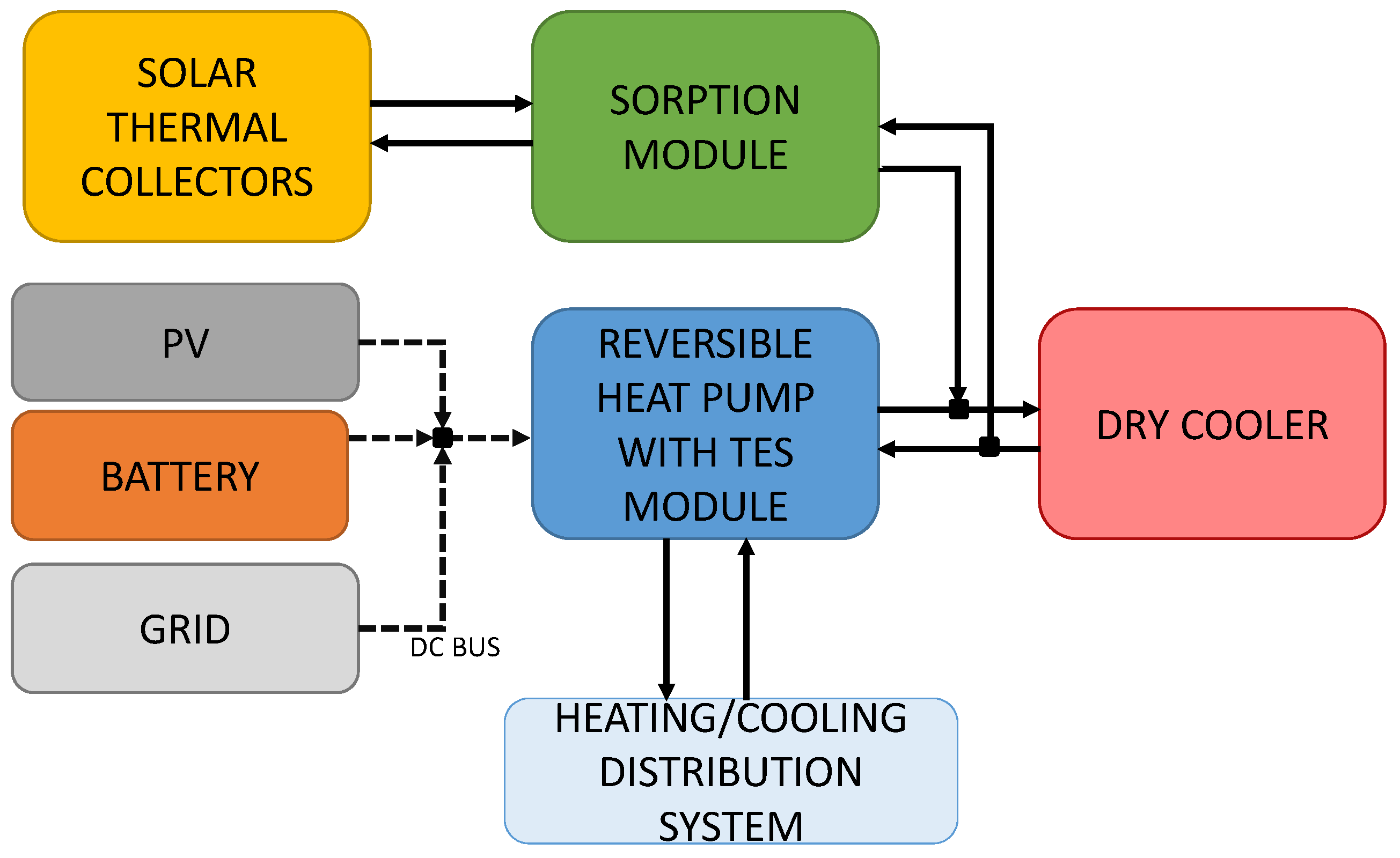
2.1. Description of the Application
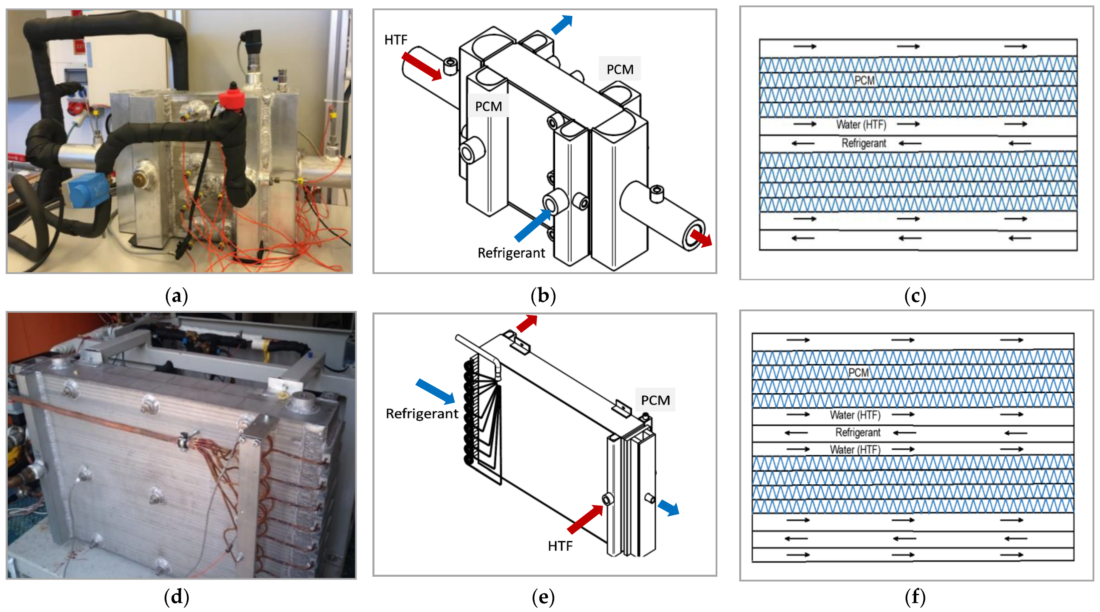
2.2. Description of the Three-Fluids Latent Storage Module
2.3. Description of the Experimental Set-Ups
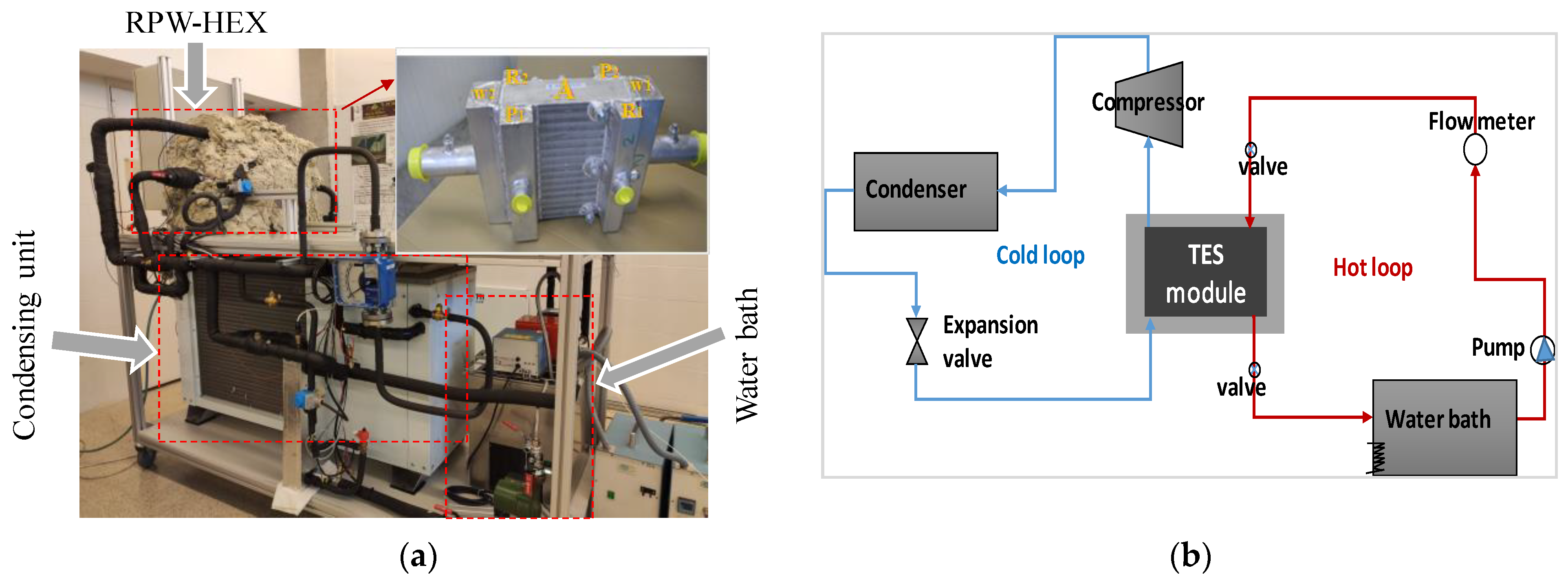
2.3.1. Lab-Scale Testing Set-Up
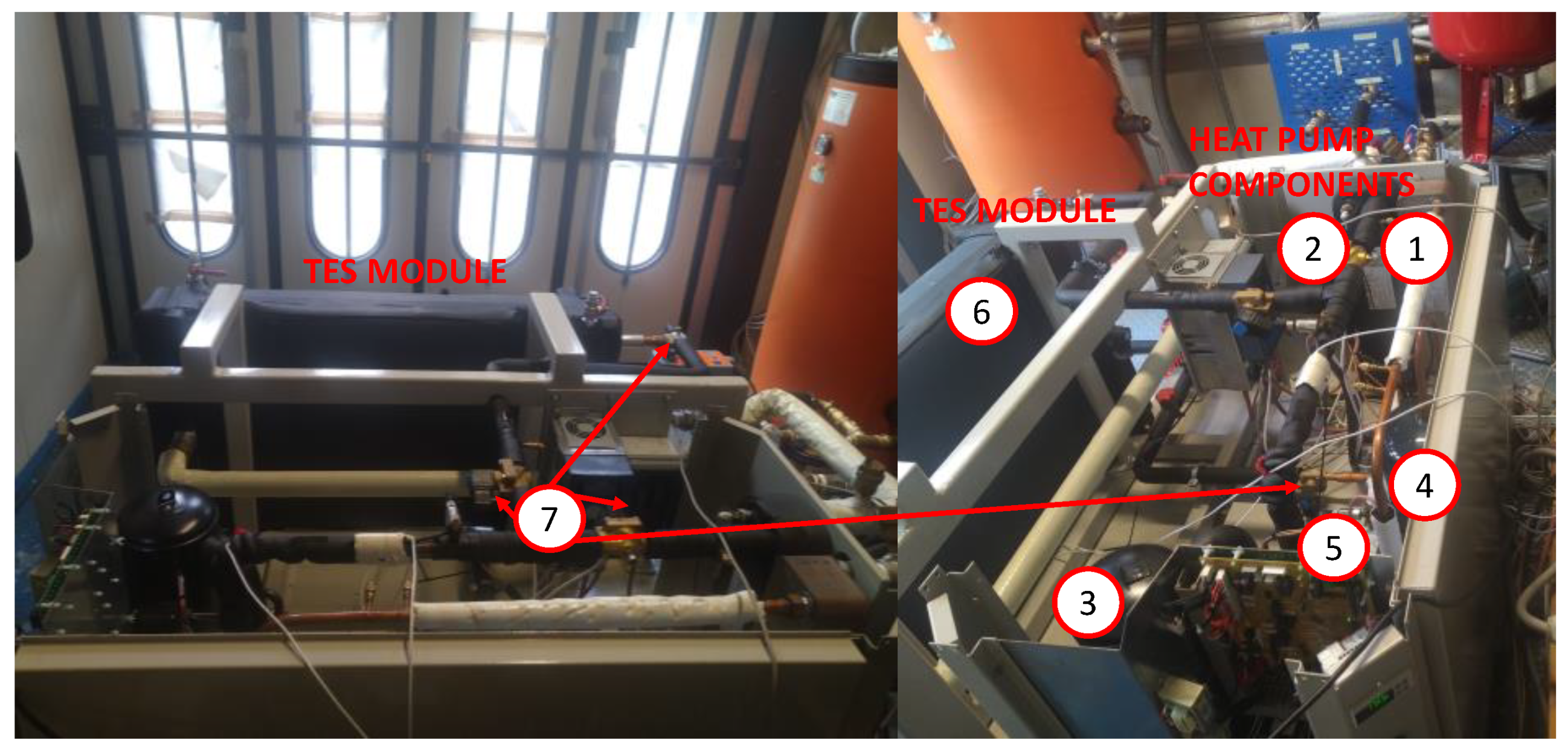
2.3.2. Full-Scale Testing Set-Up
2.4. Materials Properties
2.5. Experimental Methodology
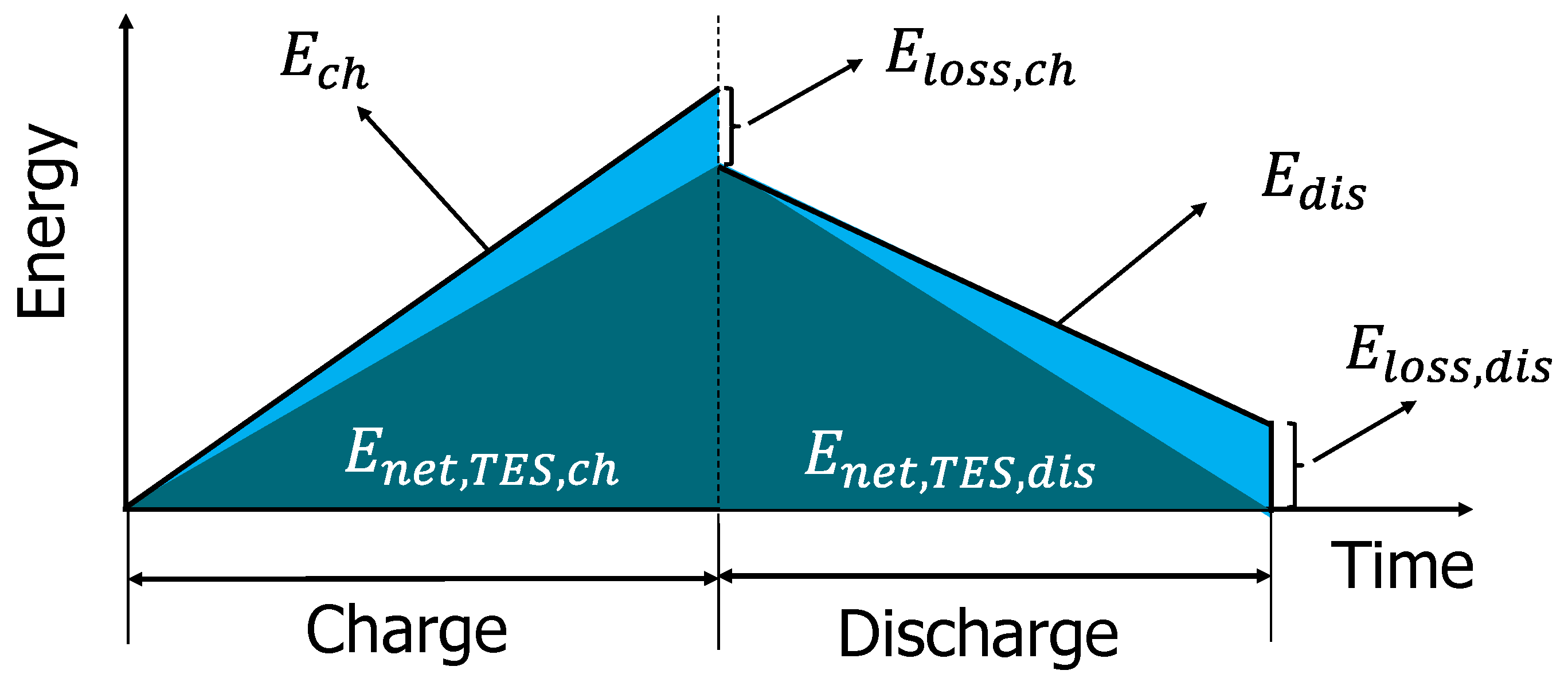
2.6. Theoretical Evaluation
2.7. Definition of the Performance Indicators (PIs) Considered
3. Results
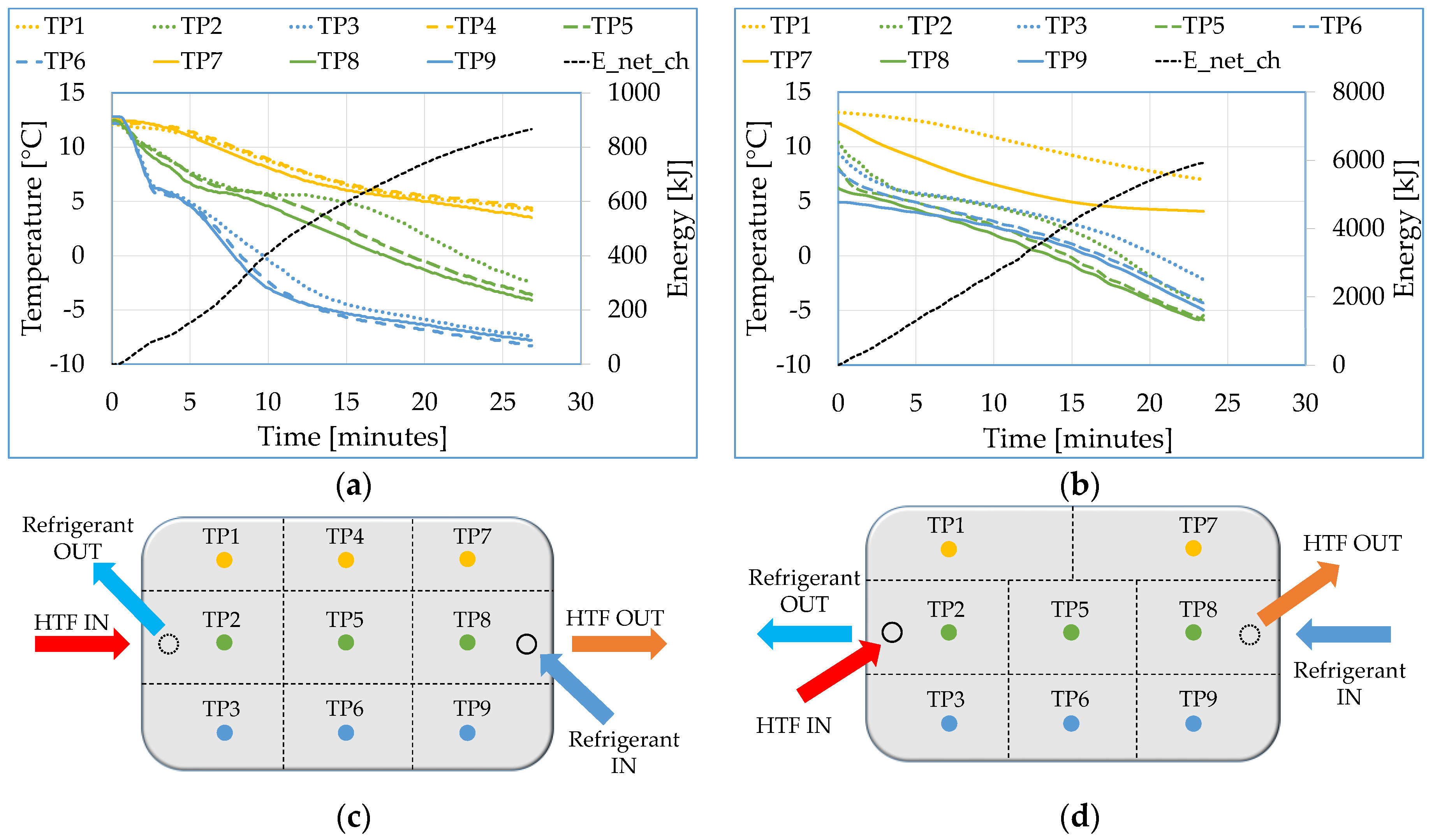
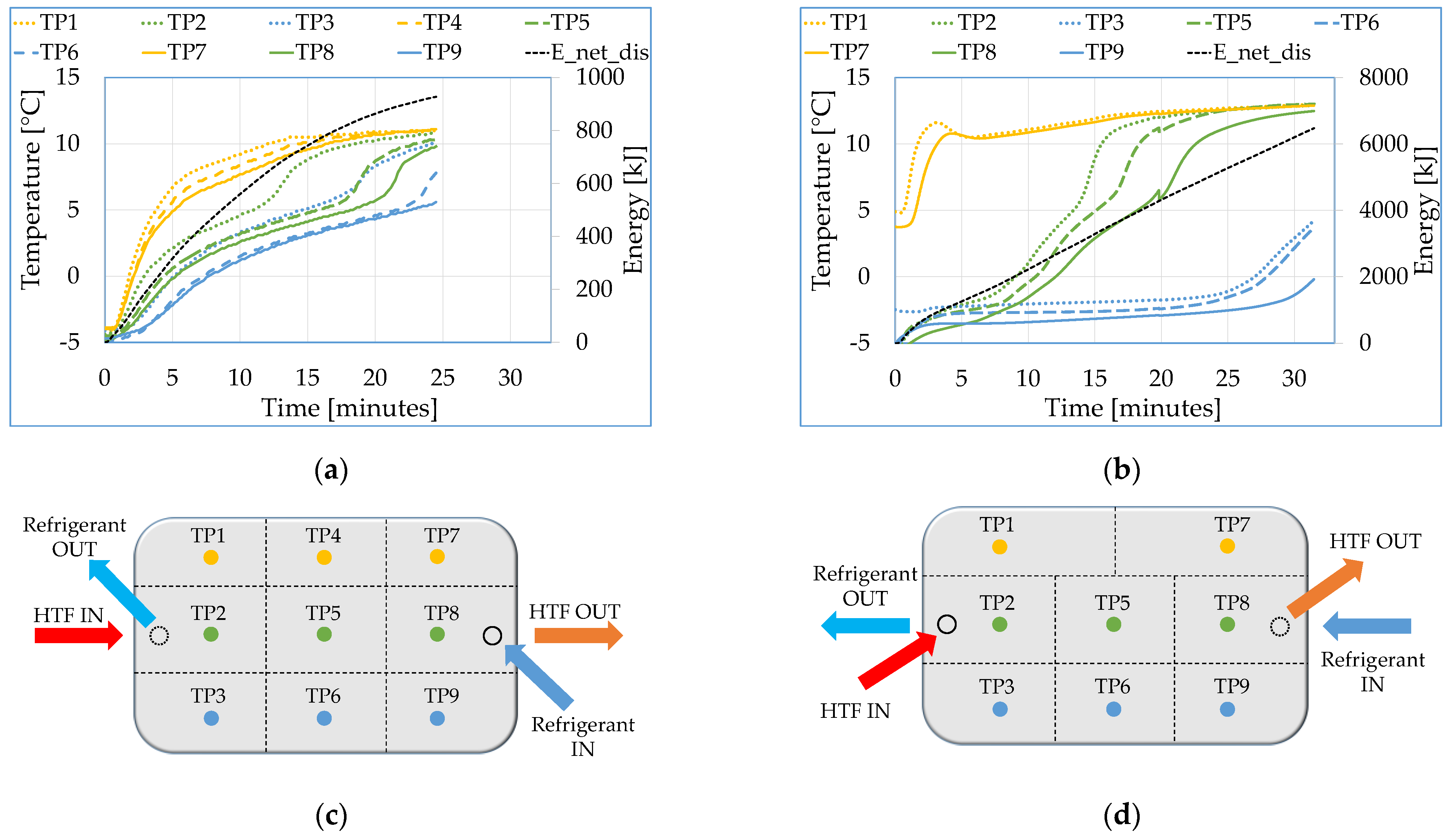
3.1. Test Results
3.2. Results of Calculated PIs
4. Discussion
5. Conclusions
- -
- Different normalization methods can be applied to some of the PIs, depending on the focus of the study and the intended application, which may even lead to discrepant results. When a mass normalization method is used, an improvement in the PCM mass, energy storage capacity, and average charging power is observed, while the average discharging power decreases.
- -
- When a volume normalization method is used, PCM volume, energy storage capacity, and average charging and discharging power increase, especially PCM volume, and energy storage capacity.
- -
- When normalization by surface area of heat transfer is used, no significant changes are obtained in terms of PCM volume and TES capacity of the modules. However, both average charging and discharging power decrease.
- -
- A slight reduction in the energy performance in charge and discharge is observed.
- -
- No significant influence of the scaling up is observed on the charging, discharging, and overall efficiencies.
Author Contributions
Funding
Institutional Review Board Statement
Informed Consent Statement
Data Availability Statement
Acknowledgments
Conflicts of Interest
References
- European Commission. EU 2030 Climate & Energy Framework; European Commission: Brussels, Belgium, 2014. [Google Scholar]
- European Commission. Strategic Energy Technology Plan Implementation Plan; European Commission: Brussels, Belgium, 2018. [Google Scholar]
- Tejero-González, A.; Andrés-Chicote, M.; García-Ibáñez, P.; Velasco-Gómez, E.; Rey-Martínez, F.J. Assessing the applicability of passive cooling and heating techniques through climate factors: An overview. Renew. Sustain. Energy Rev. 2016, 65, 727–742. [Google Scholar] [CrossRef] [Green Version]
- Gullbrekken, L.; Grynning, S.; Gaarder, J.; Gullbrekken, L.; Grynning, S.; Gaarder, J.E. Thermal performance of insulated constructions—Experimental studies. Buildings 2019, 9, 49. [Google Scholar] [CrossRef] [Green Version]
- Fernandez-Antolin, M.-M.; Del Río, J.M.; Costanzo, V.; Nocera, F.; Gonzalez-Lezcano, R.-A. Passive design strategies for residential buildings in different spanish climate zones. Sustainability 2019, 11, 4816. [Google Scholar] [CrossRef] [Green Version]
- Palomba, V.; Borri, E.; Charalampidis, A.; Frazzica, A.; Cabeza, L.F.; Karellas, S. Implementation of a solar-biomass system for multi-family houses: Towards 100% renewable energy utilization. Renew. Energy 2020, 166, 190–209. [Google Scholar] [CrossRef]
- Palomba, V.; Borri, E.; Charalampidis, A.; Frazzica, A.; Karellas, S.; Cabeza, L.F. An innovative solar-biomass energy system to increase the share of renewables in office buildings. Energies 2021, 14, 914. [Google Scholar] [CrossRef]
- Stalinski, D.; Duquette, J. Development of a simplified method for optimally sizing hot water storage tanks subject to short-term intermittent charge/discharge cycles. J. Energy Storage 2021, 37, 102463. [Google Scholar] [CrossRef]
- Singh, R.V.P.; Singh, J.; Mathur, J.; Bhandari, M. Calibrated simulation study for efficient sizing and operating strategies for the thermal storage integrated air conditioning system. Int. J. Sustain. Energy 2021, 40, 389–411. [Google Scholar] [CrossRef]
- Pandey, B.; Banerjee, R.; Sharma, A. Coupled EnergyPlus and CFD analysis of PCM for thermal management of buildings. Energy Build. 2021, 231, 110598. [Google Scholar] [CrossRef]
- Barone, G.; Buonomano, A.; Forzano, C.; Palombo, A. A novel dynamic simulation model for the thermo-economic analysis and optimisation of district heating systems. Energy Convers. Manag. 2020, 220, 113052. [Google Scholar] [CrossRef]
- Emhofer, J.; Marx, K.; Barz, T.; Hochwallner, F.; Cabeza, L.F.; Zsembinszki, G.; Strehlow, A.; Nitsch, B.; Wiesflecker, M.; Pink, W. Techno-economic analysis of a heat pump cycle including a three-media refrigerant/phase change material/water heat exchanger in the hot superheated section for efficient domestic hot water generation. Appl. Sci. 2020, 10, 7873. [Google Scholar] [CrossRef]
- Arabkoohsar, A.; Behzadi, A.; Alsagri, A.S. Techno-economic analysis and multi-objective optimization of a novel solar-based building energy system; An effort to reach the true meaning of zero-energy buildings. Energy Convers. Manag. 2021, 232, 113858. [Google Scholar] [CrossRef]
- Barone, G.; Buonomano, A.; Forzano, C.; Palombo, A.; Panagopoulos, O. Experimentation, modelling and applications of a novel low-cost air-based photovoltaic thermal collector prototype. Energy Convers. Manag. 2019, 195, 1079–1097. [Google Scholar] [CrossRef]
- Hulteberg, C.; Leveau, A. Scaling up a gas-phase process for converting glycerol to propane. Catalysts 2020, 10, 1007. [Google Scholar] [CrossRef]
- Della Torre, A.; Montenegro, G.; Onorati, A.; Khadilkar, S.; Icarelli, R. Multi-scale CFD modeling of plate heat exchangers including offset-strip fins and dimple-type turbulators for automotive applications. Energies 2019, 12, 2965. [Google Scholar] [CrossRef] [Green Version]
- Prieto, C.; Osuna, R.; Fernández, A.I.; Cabeza, L.F. Molten salt facilities, lessons learnt at pilot plant scale to guarantee commercial plants; heat losses evaluation and correction. Renew. Energy 2016, 94, 175–185. [Google Scholar] [CrossRef] [Green Version]
- Touzo, A.; Olives, R.; Dejean, G.; Pham Minh, D.; El Hafi, M.; Hoffmann, J.F.; Py, X. Experimental and numerical analysis of a packed-bed thermal energy storage system designed to recover high temperature waste heat: An industrial scale up. J. Energy Storage 2020, 32, 101894. [Google Scholar] [CrossRef]
- Patil, R.S.; Pandey, M.; Mahanta, P. Parametric studies and effect of scale-up on wall-to-bed heat transfer characteristics of circulating fluidized bed risers. Exp. Therm. Fluid Sci. 2011, 35, 485–494. [Google Scholar] [CrossRef]
- Godoy, V.A.; Zuquette, L.V.; Gómez-Hernández, J.J. Scale effect on hydraulic conductivity and solute transport: Small and large-scale laboratory experiments and field experiments. Eng. Geol. 2018, 243, 196–205. [Google Scholar] [CrossRef]
- Wang, X.Y.; Spearpoint, M.J.; Fleischmann, C.M. Comparison of results from large-scale and small-scale tunnel experiments. Fire Saf. J. 2018, 95, 135–144. [Google Scholar] [CrossRef]
- Sun, X.; Hu, L.; Zhang, X.; Yang, Y.; Ren, F.; Fang, X.; Wang, K.; Lu, H. Temperature evolution and external flame height through the opening of fire compartment: Scale effect on heat/mass transfer and revisited models. Int. J. Therm. Sci. 2021, 164, 106849. [Google Scholar] [CrossRef]
- Frankovič, A.; Ducman, V.; Dolenec, S.; Panizza, M.; Tamburini, S.; Natali, M.; Pappa, M.; Tsoutis, C.; Bernardi, A. Up-scaling and performance assessment of façade panels produced from construction and demolition waste using alkali activation technology. Constr. Build. Mater. 2020, 262, 120475. [Google Scholar] [CrossRef]
- HYBUILD. Available online: http://www.hybuild.eu/ (accessed on 4 December 2020).
- Palomba, V.; Bonanno, A.; Brunaccini, G.; Aloisio, D.; Sergi, F.; Dino, G.E.; Varvaggiannis, E.; Karellas, S.; Nitsch, B.; Strehlow, A.; et al. Hybrid cascade heat pump and thermal-electric energy storage system for residential buildings: Experimental testing and performance analysis. Energies 2021, 14, 2580. [Google Scholar] [CrossRef]
- Mselle, B.D.; Vérez, D.; Zsembinszki, G.; Borri, E.; Cabeza, L.F. Performance study of direct integration of phase change material into an innovative evaporator of a simple vapour compression system. Appl. Sci. 2020, 10, 4649. [Google Scholar] [CrossRef]
- Brancato, V.; Gordeeva, L.G.; Sapienza, A.; Palomba, V.; Vasta, S.; Grekova, A.D.; Frazzica, A.; Aristov, Y.I. Experimental characterization of the LiCl/vermiculite composite for sorption heat storage applications. Int. J. Refrig. 2018, 105, 92–100. [Google Scholar] [CrossRef]
- Rubitherm RT-PCM. Available online: https://www.rubitherm.eu/en/index.php/productcategory/organische-pcm-rt (accessed on 2 October 2019).
- Mselle, B.D.; Zsembinszki, G.; Vérez, D.; Borri, E.; Cabeza, L.F. A detailed energy analysis of a novel evaporator with latent thermal energy storage ability. Appl. Therm. Eng. 2021, in press. [Google Scholar]
- Carvill, J. Thermodynamics and heat transfer. Mech. Eng. Data Handb. 1993, 102–145. [Google Scholar] [CrossRef]
- IT, R. Rockwool Data Sheet. Available online: https://www.rockwool.com/north-america/resources-and-tools/documentation/ (accessed on 2 October 2019).
- ISOVER Saint-Gobain Data Sheet TECH Wired Mat MT 3.1. Available online: https://www.isover.es/productos/tech-wired-mat-mt-31 (accessed on 2 October 2019).
- Palomba, V.; Frazzica, A. A fast-reduced model for an innovative latent thermal energy storage for direct integration in heat pumps. Appl. Sci. 2021, 11, 8972. [Google Scholar] [CrossRef]
- Palomba, V.; Frazzica, A.; Gasia, J.; Cabeza, L.F. Experimental characterization of latent thermal energy storage systems. In Recent Advancements in Materials and Systems for Thermal Energy Storage—An Introduction to Experimental Characterization Methods; Frazzica, A., Cabeza, L.F., Eds.; Springer: Berlin/Heidelberg, Germany, 2019; pp. 173–200. ISBN 978-3-319-96640-3. [Google Scholar]
- Palomba, V.; Gasia, J.; Romaní, J.; Frazzica, A.; Cabeza, L.F. Definition of performance indicators for thermal energy storage. In Recent Advancements in Materials and Systems for Thermal Energy Storage—An Introduction to Experimental Characterization Methods; Frazzica, A., Cabeza, L.F., Eds.; Springer: Berlin/Heidelberg, Germany, 2019; pp. 227–242. ISBN 978-3-319-96640-3. [Google Scholar]


| Variable | Lab-Scale | Full-Scale |
|---|---|---|
| Number of PCM layers (-) | 24 | 44 |
| Number of refrigerant channels (-) | 5 | 10 |
| Number of HTF channels (-) | 7 | 22 |
| Module height (m) | 0.310 | 0.637 |
| Module length (m) | 0.420 | 1.100 |
| Module width (m) | 0.094 | 0.160 |
| Mass of PCM (kg) | 3.7 | 40.0 |
| Mass of aluminum (kg) | 20.4 | 148.0 |
| Mass of HTF inside the module (kg) | 3.3 | 5.0 |
| Total mass without insulation (kg) | 27.4 | 193.0 |
| Mass of insulation (kg) | 6.9 | 23.0 |
| Total mass including insulation (kg) | 34.3 | 216.0 |
| Volume without insulation (m3) | 0.0153 | 0.1166 |
| Volume including insulation (m3) | 0.1210 | 0.4701 |
| Heat transfer area of PCM layers (m2) | 0.34 | 3.52 |
| Process | Lab-Scale | Full-Scale |
|---|---|---|
| Charge | Cooling fraction (%) | Compressor frequency (Hz) |
| 20 | 25 | |
| Discharge | HTF flow rate (L·h−1) | HTF flow rate (L·h−1) |
| 100 | 900 |
| Performance Indicator (PI) | Normalization | Symbol | Units | Lab-Scale | Full-Scale | Variation |
|---|---|---|---|---|---|---|
| PCM mass | mass | kg·kg−1 | 0.11 | 0.19 | 73% | |
| PCM volume | volume | m3·m−3 | 0.04 | 0.11 | 178% | |
| area | m3·m−2 | 0.014 | 0.015 | 4% | ||
| Energy storage capacity | mass | kJ·kg−1 | 22.6 | 34.4 | 52% | |
| volume | MJ·m−3 | 6.4 | 15.6 | 145% | ||
| area | MJ·m−2 | 2.27 | 2.09 | −8% | ||
| Charging power | mass | W·kg−1 | 16.3 | 19.7 | 21% | |
| volume | kW·m−3 | 4.6 | 9.0 | 94% | ||
| area | kW·m−2 | 1.6 | 1.2 | −27% | ||
| Discharging power | mass | W·kg−1 | 18.7 | 15.8 | −16% | |
| volume | kW·m−3 | 5.3 | 7.2 | 36% | ||
| area | kW·m−2 | 1.9 | 1.0 | −49% | ||
| Charging performance | - | - | 0.97 | 0.81 | −17% | |
| Discharging performance | - | - | 0.99 | 0.85 | −15% | |
| Charging efficiency | - | - | 0.97 | 0.97 | 0% | |
| Discharging efficiency | - | - | 0.98 | 0.96 | −1% | |
| Overall efficiency | - | - | 0.94 | 0.94 | −1% |
| PI | Normalization Method | |||
|---|---|---|---|---|
| Mass | Volume | Surface Area | None | |
| PCM mass | ↑↑ | × | × | × |
| PCM volume | × | ↑↑↑ | ≈ | × |
| Energy storage capacity | ↑↑ | ↑↑↑ | ≈ | × |
| Charging power | ↑ | ↑↑ | ↓ | × |
| Discharging power | ↓ | ↑ | ↓↓ | × |
| Charging performance | × | × | × | ↓ |
| Discharging performance | × | × | × | ↓ |
| Charging efficiency | × | × | × | ≈ |
| Discharging efficiency | × | × | × | ≈ |
| Overall efficiency | × | × | × | ≈ |
Publisher’s Note: MDPI stays neutral with regard to jurisdictional claims in published maps and institutional affiliations. |
© 2021 by the authors. Licensee MDPI, Basel, Switzerland. This article is an open access article distributed under the terms and conditions of the Creative Commons Attribution (CC BY) license (https://creativecommons.org/licenses/by/4.0/).
Share and Cite
Zsembinszki, G.; Mselle, B.D.; Vérez, D.; Borri, E.; Strehlow, A.; Nitsch, B.; Frazzica, A.; Palomba, V.; Cabeza, L.F. A New Methodological Approach for the Evaluation of Scaling Up a Latent Storage Module for Integration in Heat Pumps. Energies 2021, 14, 7470. https://doi.org/10.3390/en14227470
Zsembinszki G, Mselle BD, Vérez D, Borri E, Strehlow A, Nitsch B, Frazzica A, Palomba V, Cabeza LF. A New Methodological Approach for the Evaluation of Scaling Up a Latent Storage Module for Integration in Heat Pumps. Energies. 2021; 14(22):7470. https://doi.org/10.3390/en14227470
Chicago/Turabian StyleZsembinszki, Gabriel, Boniface Dominick Mselle, David Vérez, Emiliano Borri, Andreas Strehlow, Birgo Nitsch, Andrea Frazzica, Valeria Palomba, and Luisa F. Cabeza. 2021. "A New Methodological Approach for the Evaluation of Scaling Up a Latent Storage Module for Integration in Heat Pumps" Energies 14, no. 22: 7470. https://doi.org/10.3390/en14227470
APA StyleZsembinszki, G., Mselle, B. D., Vérez, D., Borri, E., Strehlow, A., Nitsch, B., Frazzica, A., Palomba, V., & Cabeza, L. F. (2021). A New Methodological Approach for the Evaluation of Scaling Up a Latent Storage Module for Integration in Heat Pumps. Energies, 14(22), 7470. https://doi.org/10.3390/en14227470