Day-Ahead Forecasting of the Percentage of Renewables Based on Time-Series Statistical Methods

Abstract

Forecasting renewable energy sources is of critical importance to several practical applications in the energy field. However, due to the inherent volatile nature of these energy sources, doing so remains challenging. Numerous time-series methods have been explored in literature, which consider only one specific type of renewables (e.g., solar or wind), and are suited to small-scale (micro-level) deployments. In this paper, the different types of renewable energy sources are reflected, which are distributed at a national level (macro-level). To generate accurate predictions, a methodology is proposed, which consists of two main phases. In the first phase, the most relevant variables having impact on the generation of the renewables are identified using correlation analysis. The second phase consists of (1) estimating model parameters, (2) optimising and reducing the number of generated models, and (3) selecting the best model for the method under study. To this end, the three most-relevant time-series auto-regression based methods of SARIMAX, SARIMA, and ARIMAX are considered. After deriving the best model for each method, then a comparison is carried out between them by taking into account different months of the year. The evaluation results illustrate that our forecasts have mean absolute error rates between 6.76 and 11.57%, while considering both inter- and intra-day scenarios. The best models are implemented in an open-source REN4Kast software platform.

1. Introduction

1.1. Motivation

The increasing integration of renewable energy sources (RES) leads to a more sustainable and cleaner future. Despite the perceptible advantages with respect to the environment, the integration of those RES into the power system should be realised with care. Renewables are intermittent in nature, and their volatility could lead to an imbalance between power generation and demand, which endangers the stability of the grid [1]. To circumvent this situation, there was a paradigm change from traditional “supply follows demand” to “demand-side management” (DSM) [2]. In this regard, the key aspect of DSM is to carry out short-term (e.g., day-ahead) planning and scheduling (e.g., when and how much power to feed-in from renewables or increase/decrease the demand) of the power system. Consequently, this necessitates short-term forecasts of both power generation and demand. In this paper, we focus on generating short-term forecasts for renewables, due to thevlack of contributions in this respect on the one hand, and on the other forecasts for demand have been extensively and exhaustively studied in the literature [3,4,5,6,7,8] (Some of the recent publications).

Generally, there are two different groups which require forecasts for renewables: energy market participants, and power system operators. The former deals with daily business activities such as the buying or selling of energy, whereas the latter is concerned with maintaining the stability of the power system [9,10]. However, both require timely and accurate forecasts of power generation from RES [11,12,13].

Basically, forecasting can be categorised into two groups: physical and statistical models. The former generates forecasts based on the laws of physics (e.g., numerical weather prediction [14], or power demand of processors [15,16]), whereas the latter deals with developing predictions based on historical data [17]. Due to the complexity in generating physical models, usually statistical ones are more favorable when deriving forecasts. Moreover, statistical models can be further decomposed into structural and time-series approaches. The former generates forecasts of the endogenous variable based on one or more exogenous variables (e.g., linear-regression), whereas the latter uses the previous values of the endogenous variable to forecast the future. The advantage of time-series forecasts is that patterns and trends can be captured [18], which is an important requirement when generating forecasts for RES.

1.2. Problem Statement and Research Questions

Time-series forecasting, which is the adopted method in this paper, has fundamental importance to various practical applications in the energy field [19]. Traditionally, it has been tackled using conventional methods, such as exponential smoothing, smoothing techniques, statistical analysis, and regression-based approaches [20]. Among those, auto-regressive and moving average-based methods such as SARIMAX, SARIMA, and ARIMAX [21] received considerable attention, owing to their ability to identify seasonality as well as the impact of exogenous variables on the endogenous one. In the literature, the three above-mentioned methods were used to generate time-series forecasts for the RES. However, those contributions tackle only a single type of renewable sources: either solar or wind energy. Furthermore, the proposed approaches consider a small-scale regional deployment (e.g., solar farms) [22,23,24,25] of RES.

The problem considered in this paper is to generate time-series forecasts for renewable energy sources, which are distributed at a national level (e.g., large-scale). As a matter of fact, unlike the state-of-the-art contributions, which take into account only one type of renewable at small-scale deployments, our goal is to generate forecasts by incorporating different types of renewable energy sources at a large-scale deployment (e.g., nation). Hence, the stated problem reveals the need for a holistic solution. As a contribution to the body of research, the most relevant renewable energy sources of wind, hydro, solar, etc., are considered. Some of the key research questions are:

• Given the fact that power generation from renewables are dependent on weather conditions, what is the minimum number of meteorology-related variables that are required to forecast the generation from different types of renewables?
• Among the three considered time-series regression-based methods, which one is more suitable and under what seasonal conditions?

In order to give answers to the above-mentioned research questions, a methodology consisting of two main phases is proposed, where each such phase comprises of several steps. The main objective of this methodology is to derive the best model for each of the three methods under study, while considering different months of the year. The accuracy of those models are validated by regarding different performance metrics, where each such metric demonstrates a specific characteristic of the derived model. It is important to mention that the need for forecasts of the renewables was first initiated in this paper within the practical application use case of electric-mobility (https://electrific.eu/ accessed on 5 November 2021) [9,10,26,27]. To this end, the electric vehicle (EV) drivers while planning their trip from source to destination have three options to choose from: the fastest, greenest, or cheapest routes. The greenest option requires the EV driver to charge his/her EV at charging stations which are supplied with renewable energy sources. Consequently, in order that the greenest route can be found and proposed to the EV driver, a short-term forecast of the renewable energy sources is required.

1.3. Contributions

In this paper, the problem of obtaining short-term time-series forecasts for the percentage of RES is considered. To this end, the percentage is calculated by taking the ratio of electricity generated from renewables to the total generation of electricity, including both conventional and renewable energy sources. It is important to mention that the RES are considered at the national level (e.g., large-scale) by taking into account different sources such as solar, wind, hydro, etc. Our work makes the following contributions:

• Derivation of a methodology whose main objective is to generate the best auto regressive-based model for each month of the year;
• Identification of the minimum number of meteorology-related variables required by the seasonal auto regressive-based models through correlation analysis;
• Optimisation of the model parameters and provision of the best auto regressive-based model under study for each month of the year;
• Implementation of the best generated models in an open-source REN4KAST software platform (https://github.com/ren4kast/REN4KAST accessed on 5 November 2021), which provides a service to forecast the percentage of RES.

The rest of this paper is organised as follows: In Section 2, contributions related to the forecasts of generation from RES are given. The proposed methodology with its constituent phases and steps are presented in Section 3. The carried out Pearson’s correlation analysis is discussed in Section 4. The evaluation results are given in Section 5, and the paper is concluded in Section 6. In the Appendix, definition to time-series data is given in Appendix A.1, the mathematical presentation of the three methods of SARIMAX, SARIMA and ARIMAX are illustrated in Appendix A.2, and the different accuracy measuring metrics are presented in Appendix A.3.

2. Related Work

Renewable energy sources are highly dependent on environmental-related data such as meteorology and irradiation [28]. Hence, forecasting is important for operation and management purposes [29]. To this end, time-series statistical methods of SARIMAX, SARIMA, and ARIMA were proposed in the literature to forecast the power generation from one type of RES (e.g., solar or wind). Alsharif et al. [22] conducted research to predict solar radiation, since it affects power generation from renewables. They used 37 years of solar radiation data to train the model based on the SARIMA method. The proposed approach predicts daily and monthly solar radiation with RMSE (Root Mean Square Error) of 104.26 and 33.18, respectively. Sharif Atique et al. [23] used ARIMA and SARIMA methods to predict total daily solar energy generation. They observed seasonality in their data, which is because of the natural monthly periods that affects solar energy generation. The authors used AIC (Akaike’s Information Criterion) to select the best model and SSE (Sum of Squared Errors) for validation. They showed that SARIMA outperforms ARIMA in this context.

In [24], Vagropoulos et al. researched to compare models based on SARIMAX, SARIMA, modified SARIMA, and ANN-based methods in solar energy generation forecasting context. The models were used to predict day-ahead and intra-day hourly PV (photovoltaic) power generation. The results showed that SARIMAX performed better when previous days show irregular production patterns with respect to the forecast day. This occurs in months when there are weather changes. However, SARIMA performed better in summer where the weather conditions are almost static for continuous days. In intra-day forecasting, the results showed that SARIMAX performed better during April, May, and November. For other months, the SARIMA method had an edge over SARIMAX. Basmadjian et al. [30] used ANN-based methods to produce forecasts for the generation of PVs. They showed that among the three methods of NEAT (Neuro Evolution of Augmenting Topologies), RBFN (Radial Basis Function Network), and FFNN (Feed Forward Neural Network), NEAT generates the most accurate forecasts.

In [25] Hodge et al. used ARIMA to forecast wind power. In the training phase, they trained 625 different models based on the ARIMA method (2 weeks training period) and selected the 20 best models based on AIC. Then, these 20 models were used to forecast 2 weeks of hourly data, and then they compared and chose the best model based on its improvement upon the persistence model. More precisely, such a model uses $X_t$ to predict $X_{t+1}$ similar to the one considered in [31].

Eldali et al. in [32] proposed an approach using ARIMA to improve day-ahead wind power forecasts. In the first step, they calculated the absolute error between the actual and the forecasted values. In the next phase, 2 of $10\times 10$ matrices were created, generating 200 models, and the model with the lowest AIC among them was selected and used to fit recent data points (last 30 days data) of the error. This model was used to predict 24 h of future error values and these predicted error values were added to the original forecast data for the same day. The results showed that MRE (Mean Relative Error) was lower in comparison with the original forecast.

It can hence be concluded that the above-mentioned approaches in the literature propose forecasting models by considering only one type of renewable energy sources (e.g., either solar or wind). In this paper, we go one step further, and unlike the state-of-the-art approaches, the problem of generating accurate short-term forecasts for the percentage of renewable energy sources (e.g., solar, wind, hydro, etc.) is studied by considering both meteorological and irradiation information at the national level. To achieve this, a methodology is proposed and a comparison between the three time-series statistical methods of SARIMAX, SARIMA, and ARIMAX is carried out.

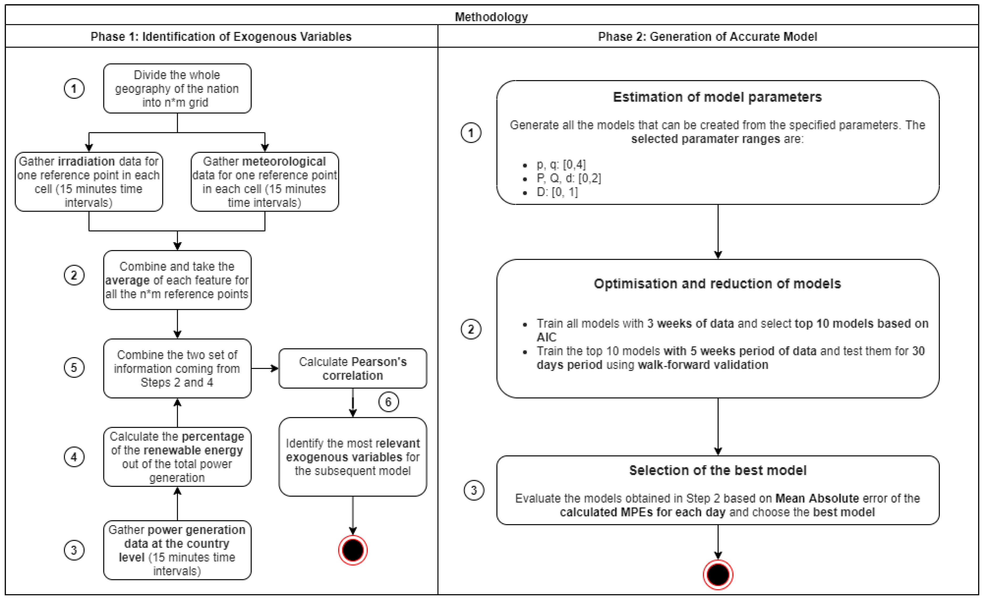
3. Proposed Methodology

In this section, the methodology used to generate prediction models for the percentage of renewables is described. As illustrated in Figure 1, the proposed methodology is based on two phases, where each such phase consists of several steps. These phases are organised in a sequential manner, such that each phase has a set of inputs and generates an output.

3.1. Phase 1: Identification of Exogenous Variables

As the first phase of the methodology, the choice of the exogenous variables has an important impact on the accuracy of the generated forecasting models. For this purpose, the main goal of this phase is to identify the set of exogenous variables relevant for the underlying model(s). Intuitively, a major aspect playing a role on the power generation of renewables is the information related to the meteorology and irradiation.

The generated forecast for the percentage of renewables needs to be realised at a macro-level (e.g., nation) instead of micro-level (e.g., region). This is because the percentage of renewables incorporates all the sources of green energy distributed among the borders of the largest administrative organisation, which is the country. Consequently, as the first step of this phase, the whole geography of the country is divided into a grid structure of n rows and m columns. Thus, this facilitates in specifying $n*m$ points such that each of those points can be used as a reference to collect meteorological as well as irradiation-related information. It is important to note that this information is re-sampled to 15-min resolution.

As a second step of this phase, this information (weather and irradiation) from the $n*m$ reference points is used to calculate their corresponding average values and standard deviations. The third step of this phase is to gather information related to the generated power with a resolution of 15 min. This information is used to calculate the percentage of renewables at the country level in the fourth step. Note that the percentage of RES is calculated as the ratio of power generated by RES to the total power produced by the different sources (with and without renewables). The two datasets derived in Steps 2 and 4 are then merged into a single one in the fifth step.

The final step (e.g., Step 6) of this phase consists of identifying the most relevant variables from irradiation and meteorological related information having influence on the generation of renewable energy sources. To achieve this, a Pearson’s correlation analysis (see Section 4) is carried out. Thus, the output of this phase is the set of exogenous variables extracted from irradiation and meteorological information that show linear correlation with respect to the percentage of renewable energy sources. This set of variables (see Section 4.3) will serve as an input to exogenous variables for the models based on SARIMAX and ARIMAX methods.

3.2. Phase 2: Generation of Accurate Model

The main objective of this phase is to generate the best accurate forecasting model for the method under study. For this purpose, as in the previous phase, this one is also composed of several sequential steps. The first step consists of estimating values of the model parameters corresponding to the method under study (e.g., SARIMAX, SARIMA, ARIMAX). Based on our literature review, the following range of values are defined:

• $p,q\in [0,4]$,
• $P,Q$ and $d\in [0,2]$,
• $D\in [0,1]$.

Note that the detailed explanation of the model parameters as well as the mathematical presentation of those methods can be found in Appendix A.2. While considering the different values within the above defined ranges, this leads to the generation of 1350 different models for SARIMA and SARIMAX and 75 different models for ARIMAX. Those ranges of values can generate models with the current hardware resources in a reasonable amount of time (see

Table 1. Execution times of the three time-series methods for Step 2 of Phase 2.

Method	Execution Time	Number of Models
SARIMAX	4 h and 30 min	1350
SARIMA	3 h	1350
ARIMAX	5 min	75

and

Table 2. Execution times of the three time-series methods for Step 3 of Phase 2.

Method	Execution Time	Number of Models
SARIMAX	3 h	10
SARIMA	1 h and 30 min	10
ARIMAX	1 h and 15 min	10

).

Thus, the second step of this phase is to perform optimisations and reduce the number of models generated in Step 1 for each method under study. To this end, first the different models obtained in Step 1 are trained with three weeks of data. AIC (Akaike’s Information Criterion) [33] is used in order to select the best 10 out of those different models (e.g., 1350 for SARIMA(X) and 75 for ARIMAX). To this end, AIC is an estimator that shows how good the model is trained, which is expressed as:

$$AIC=2k-2ln\left(\widehat{L}\right),$$

(1)

where k is the number of estimated parameters and $\widehat{L}$ is the maximum value of the likelihood function for the model. Then using the first 10 minimum AIC values from a set of candidate models, the 10 preferred ones are identified. After identifying the preferred 10 candidate models, Step 2 of this phase also consists of (1) training those models with a 5 week period of data and (2), testing them for a 30-days period using the walk-forward validation [25,32,34]. The reason for choosing a 30-day period is to generate forecasts for each month of the year.

In Step 3, the performance of the 10 models (coming out of Step 2) is compared using the mean absolute (MA) of the mean percentage error (MPE) obtained for each day (i.e., X in Equation (A13) is set to MPE). By the end of this phase, the most accurate model is obtained together with its optimal parameter sets (e.g., $p,q,P,Q,d$ and D) for the configured time-series method (e.g., SARIMAX, SARIMA, or ARIMAX) under study.

3.3. Comparison among Models

The above-mentioned methodology is used in order to carry out a comparison between the three methods of SARIMAX, SARIMA, and ARIMAX. Thus, the exogenous variables identified in Phase 1 of our methodology are used in SARIMAX and ARIMAX methods. Furthermore, Phase 2 is performed in three different iterations, such that each iteration implements one specific method of SARIMAX, SARIMA, and ARIMAX. The three best models each corresponding to the different methods of SARIMAX, SARIMA, and ARIMAX are then compared (see Section 5) to identify the best fitting one based on the considered assumptions and scenarios.

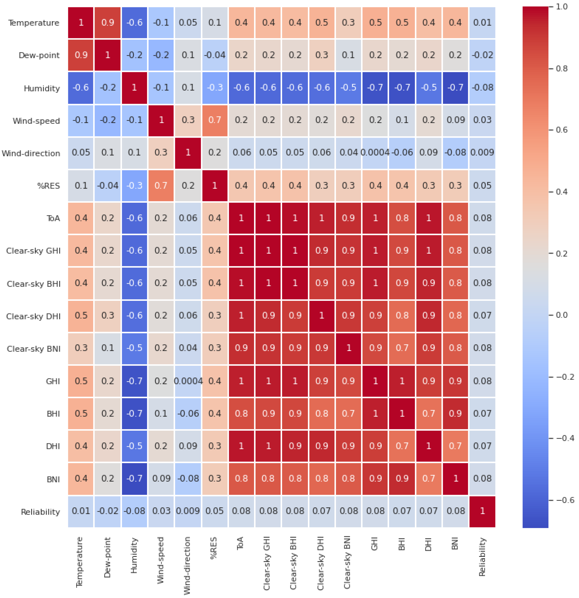
4. Correlation Analysis of the Features

In this section, first the mathematical definition of the Pearson’s correlation is given, then the used data is described, and the results of the carried-out analysis are presented. The obtained results give a clear indication of the exogenous variables—for the derived models using SARIMAX or ARIMAX methods—that can be used to predict the percentage of renewable energy sources.

4.1. Definition

Pearson’s correlation [35] is a measure of the linear correlation of two random variables, X and Y. It is calculated as the ratio of the covariance of those two variables to the product of their standard deviations:

$${\rho }_{X,Y}=\frac{cov(X,Y)}{{\sigma }_X{\sigma }_Y}$$

(2)

It ranges between −1, representing a total negative linear correlation, and 1, which is total positive linear correlation. A zero value indicates no correlation at all. Note that a linear correlation does neither indicate nor mean causality.

For this correlation analysis, the value of ${\rho }_{X,Y}$ needs to be found, such that X is the %RES (percentage of renewable energy sources), whereas Y can be any of the 15 variables from

Table 3. Variables and their explanations for irradiation related information.

Variable	Explanation and Unit
GHI	Global irradiation on a horizontal plane (Wh/m${}^2$)
BHI	Beam irradiation on a horizontal plane at ground level (Wh/m${}^2$)
DHI	Diffuse irradiation on a horizontal plane at ground level (Wh/m${}^2$)
BNI	Weather Beam irradiation on a mobile plane following the sun at normal incidence (Wh/m${}^2$)
ToA	Atmospheric radiation received by a horizontal surface outside the atmosphere (Wh/m${}^2$)
Reliability	Proportion of reliable data (0–1)
Clear-sky GHI	Clear-sky global irradiation on a horizontal plane at ground level (Wh/m${}^2$)
Clear-sky BHI	Clear-sky beam irradiation on horizontal plane at ground level (Wh/m${}^2$)
Clear-sky DHI	Clear-sky diffuse irradiation on horizontal plane at ground level (Wh/m${}^2$)
Clear-sky BNI	Clear-sky beam irradiation on a mobile plane following the sun at normal incidence (Wh/m${}^2$)

and

Table 4. Variables and their explanations for meteorology related information.

Variable	Explanation and Unit
Humidity	The ratio of partial to equilibrium pressure of water vapor at a given temperature (%)
Dew-point	Describes the amount of moisture in the air (mm${}^2$)
Temperature	Weather temperature (ºC)
Wind-speed	Wind flow speed (km/h)
Wind-direction	The direction from which the wind is coming from (degrees)

. Consequently, the input parameters for Equation (2) are X and Y, whereas the output is a value between −1 and 1 as explained above.

4.2. Data Sources

As mentioned above, the main objective of this analysis is to identify meteorology as well as irradiation-related variables that are positively correlated with the percentage of renewable energy sources that are distributed nation-wide. For this purpose, the geography of a nation is divided into n-by-m (e.g., Step 1 of Phase 1) grid. In our case, the percentage of renewables in Germany is considered. Thus, a 3-by-4 grid is specified and 12 representative cities (see red-colored regions in Figure 2) were selected, from which meteorological as well as irradiation related data were collected. It is important to mention that the selection of those representative cities is realised based on the following two constraints:

• The distance between any two points in the grid should not exceed 250 km. This is because, within a circular range of 250 km, the cities in this region have very similar weather conditions;
• Points as cities are chosen which have the least missing data from the collected sources, as well as preferably at the center of the circular region.

For the case of meteorology-related data, the Meteostat (https://dev.meteostat.net/api/ accessed on 5 November 2021) online service API was used to get historical data. For the irradiation, the open interface provided by SoDa-Pro (http://www.soda-pro.com/help/cams-services/cams-radiation-service/automatic-access accessed on 5 November 2021) was utilised together with the Copernicus Atmosphere Monitoring Service (CAMS) to fetch all data related to sky irradiation. Note that the observations of meteorology are in 1-h time intervals. However, due to the fact that the data related to renewable power generation are specified in 15-min time intervals, then the up-sampling technique [36] was used to increase the frequency of the weather data up to 15-min time intervals. Furthermore, the spline method [37] was utilised for the interpolation process. Regarding the percentage of renewables, the open API provided by European Network of Transmission System Operators for Electricity (ENTSOE) [38] was used. As mentioned above, this dataset is specified in the resolution of 15-minutes intervals. Finally, it is worthwhile to note that the collected data spanned from the period of 30 December 2017 until 10 July 2020. It consists of 88,702 data points and has a size of 10.3 MB (e.g., almost 2.5 years of information).

4.3. Correlated Variables

For the purpose of our modeling, two different features were considered to predict the percentage of renewable energy sources: irradiation and meteorology.

Regarding data related to irradiation, it contains 10 different variables, which are described in Table 3. Most of those variables are associated with the Horizontal Irradiation (HI), however, also taking into account different situations such as global, beam, diffuse, and their clear-sky counterparts. BNI and Clear-sky BNI denote respectively the beam irradiation at normal incidence and its clear-sky counterpart. ToA (Top of Atmosphere) denotes the atmospheric radiation received by a horizontal surface. All of those variables are expressed in terms of Wh/m${}^2$. Reliability variable is a factor between 0 and 1, which indicates the predictability that data exists (e.g., 1 showing 100% probability).

With respect to the data related to meteorology, it consists of five different variables, which are summarised in Table 4. Temperature describes the ambient temperature expressed in Celsius. The speed and direction of the wind are presented by the variables Wind-speed (in km/h) and Wind-direction (in degrees) respectively. The concentration of water vapor present in the air is given by the variable Humidity (in %). Dew-point describes the amount of moisture in the air (in mm${}^2$).

The percentage of the renewable energy sources is indicated by the variable %RES. To calculate its value, the following renewable sources are taken into account: biomass, hydro run-of-river and poundage, hydro water reservoir, geothermal, waste, other renewable sources, solar, hoffshore wind, and onshore wind. Consequently, the %RES is the ratio of the sum of generated power from those renewable sources to the total generation at the national level.

Figure 3 demonstrates the results of the Pearson’s correlation carried out on the variables of the two information of irradiation and meteorology given in Table 3 and Table 4 respectively, on the predictions of the renewable energy sources. Dark red color (between 0.7 and 1) shows a strong positive relationship, mild red color (between 0.3 and 0.7) presents a moderate positive relationship, and light red color (between 0 and 0.3) indicates a weak positive relationship. The dark, mild, and light blue colors are used to demonstrate the same behavior as the red ones, however for inverse correlation relationships. From the set of 15 observed variables, the carried out analysis indicates that this set of variables can be reduced to 2. More precisely, Wind-speed and %RES have a strong correlation of 0.7. On the other hand, among the irradiation related variables, apart from Reliability, all of them (9 variables from ToA till BNI) have a moderate positive correlation with %RES. Furthermore, GHI has a strong positive correlation with all other irradiation variables and also a weak positive correlation of 0.2 with Wind-speed. Hence, it could be argued that GHI is a suitable irradiation-related variable to predict %RES.

From the above given clarification on the carried-out Pearson’s correlation analysis, it can be concluded that both Wind-speed as well as GHI are identified as the two exogenous variables that can be served as input to the models (e.g., SARIMAX and ARIMAX) of Phase 2. As a side note, it is worthwhile to mention that during the performed analysis, it was observed that the amount of generated power from hydro water reservoir is low. However, the amount of generated power from hydro run-of-river and poundage is high. The wind speed indeed increases the water flow, which justifies our choice of Wind-speed for water-related renewable sources. Moreover, our analysis show that for the two identified exogenous variables of Wind-speed and GHI, there are always both historical (5 weeks back) as well as day-ahead forecasts.

5. Evaluation

In this section, the first details related to the considered hardware characteristics and the corresponding execution times for the different methods under study are given. Then, the obtained results of the carried-out experiments are presented by considering both intra- and inter-day scenarios.

5.1. Implementation

To generate the corresponding models, Phase 2 is executed on a machine with the following hardware characteristics:

• NVIDIA Tesla P100 GPU: base and maximum frequencies of 1190 MHz and 1330 MHz respectively;
• DRAM of 28 GB capacity: minimum and effective frequencies of 715 MHz and 1430 MHz respectively.

With the above-mentioned hardware characteristics, Table 1 and Table 2 summarise the execution times of the three time-series methods of SARIMAX, SARIMA, and ARIMAX for Steps 2 and 3 of Phase 2, respectively. It can be argued from those results that ARIMAX is the fastest because there is no seasonal parameter, whereas SARIMAX is the slowest one. Note that those execution times are needed only when a new model is generated. Once a suitable model is obtained, it takes around 2 min to generate day-ahead forecasts independent of the adopted method. To carry out statistical tests and perform statistical data exploration (e.g., calculation of AIC), we used Python’s statsmodel (https://www.statsmodels.org/stable/index.html accessed on 5 November 2021) library.

Furthermore, in this research, a Flask web service (Available at https://github.com/ren4kast/REN4KAST accessed on 5 November 2021) [39] was developed, which forecasts the percentage of renewable energy sources for the day ahead. The main service internally calls different services (the sources are mentioned above) to gather historical irradiance and meteorological data for the last 35 days starting from the previous day. Moreover, it collects real-time data for the current day as well as forecast data for the next day. It also gathers power generation data for the previous 35 days, and calculates the percentage of renewable energy sources. Sometimes, it happens that due to communication latency or error from sensors, some data points could be missing. To circumvent this problem, the developed service uses the last available data points. It is important to mention that this service is recommended to be used at the end of the current day as the most data points are available at this time of the day. Afterward, the best model for the current month (the best models for all months are given in

Table 5. Summary of the best ARIMA-based model for each month of the year. Table A1 reports the full results for different considered models.

Month	Model
January	SARIMA$(2,0,2)(2,1,1,4)$
February	ARIMAX$(2,0,4)$
March	ARIMAX$(4,0,3)$
April	SARIMAX$(4,1,3)(2,0,2,4)$
May	ARIMAX$(4,1,4)$
June	SARIMA$(4,1,3)(2,0,2,4)$
July	SARIMAX$(4,1,4)(1,0,1,4)$
August	SARIMA$(3,1,3)(2,0,2,4)$
September	SARIMAX$(3,1,1)(2,0,2,4)$
October	SARIMA$(4,1,3)(2,0,2,4)$
November	SARIMA$(3,1,3)(2,0,2,4)$
December	SARIMA$(3,1,4)(2,0,2,4)$

) is used to train it with the collected data, and forecast the percentage of renewable energy sources for the next day. This process can be executed very fast, and hence can generate results within minutes, as mentioned above.

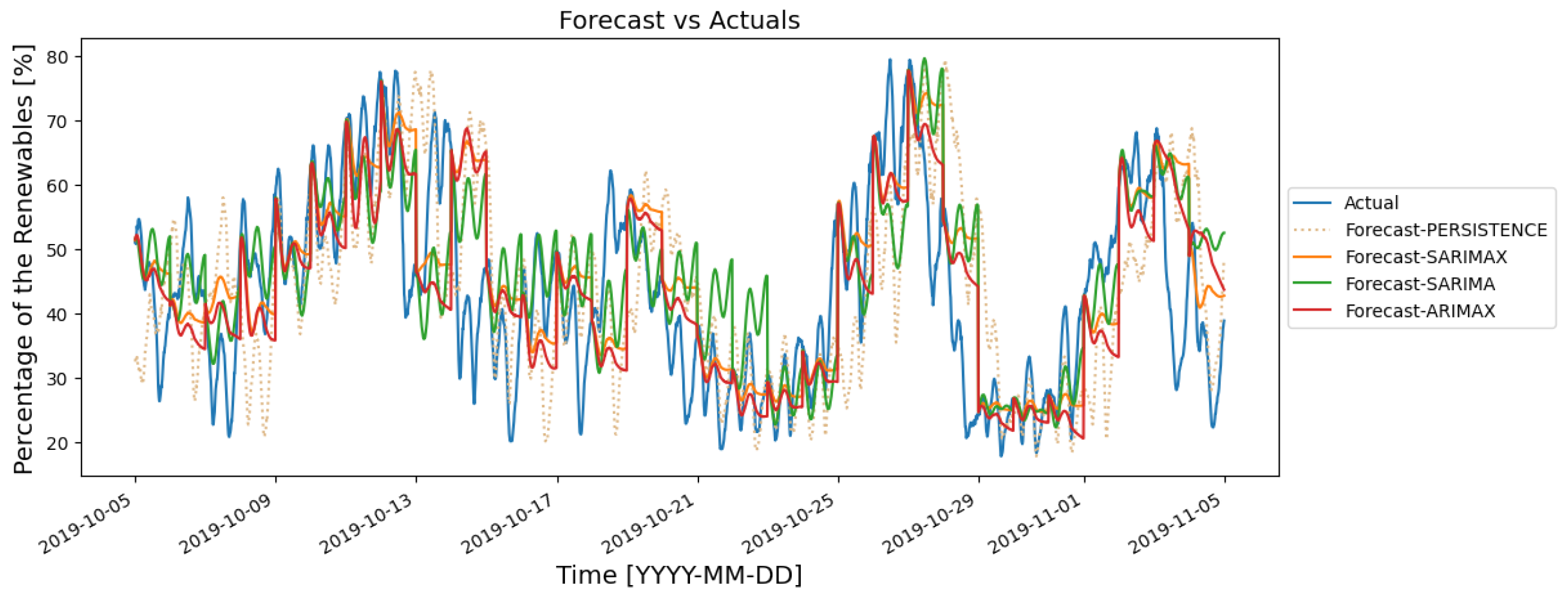
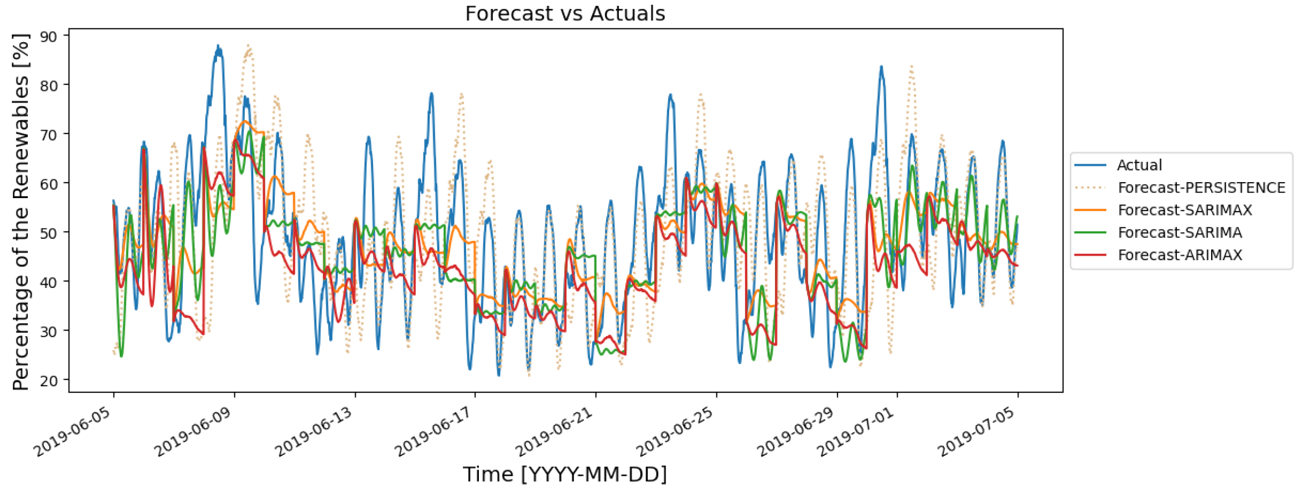
5.2. Obtained Results

In this section, the evaluation results of the methodology proposed in Section 3 are presented by considering a 30-day period in summer and autumn. This is because in summer there are longer sequential days with stable weather conditions, whereas in autumn more variations in meteorological data can be observed, which impact the power generation from renewables. Hence, both cases of varying and static weather conditions are studied. Readers interested in the whole months of the year can look at

Table A1. Comparison between ARIMA-based and persistence models for all months of the year. The results reported here are based on 4 different performance metrics.

Model—Month	Mean Absolute	Mean Absolute	Mean Absolute	Mean Absolute
	of the Errors [%]	of the MPEs [%]	of the RMSEs [%]	of the MAEs [%]
SARIMAX $(3,0,2)(2,1,2,4)$—January	7.69	28.09	10.06	8.70
SARIMA $(2,0,2)(2,1,1,4)$—January	7.64	26.30	10.03	8.62
ARIMAX $(3,0,4)$—January	8.33	23.07	10.60	9.19
Persistence—January	12.04	32.98	14.85	13.44
SARIMAX $(4,1,3)(1,0,0,4)$—February	6.18	18.20	9.15	7.66
SARIMA $(4,1,3)(1,0,0,4)$—February	5.92	17.52	9.23	7.63
ARIMAX $(2,0,4)$—February	6.03	14.78	9.01	7.39
Persistence—February	7.71	20.11	10.81	9.42
SARIMAX $(3,1,3)(2,0,2,4)$—March	7.43	14.94	10.41	8.43
SARIMA $(4,1,4)(2,0,2,4)$—March	7.26	14.68	10.64	8.57
ARIMAX $(4,0,3)$—March	6.88	13.53	10.35	8.10
Persistence—March	8.44	18.37	12.01	10.38
SARIMAX $(4,1,3)(2,0,2,4)$—April	4.60	9.73	8.40	6.76
SARIMA $(4,1,4)(2,0,2,4)$—April	6.35	12.22	9.27	7.53
ARIMAX $(4,1,4)$—April	4.47	10.03	8.80	7.11
Persistence—April	5.65	12.50	8.19	7.25
SARIMAX $(4,1,3)(2,0,2,4)$—May	7.89	15.88	11.77	9.69
SARIMA $(4,1,3)(2,0,2,4)$—May	9.85	19.09	13.24	11.08
ARIMAX $(4,1,4)$—May	7.09	14.79	11.53	9.35
Persistence—May	7.68	16.44	12.88	9.84
SARIMAX $(2,0,2)(2,1,2,4)$—June	6.54	15.76	12.46	10.15
SARIMA $(4,1,3)(2,0,2,4)$—June	6.32	13.25	11.32	9.40
ARIMAX $(2,1,3)$—June	8.59	17.32	14.26	11.57
Persistence—June	7.59	16.38	12.97	11.04
SARIMAX $(4,1,4)(1,0,1,4)$—July	5.03	12.96	10.66	8.68
SARIMA $(4,1,3)(2,0,2,4)$—July	4.99	11.50	11.01	8.88
ARIMAX $(3,1,3)$—July	5.64	12.06	10.97	8.74
Persistence—July	6.46	15.97	9.28	8.20
SARIMAX $(3,1,4)(2,0,2,4)$—August	5.56	11.88	12.19	9.57
SARIMA $(3,1,3)(2,0,2,4)$—August	4.87	12.75	10.17	8.14
ARIMAX $(4,1,3)$—August	6.16	13.11	12.63	9.91
Persistence—August	6.64	15.43	10.06	8.78
SARIMAX $(3,1,1)(2,0,2,4)$—September	6.38	15.12	10.16	8.21
SARIMA $(2,1,4)(2,0,2,4)$—September	6.41	14.79	10.02	8.22
ARIMAX $(3,1,2)$—September	6.57	15.96	11.22	8.95
Persistence—September	8.32	20.07	11.65	10.17
SARIMAX $(1,1,1)(2,0,2,4)$—October	6.80	18.54	9.23	7.80
SARIMA $(4,1,3)(2,0,2,4)$—October	6.54	18.46	8.95	7.48
ARIMAX $(3,1,4)$—October	7.20	19.88	10.34	8.58
Persistence—October	8.62	22.77	12.85	11.47
SARIMAX $(3,1,4)(2,0,2,4)$—November	8.81	29.61	11.13	9.42
SARIMA $(3,1,3)(2,0,2,4)$—November	8.34	28.58	10.69	9.03
ARIMAX $(3,1,4)$—November	8.51	28.63	10.93	9.22
Persistence—November	10.13	33.79	14.74	13.07
SARIMAX $(2,1,3)(0,0,2,4)$—December	10.48	26.01	13.20	11.29
SARIMA $(3,1,4)(2,0,2,4)$—December	10.03	24.71	12.75	10.91
ARIMAX $(4,1,3)$—December	10.45	25.83	13.20	11.32
Persistence—December	8.84	19.97	13.16	11.64

.

After selecting the top 10 candidates for each method, a set of 5-week periods of data was used to train the models and they were tested for the next 30 days (e.g., Step 2 of Phase 2). The walk-forward approach was used for testing: in each iteration, the model predicted the day ahead, and then this day was added to the training set to forecast the day after recursively.

For all the evaluation methods of the inter-day analysis, first the corresponding error metric (see Equations (A9)–(A12)) for each test day (intra-day) is calculated. Then, the mean absolute of the errors and MPE (which can be positive or negative) as well as the mean absolutes of RMSE and MAE (which are always positive numbers) for the 30 testing days (see Equation (A13)) are computed. Note that an MPE close to zero cannot be inferred as a very good model. Therefore, other evaluation metrics have been used to comprehensively evaluate and compare the models. On the other hand, intra-day analysis is performed by calculating the corresponding error metrics for one single day and considering 96 data points (e.g., 24 h and 15-min intervals). Finally, similar to [31], back-to-back similarity assumption (e.g., tomorrow’s forecast is the same as today) is considered as a baseline benchmark to provide a means of comparison with the derived three models of SARIMAX, SARIMA, and ARIMAX. Such a model is denoted as “persistence” and presented as dotted light orange line in the Figure 4, Figure 5, Figure 6 and Figure 7.

5.2.1. Inter-Day Analysis

Forecasting results for a period of one month in summer and autumn 2019 are depicted in Figure 4 and Figure 5, respectively. The first considerable difference is that in autumn, sharp changes could be observed by all models. However, all of these three models could not adapt themselves to the sharp changes happening during the day. This was detected when that day was added to the train data to predict the day after. In Figure 4, it could be observed that most of the time the SARIMAX forecast is between ARIMAX and SARIMA forecasts, which leads to a better mean absolute of MPEs (by considering the day and night changes).

It could be noted from

Table 6. Comparison between ARIMA-based and persistence models for the case of two different seasons of the year, and reporting the results of the inter-day scenario. The choice of the seasons is based on almost static (summer) vs. fluctuating (autumn) weather conditions.

Model	Mean Absolute	Mean Absolute	Mean Absolute	Mean Absolute
	of the Errors [%]	of the MPEs [%]	of the RMSEs [%]	of the MAEs [%]
SARIMAX$(2,1,2)(2,0,2,4)$ (summer)	4.76	9.97	10.51	8.30
SARIMA$(3,1,2)(2,0,2,4)$ (summer)	5.09	10.32	11.41	8.93
ARIMAX$(2,1,4)$ (summer)	4.78	10.25	10.54	8.31
Persistence (summer)	6.08	15.67	8.71	7.67
SARIMAX$(2,1,2)(0,0,2,4)$ (autumn)	7.07	19.46	10.35	8.58
SARIMA$(2,1,3)(2,0,2,4)$ (autumn)	7.23	19.56	9.57	8.15
ARIMAX$(3,1,4)$ (autumn)	7.36	20.14	10.48	8.74
Persistence (autumn)	9.35	23.92	12.88	11.63

that for both experiments in summer and autumn, SARIMAX performed better in terms of the mean absolute of the errors (i.e., X in Equation (A13) is set to $ME$). Furthermore, in summer and autumn on average every day, the predicted percentage of renewables could differ by 4.76% and 7.07% from the actual values, respectively. In general, the mean absolute of the errors in autumn is higher than in summer for all methods. This is due to detecting the sharp changes, however, with lags (as explained above). One interesting remark is that the means of the RMSEs and MAEs have slight differences between summer and autumn for all models (i.e., SARIMAX, SARIMA, and ARIMAX). However, those of MPE and ME have noticeably large differences. It implies that in summer, the intra-day errors (e.g., errors happening within one day) are distributed between positive and negative, so they cancel each other. However in autumn, since the model is lagged in detecting the changes (see Section 5.4.2 for reasons), the errors tend to be mostly in the same direction (positive or negative) so their effect is canceled less. The results for autumn show that SARIMAX is better than SARIMA in terms of the mean absolutes of the errors and MPEs (Columns 2 and 3 in Table 6). However, SARIMA is better in terms of the mean absolutes of the RMSEs and MAEs. This is because there are larger intra-day errors in SARIMAX forecasts that are canceling the effect of each other (for mean absolute of the errors and MPEs), whereas in SARIMA the errors are smaller.

5.2.2. Intra-Day Analysis

The best and the worst days of the testing period are depicted in

Table 7. A detailed analysis of the SARIMAX model for the best and worst days in summer. SARIMAX model is evaluated because it is shown in Table 6 that it has the best performance based on the Mean Absolute of the Errors (MAE) metric.

Model	Testing Date	Mean Error [%]	MPE [%]	RMSE [%]	MAE [%]
SARIMAX$(2,1,2)(2,0,2,4)$ (summer)	11 July2019	−0.40	−6.30	5.36	4.50
SARIMAX$(2,1,2)(2,0,2,4)$ (summer)	21 July 2019	8.39	2.57	19.47	16.82
SARIMAX$(2,1,2)(0,0,2,4)$ (autumn)	29 October 2019	−1.65	−8.41	3.25	2.44
SARIMAX$(2,1,2)(0,0,2,4)$ (autumn)	14 October 2019	−23.03	−63.23	25.05	23.03

for both summer and autumn based on MAE. The best MAE in autumn is 2.44%, which is better than the best MAE of 4.5% in summer. However, the worst MAE of summer is considerably better than the counterpart in autumn. On the worst day of autumn, a sharp change could be observed, and the model could not detect that. The SARIMAX model could not detect the changes during the day and is relatively predicting the average of the day. As a result, MAE is greater than the mean error, except for the worst day of the autumn experiment, where due to the sharp changes all the errors are in the same direction.

5.3. Sensitivity Analysis

The two methods of SARIMAX and ARIMAX require exogenous variables. It was shown in Section 4.3 that GHI and wind-speed can be used as the two exogenous variables for the two above-mentioned methods. To confirm the suitability of those variables as well as to evaluate the contribution of those exogenous variables to the methods, a sensitivity analysis is performed. The methodology in carrying out the corresponding analysis is to drop one of the two exogenous variables (e.g., GHI or wind-speed) and to generate the corresponding new model with one exogenous variable. After generating two different models, we compared the obtained forecasts using the performance metrics of the mean absolute of the errors, MPEs, RMSEs and MAEs, with the obtained models having both GHI and wind-speed as the two exogenous variables.

Table 8. Sensitivity Analysis of contribution of each variable. “Both” indicates GHI and wind-speed used together.

Model	Exogenous Variable(s)	Mean Error %	MPE	RMSE	MAE
January	Both	8.33	23.07	10.60	9.19
	GHI	8.36	21.73	10.80	9.25
	Wind-speed	8.27	22.78	10.57	9.15
February	Both	6.03	14.78	9.01	7.39
	GHI	6.51	18.00	9.27	7.84
	Wind-speed	6.11	15.45	9.26	7.52
March	Both	6.88	13.53	10.35	8.10
	GHI	xx	xx	xx	xx
	Wind-speed	6.87	13.59	10.70	8.37
April	Both	4.47	10.03	8.80	7.11
	GHI	4.55	10.09	8.85	7.14
	Wind-speed	4.79	10.36	9.61	7.63
May	Both	7.09	14.79	11.53	9.35
	GHI	7.23	15.11	11.69	9.49
	Wind-speed	7.45	14.84	12.59	10.19
June	Both	8.59	17.32	14.26	11.57
	GHI	8.70	17.45	14.36	11.65
	Wind-speed	9.03	17.43	15.05	12.17
July	Both	5.64	12.06	10.97	8.74
	GHI	5.73	12.20	11.08	8.84
	Wind-speed	6.19	12.18	12.23	9.73
August	Both	6.16	13.11	12.63	9.91
	GHI	6.79	14.31	13.16	10.44
	Wind-speed	5.26	12.63	13.01	10.57
September	Both	6.57	15.96	11.22	8.95
	GHI	6.60	15.98	11.32	9.04
	Wind-speed	5.26	12.63	13.01	10.57
October	Both	7.20	19.88	10.34	8.58
	GHI	7.08	19.66	10.35	8.58
	Wind-speed	7.59	19.76	12.09	9.68
November	Both	8.51	28.63	10.93	9.22
	GHI	8.56	28.77	10.96	9.26
	Wind-speed	8.30	28.12	10.76	9.04
December	Both	10.45	25.83	13.20	11.32
	GHI	10.43	25.76	13.14	11.28
	Wind-speed	10.06	25.01	12.83	10.92

illustrates the results of the carried-out sensitive analysis. The first column “Model” indicates the corresponding model for each month of the year. The second column “Exogenous Variable(s)” shows the used variables for the different models. “Both” indicate that the corresponding model takes into account both “GHI” and “wind-speed”, whereas “GHI” or “Wind-speed” denote that the model is generated using only one of them. It is worthwhile to note that the models are generated using the ARIMAX method and the data from the year 2019. Overall, looking at the results, it can be noticed that for most months of the year (except for November and December), models using both the GHI and wind-speed as exogenous variables have lower RMSE than when considering only one of them. Hence, the choice of both the GHI and wind-speed as exogenous variables for the two models of SARIMAX and ARIMAX can be justified.

5.4. Other Observations

In this section, building on the results demonstrated in Section 5.2, the results of another set of experiments are presented. Those observations were carried out in order to further state the theories derived previously.

5.4.1. Same Models for Different Years

The best model for each method (SARIMAX, ARIMAX, SARIMA) was chosen for a 30-day period between late spring and early summer 2019. Then, these models were used to predict the same period in 2020. The forecasts are depicted in Figure 6 and Figure 7, respectively. In addition, the evaluation results are shown in

Table 9. Comparison between ARIMA-based and persistence models for a 30-day period between late spring and early summer in 2019. The reported results for 2019 can be used to demonstrate the suitability of the same model to forecast the same period in 2020.

Model	Mean Absolute	Mean Absolute	Mean Absolute	Mean Absolute
	of the Errors [%]	of the MPEs [%]	of the RMSEs [%]	of the MAEs [%]
SARIMAX$(4,1,4)(2,0,0,4)$—(2019)	5.84	12.59	12.86	9.94
SARIMA$(3,1,4)(2,0,2,4)$—(2019)	6.52	13.99	12.32	10.08
ARIMAX$(4,0,3)$—(2019)	7.53	13.15	13.24	10.75
Persistence—(2019)	7.23	15.06	11.79	10.11
SARIMAX$(4,1,4)(2,0,0,4)$—(2020)	6.82	14.50	12.10	9.90
SARIMA$(3,1,4)(2,0,2,4)$—(2020)	7.95	15.05	12.98	12.54
ARIMAX$(4,0,3)$—(2020)	7.80	14.48	12.76	10.42
Persistence—(2020)	8.54	18.08	11.37	10.00

. It could be observed that SARIMAX outperformed ARIMAX and SARIMA in both 2019 and 2020. The mean absolute of the errors for SARIMAX is 5.84% in 2019 (where the best model was selected), and it increased to 6.82% in 2020. However, the mean of the MAEs remained almost the same. It means that in 2019, the errors were in different directions and canceled their effect. However in 2020, the errors were in the same direction, therefore the mean absolute of the errors is slightly higher. Hence, it can be conjectured that the proposed approach is appropriate to find the best model for each month. It can then be used to forecast the percentage of the renewables for the next years with an acceptable error rate.

5.4.2. Best Model of Each Month

Applying the methodology proposed in Section 3, the best model for each month of the year is identified, by considering the three methods of SARIMAX, SARIMA, and ARIMA. Table A1 shows the evaluation of the top models for each month, whereas Table 5 shows the derived (best) model for each month. In certain months, sharp changes have been observed (irregularities) for a few days, whereas the models could not detect them until the end of that day (as it was already discussed in Section 5.2.1 and Section 5.2.2). Most of those sharp changes are related to the changes in wind power generation. After careful analysis, the following fact can be identified: as a result of sharp changes in wind power generation, power system operators decided to increase/decrease the generation of fossil-based sources. This caused a sharper and sudden change in the percentage of renewable energy sources. For instance, on 19 November 2019 a sharp change can be observed. The reason is that on this day, fossil-based hard coal and gas generations increased from 4463 MW and 4481 MW to 12,054 MW and 8118 MW, respectively. In addition, the power generation from on- and off-shore wind sources decreased from 24,803 MW and 6076 MW to 1127 MW and 191 MW, respectively. It is worth mentioning that the mean values of the generation in 2019 from fossil-based hard coal and gas, as well as on- and off-shore wind sources are 6040.27 MW, 5684.41 MW, 11,397.19 MW, and 2606.76 MW, respectively.

In order to reduce the effect of the sudden change of generation from non-renewable sources, and also moderating those changes, the three worst months in terms of the mean absolute of the errors (from Table A1) were chosen and the methodology was followed to forecast the generation of renewables (instead of the percentage of the generation of renewables). In Section 5.4.3, more details will be given about the method and the results will be evaluated.

The selected models in Table 5 were used in the implemented service (https://github.com/ren4kast/REN4KAST accessed on 5 November 2021) to forecast the percentage of renewable energy sources for the day-ahead (see Section 5.1). The service is used to forecast the percentage of renewable energy sources from 24 November 2020 to 26 November 2020. The service was called every day at 11:50 p.m. to generate day-ahead forecasts. The results show that the mean of the MAEs, the mean of the RMSEs, and the mean absolute of the Errors for these three days were 5.10%, 5.73%, and 4.31% respectively, which are even better than their counterparts in 2019 (where the model was selected).

5.4.3. Forecasting Day-ahead Power Generation from Renewables

Table A1 demonstrates the different models based on the three time-series methods of SARIMAX, SARIMA, and ARIMAX for each month of the year. It can be noticed that the months of January, November, and December have the worst three prediction models. As mentioned above, it was found out that this is due to the fact that the operators increase/decrease the traditional fossil-based generation based on the contributions from renewable energy sources. To investigate more about this, instead of predicting the percentage of renewables (as is considered in Table A1), the power generation from renewables was predicted only for those three months (e.g., the three worst months). To do this, the same methodology provided in Section 3 was used, whereas the results are given in

Table 10. Evaluation of the best model candidates for forecasting the power generation of renewable energy sources.

Model	Mean Absolute	Mean Absolute	Mean Absolute	Mean Absolute
	of the Errors [MW]	of the MPEs [%]	of the RMSEs [MW]	of the MAEs [MW]
SARIMAX$(4,1,0)(0,1,1,4)$ (Jan.)	4280.23	16.23	5955.59	4885.47
SARIMA$(4,1,0)(2,0,2,4)$ (Jan.)	4308.06	16.36	6038.57	4927.70
ARIMAX$(3,1,1)$ (Jan.)	4285.68	16.15	5976.68	4905.17
SARIMAX$(3,2,1)(2,1,1,4)$ (Nov.)	7429.93	37.32	10,447.35	7905.16
SARIMA$(3,0,3)(2,0,1,4)$ (Nov.)	5502.95	26.49	7264.97	6045.49
ARIMAX$(3,2,2)$ (Nov.)	7042.42	35.12	9147.59	7401.43
SARIMAX$(3,1,4)(2,1,2,4)$ (Dec.)	5679.29	22.42	7172.82	6014.19
SARIMA$(3,1,1)(0,1,2,4)$ (Dec.)	5562.20	22.42	7172.64	6027.94
ARIMAX$(4,1,1)$ (Dec.)	5373.38	21.31	6970.78	5857.59

.

The results in Table 10 show that, the MPE is improved for all three months (in comparison with Table A1). More precisely, in January the MPE is improved by 10.07% (e.g., difference between 26.3% and 16.23%). However, in November and December improvements are less than in January, with 2.09% (e.g., difference between 28.58–26.49%) and 3.4% (e.g., between 24.71% and 21.31%).

To find out the reason for the 10.07% improvement in January, Pearson’s correlation between the variables was compared. In January, the generation of renewables was highly correlated to wind-speed, temperature, and dew-point with Pearson’s correlation of 0.9, 0.8, and 0.7, respectively. Additionally, temperature and dew-point were correlated to wind-speed with Pearson’s correlation of 0.7. Hence the wind-speed as an exogenous parameter perfectly covers renewables’ generation behavior. In November and December, power generation from renewables was highly correlated to wind-speed (0.9 and 0.8, respectively), but it was also correlated to other variables such as dew-point, temperature, and wind-direction (0.7, 0.8, and 0.5, respectively), as well as to humidity and temperature in December (−0.6 and 0.3, respectively). However, these variables are not correlated to wind-speed which is the model’s exogenous variable. Hence, the reason for drastic improvements in January can be justified.

6. Conclusions and Future Work

In this paper, the percentage of renewables at the national level is studied by considering different types of renewable energy sources. To achieve this, a two-phase methodology is proposed. Phase 1 deals with identifying the set of exogenous variables, and Phase 2 deals with the modelling of using them. It was showed that both GHI and wind-speed are consistently the two important exogenous variables that can be used to forecast the percentage of renewables from different types of sources. For modelling, the three different ARIMA (auto regressive integrated moving average) based methods were used and then optimised. Based on empirical results, it was shown that seasonal-based methods (e.g., SARIMA(X)) have the edge over non-seasonal method of ARIMAX for most of the months of the year. Further, it was conjectured that ARIMAX is better for the months where there are no sudden changes in the weather conditions. Finally, it was shown that our models have an accuracy between 6.76 and 11.57% for all months of the year. The best models were implemented in an open-source REN4KAST software platform.

Our developed method introduces promising preliminary results in the field of forecasting of renewables at a national level, and paves the way for future work, with real industrial impact such as within the context of electric mobility. Some of the limitations of our work are (1) the need to find statistical conditionals for each month and to choose exogenous variables, (2) lack of generalisable components as well as of parameter explicability, and (3) inconclusive hypothesis tests such as the p-test, leading to very large confidence intervals.

As for future work, it would be interesting to investigate the means of further improving the accuracy of those models and circumvent some of the above-mentioned limitations. To this end, it will be considered generating forecasts using AI-based methods such as LSTM (Long Short-Term Memory) and GRU (Gated Recurrent Units). Furthermore, our forecasting models will be incorporated within a real-life use case of electric-mobility, in order to demonstrate the added value as well as the need for our models with respect to planning and scheduling requirements.

References

1. Mehrasa, M.; Pouresmaeil, E.; Pournazarian, B.; Sepehr, A.; Marzband, M.; Catalão, J.P.S. Synchronous Resonant Control Technique to Address Power Grid Instability Problems Due to High Renewables Penetration. Energies 2018, 11, 2469. [Google Scholar] [CrossRef] [Green Version]
2. Basmadjian, R. Flexibility-Based Energy and Demand Management in Data Centers: A Case Study for Cloud Computing. Energies 2019, 12, 3301. [Google Scholar] [CrossRef] [Green Version]
3. Yukseltan, E.; Yucekaya, A.; Bilge, A.H. Hourly electricity demand forecasting using Fourier analysis with feedback. Energy Strategy Rev. 2020, 31, 100524. [Google Scholar] [CrossRef]
4. Ciechulski, T.; Osowski, S. High Precision LSTM Model for Short-Time Load Forecasting in Power Systems. Energies 2021, 14, 2983. [Google Scholar] [CrossRef]
5. Ciechulski, T.; Osowski, S. Deep Learning Approach to Power Demand Forecasting in Polish Power System. Energies 2020, 13, 6154. [Google Scholar] [CrossRef]
6. Zhang, D.; Tong, H.; Li, F.; Xiang, L.; Ding, X. An Ultra-Short-Term Electrical Load Forecasting Method Based on Temperature-Factor-Weight and LSTM Model. Energies 2020, 13, 4875. [Google Scholar] [CrossRef]
7. Li, R.; Chen, X.; Balezentis, T.; Streimikiene, D.; Niu, Z. Multi-step least squares support vector machine modeling approach for forecasting short-term electricity demand with application. Neural Comput. Appl. 2021, 33, 301–320. [Google Scholar] [CrossRef]
8. Jiang, P.; Li, R.; Lu, H.; Zhang, X. Modeling of electricity demand forecast for power system. Neural Comput. Appl. 2020, 32, 6857–6875. [Google Scholar] [CrossRef]
9. Basmadjian, R.; Kirpes, B.; Mrkos, J.; Cuchy, M. A Reference Architecture for Interoperable Reservation Systems in Electric Vehicle Charging. Smart Cities 2020, 3, 1405–1427. [Google Scholar] [CrossRef]
10. Eider, M.; Sellner, D.; Berl, A.; Basmadjian, R.; de Meer, H.; Klingert, S.; Schulze, T.; Kutzner, F.; Kacperski, C.; Stolba, M. Seamless Electromobility. In Proceedings of the Eighth International Conference on Future Energy Systems; ACM: New York, NY, USA, 2017; pp. 316–321. [Google Scholar]
11. Scheu, M.N.; Kolios, A.; Fischer, T.; Brennan, F. Influence of statistical uncertainty of component reliability estimations on offshore wind farm availability. Reliab. Eng. Syst. Saf. 2017, 168, 28–39. [Google Scholar] [CrossRef]
12. Neves, D.; Brito, M.C.; Silva, C.A. Impact of solar and wind forecast uncertainties on demand response of isolated microgrids. Renew. Energy 2016, 87, 1003–1015. [Google Scholar] [CrossRef]
13. González-Aparicio, I.; Zucker, A. Impact of wind power uncertainty forecasting on the market integration of wind energy in Spain. Appl. Energy 2015, 159, 334–349. [Google Scholar] [CrossRef]
14. Bauer, P.; Thorpe, A.; Brunet, G. The quiet revolution of numerical weather prediction. Nature 2015, 525, 47–55. [Google Scholar] [CrossRef] [PubMed]
15. Basmadjian, R.; de Meer, H. Evaluating and modeling power consumption of multi-core processors. In Proceedings of the 2012 Third International Conference on Future Systems: Where Energy, Computing and Communication Meet (e-Energy), Madrid, Spain, 9–11 May 2012; pp. 1–10. [Google Scholar] [CrossRef]
16. Basmadjian, R.; de Meer, H. Modelling and Analysing Conservative Governor of DVFS-Enabled Processors. In Proceedings of the Ninth International Conference on Future Energy Systems; Association for Computing Machinery: New York, NY, USA, 2018; pp. 519–525. [Google Scholar] [CrossRef]
17. Basmadjian, R.; Rainer, S.; Meer, H.D. A Generic Methodology to Derive Empirical Power Consumption Prediction Models for Multi-Core Processors. In Proceedings of the 2013 International Conference on Cloud and Green Computing, Karlsruhe, Germany, 30 September–2 October 2013; pp. 167–174. [Google Scholar] [CrossRef]
18. Lara-Benítez, P.; Carranza-García, M.; Luna-Romera, J.M.; Riquelme, J.C. Temporal Convolutional Networks Applied to Energy-Related Time Series Forecasting. Appl. Sci. 2020, 10, 2322. [Google Scholar] [CrossRef] [Green Version]
19. Ghofrani, M.; Suherli, A. Time series and renewable energy forecasting. Time Ser. Anal. Appl. 2017, 2017, 77–92. [Google Scholar]
20. Deb, C.; Zhang, F.; Yang, J.; Lee, S.E.; Shah, K.W. A review on time series forecasting techniques for building energy consumption. Renew. Sustain. Energy Rev. 2017, 74, 902–924. [Google Scholar] [CrossRef]
21. Hyndman, R.; Athanasopoulos, G. Forecasting: Principles and Practice, 2nd ed.; OTexts: Melbourne, Australia; Available online: OTexts.com/fpp2 (accessed on 5 November 2021).
22. Alsharif, M.H.; Younes, M.K.; Kim, J. Time series ARIMA model for prediction of daily and monthly average global solar radiation: The case study of Seoul, South Korea. Symmetry 2019, 11, 240. [Google Scholar] [CrossRef] [Green Version]
23. Atique, S.; Noureen, S.; Roy, V.; Subburaj, V.; Bayne, S.; Macfie, J. Forecasting of total daily solar energy generation using ARIMA: A case study. In Proceedings of the 2019 IEEE 9th annual computing and communication workshop and conference (CCWC), Las Vegas, NV, USA, 7–9 January 2019; pp. 0114–0119. [Google Scholar]
24. Vagropoulos, S.I.; Chouliaras, G.; Kardakos, E.G.; Simoglou, C.K.; Bakirtzis, A.G. Comparison of SARIMAX, SARIMA, modified SARIMA and ANN-based models for short-term PV generation forecasting. In Proceedings of the 2016 IEEE International Energy Conference (ENERGYCON), Leuven, Belgium, 4–8 April 2016; pp. 1–6. [Google Scholar]
25. Hodge, B.M.; Zeiler, A.; Brooks, D.; Blau, G.; Pekny, J.; Reklatis, G. Improved wind power forecasting with ARIMA models. In Computer Aided Chemical Engineering; Elsevier: Amsterdam, The Netherlands, 2011; Volume 29, pp. 1789–1793. [Google Scholar]
26. Basmadjian, R. Communication Vulnerabilities in Electric Mobility HCP Systems: A Semi-Quantitative Analysis. Smart Cities 2021, 4, 405–428. [Google Scholar] [CrossRef]
27. Kirpes, B.; Danner, P.; Basmadjian, R.; de Meer, H.; Becker, C. E-Mobility Systems Architecture: A Framework for Managing Complexity and Interoperability. Energy Inform. 2019, 2, 15. [Google Scholar] [CrossRef]
28. Hassan, M.Z.; Ali, M.E.K.; Ali, A.S.; Kumar, J. Forecasting day-ahead solar radiation using machine learning approach. In Proceedings of the 2017 4th Asia-Pacific World Congress on Computer Science and Engineering (APWC on CSE), Mana Island, Fiji, 11–13 December 2017; pp. 252–258. [Google Scholar]
29. Singh, V.P.; Vijay, V.; Bhatt, M.S.; Chaturvedi, D. Generalized neural network methodology for short term solar power forecasting. In Proceedings of the 2013 13th International Conference on Environment and Electrical Engineering (EEEIC), Wroclaw, Poland, 1–3 November 2013; pp. 58–62. [Google Scholar]
30. Basmadjian, R.; De Meer, H. A Heuristics-Based Policy to Reduce the Curtailment of Solar-Power Generation Empowered by Energy-Storage Systems. Electronics 2018, 7, 349. [Google Scholar] [CrossRef] [Green Version]
31. Basmadjian, R. Optimized Charging of PV-Batteries for Households Using Real-Time Pricing Scheme: A Model and Heuristics-Based Implementation. Electronics 2020, 9, 113. [Google Scholar] [CrossRef] [Green Version]
32. Eldali, F.A.; Hansen, T.M.; Suryanarayanan, S.; Chong, E.K. Employing ARIMA models to improve wind power forecasts: A case study in ERCOT. In Proceedings of the 2016 North American Power Symposium (NAPS), Denver, CO, USA, 18–20 September 2016; pp. 1–6. [Google Scholar]
33. Akaike, H. A new look at the statistical model identification. IEEE Trans. Autom. Control 1974, 19, 716–723. [Google Scholar] [CrossRef]
34. Mishra, A.; Desai, V. Drought forecasting using stochastic models. Stoch. Environ. Res. Risk Assess. 2005, 19, 326–339. [Google Scholar] [CrossRef]
35. Pearson, K. Notes on the History of Correlation. Biometrika 1920, 13, 25–45. [Google Scholar] [CrossRef]
36. Brownlee, J. Introduction to Time Series Forecasting with Python: How to Prepare Data and Develop Models to Predict the Future; Machine Learning Mastery, 2017; Available online: https://books.google.de/books?id=bA5ItAEACAAJ (accessed on 5 November 2021).
37. Demirhan, H.; Renwick, Z. Missing value imputation for short to mid-term horizontal solar irradiance data. Appl. Energy 2018, 225, 998–1012. [Google Scholar] [CrossRef]
38. European Network of Transmission System Operators for Electricity (Enstoe). Available online: https://transparency.entsoe.eu/ (accessed on 5 November 2021).
39. Grinberg, M. Flask Web Development: Developing Web Applications with Python; O’Reilly Media, Inc.: Sebastopol, CA, USA, 2018. [Google Scholar]
40. Kattan, A.; Fatima, S.; Arif, M. Time-series event-based prediction: An unsupervised learning framework based on genetic programming. Inf. Sci. 2015, 301, 99–123. [Google Scholar] [CrossRef]
Figure 1. The two phases of the proposed methodology with their corresponding steps.
Energies 14 07443 g001
Figure 2. The distribution of the reference points (cities) used to gather meteorological and irradiation related data.
Energies 14 07443 g002
Figure 3. Results of the Pearson’s correlation analysis regarding the exogenous variables of irradiation and meteorology on the percentage of renewable energy sources.
Energies 14 07443 g003
Figure 4. Forecasts for a one month period in summer 2019.
Energies 14 07443 g004
Figure 5. Forecasts for a one month period in autumn 2019.
Energies 14 07443 g005
Figure 6. Forecasts for a one month period between late spring and early summer 2019.
Energies 14 07443 g006
Figure 7. Forecasts for a one month period between late spring and early summer 2020.
Energies 14 07443 g007