Article

3DHIP-Calculator—A New Tool to Stochastically Assess Deep Geothermal Potential Using the Heat-In-Place Method from Voxel-Based 3D Geological Models

1
Departament de Geologia, Universitat Autònoma de Barcelona (UAB), 08193 Barcelona, Spain
2
Àrea de Recursos Geològics, Institut Cartogràfic i Geològic de Catalunya (ICGC), 08038 Barcelona, Spain
3
Departament de Mineralogia, Petrologia i Geologia Aplicada, Facultat de Ciències de la Terra, Universitat de Barcelona (UB), 08028 Barcelona, Spain
*
Author to whom correspondence should be addressed.
Energies 2021, 14(21), 7338; https://doi.org/10.3390/en14217338
Submission received: 11 September 2021 / Revised: 25 October 2021 / Accepted: 2 November 2021 / Published: 4 November 2021

Abstract

:
The assessment of the deep geothermal potential is an essential task during the early phases of any geothermal project. The well-known “Heat-In-Place” volumetric method is the most widely used technique to estimate the available stored heat and the recoverable heat fraction of deep geothermal reservoirs at the regional scale. Different commercial and open-source software packages have been used to date to estimate these parameters. However, these tools are either not freely available, can only consider the entire reservoir volume or a specific part as a single-voxel model, or are restricted to certain geographical areas. The 3DHIP-Calculator tool presented in this contribution is an open-source software designed for the assessment of the deep geothermal potential at the regional scale using the volumetric method based on a stochastic approach. The tool estimates the Heat-In-Place and recoverable thermal energy using 3D geological and 3D thermal voxel models as input data. The 3DHIP-Calculator includes an easy-to-use graphical user interface (GUI) for visualizing and exporting the results to files for further postprocessing, including GIS-based map generation. The use and functionalities of the 3DHIP-Calculator are demonstrated through a case study of the Reus-Valls sedimentary basin (NE, Spain).

1. Introduction

Deep geothermal energy exploration and exploitation activities have vigorously grown during the last decade worldwide [1,2,3]. One of the key tasks during the early evaluation stages of deep geothermal plays is the assessment of the base resource in terms of the energy stored in the reservoir [4]. This quantification is an essential step to estimate the energy that can be produced from the geothermal reservoir for power generation or direct uses (district heating, greenhouses, etc.), and is key for carrying out preliminary evaluations of the project feasibility based on the required investment and the exploitation cost of the geothermal resource. However, there are uncertainties in the geological knowledge that must be considered when carrying out these preliminary assessments during the early stages of exploration of the geothermal resource. These uncertainties are mainly related to the prediction of the reservoir geometry, petrophysical properties, and temperature distribution.
The volumetric “Heat-In-Place” (HIP) method, implemented by the United States Geological Survey (USGS) [5], together with its subsequent revisions [6,7,8,9,10], is still the most widely used evaluation technique for the estimation of the available stored heat and the recoverable heat fraction (Hrec) of deep geothermal reservoirs [11,12,13,14,15,16]. This method considers the volume of the reservoir (surface and thickness), the petrophysical properties (e.g., rock type, porosity, specific heat capacity, etc.), fluid properties (e.g., fluid density, etc.), as well as the reservoir and reinjection (or reference) temperatures. Due to the potential influence of these parameters and their uncertainty, Nathenson [17] considered the need to follow a stochastic approach through Monte Carlo simulations [18]. This approach systematically varies the parameters considered over a defined range of values by using probability distribution functions (PDF) (e.g., triangular, normal, lognormal, etc.) [8,19,20].
Traditionally, common commercial software designed for risk and decision analysis purposes, such as @Risk [21] and Crystal Ball [22], have been used for geothermal resource assessment. They apply the volumetric method using Monte Carlo simulations (i.e., stochastic calculations implementing PDFs for the variables). Both tools run as Microsoft Excel add-ins, and calculations are normally applied at the scale of the entire reservoir or to a specific part of it, where the selected volume is conceptually treated as a single voxel [23,24,25,26]. In terms of open-source software, Pocasangre et al. [27] have more recently developed the ‘GPPeval’ application (Geothermal Power Potential assessment), a Python-based stochastic library for the assessment of the geothermal power potential using the volumetric method in a liquid-dominated reservoir. A handicap of these applications is that the analyzed domain must be treated as a lumped parameter model, i.e., with a homogeneous distribution of parameters in the whole volume considered. However, local variabilities are expected in reservoirs, mainly due to the variation of the petrophysical properties, temperature distribution, and reservoir geometry (thickness, depth, etc.). For this reason, approaches based on GIS (Geographic Information System) coupled with 3D subsurface models are promising, because they explicitly allow the application of the volumetric method using 3D voxel models as inputs. Several authors have used 3D geological models to calculate the volume of a reservoir to subsequently apply the HIP volumetric method in a deterministic way by assigning values to parameters of each unit to estimate, quantify, and map a first estimation of the geothermal reserve [28,29].
A more sophisticated approach is that applied by the VIGORThermoGIS code [12], an implementation of the ThermoGIS TNO code [30,31,32]. This tool was implemented specifically to assess prospective areas for geothermal development in the Netherlands and in southern Italy during the VIGOR Project [12]. The codes and the methodology implemented in these two tools can be considered nowadays as a reference for the scientific community working on the evaluation of resources at the regional scale. These tools demonstrated the use of methods that couple 3D subsurface data with GIS tools to stochastically assess the deep geothermal potential. Nevertheless, their implementation was limited to their case study areas and specific datasets. Therefore, there is still a need for a standard and freely available tool for the whole geothermal community in order to be able to estimate the HIP using Monte Carlo simulations, and in which any 3D geological and 3D thermal models can be utilized to assess case studies.
A gap is identified between what the geoscience community working in geothermal energy would need (including geological surveys, universities, research institutes, or consulting companies) and what is currently offered by free commercial or open-source software packages to assess deep geothermal potential at the regional scale in three-dimensions and by stochastically using the volumetric method. To close this gap, a novel and free software called the ‘3DHIP-Calculator’ is presented here. This tool allows for estimating the geothermal potential of a reservoir using the volumetric Heat-In-Place (HIP) method, originally implemented by the United States Geological Survey (USGS) [5], combined with a Monte Carlo simulation approach [17] and using 3D geological and 3D thermal models based on a voxel format as inputs.
The 3DHIP-Calculator application has many competitive advantages. Firstly, the source code and the installation files are accessible for all users and developers from open-source repositories such as GitHub. Secondly, as the tool allows importing 3D models that integrate previously generated geological, petrophysical, and thermal data, it considers the whole geological heterogeneity of the reservoir to estimate the geothermal potential using the HIP method. Finally, the results can be exported in ASCII format for their subsequent post-processing in other environments, such as GIS software packages. This allows generating maps of the assessed deep geothermal potential at the regional scale, and to use 3D visualization tools and statistical packages, such as R [33], for further evaluations. All these advantages open a wide range of possibilities, including the construction of GIS-based maps or to conduct feasibility studies of the deep geothermal potential through risk analysis approaches.
This contribution presents the structure, capabilities, and use of the 3DHIP-Calculator and its graphical user interface (GUI). Moreover, the method is demonstrated through a case study of the Reus-Valls Basin (RVB) [34]. The RVB is part of the Neogene extensional basins of the Catalan Coastal Ranges (NE of the Iberian Peninsula, Spain), which, according to previous studies [35,36,37], has a high potential for the development of deep geothermal energy for direct heat or power generation. However, the lack of enough subsurface information (from deep appraisal wells) results in a relatively large uncertainty for the assessment of its geothermal potential. The RVB case is a useful example of deep geothermal potential assessment at the regional scale, where the 3DHIP-Calculator can offer a first estimate of the spatial distribution of the deep geothermal resource based on the existing geological knowledge and its associated uncertainty.

2. Materials and Methods

2.1. Mathematical Background of the HIP Method

The 3DHIP-Calculator is based on the HIP approach, which allows estimating the geothermal resource and the recoverable fraction of a subsurface reservoir [5,10,11,12]. The HIP (kJ) is calculated according to Equation (1):
HIP = V · · ρ F · C F + 1 · ρ R · C R · T r T i
where V is the voxel volume (m3), is the rock porosity (parts per unit), ρ is the rock density (kg/m3), C is the specific heat capacity (kJ/kg·°C), and the F and R sub-indexes account for the fluid and host rock, respectively. Tr is the reservoir temperature (°C) and Ti refers to either the re-injection, reference, or abandonment temperature (°C). Therefore, Ti can refer to the threshold of economic or technological viable temperature, the ambient temperature (i.e., the annual mean surface temperature value), or a temperature value defined according to other criteria [11]. Equation (1) is solved within the 3DHIP-Calculator for each voxel in the model that satisfies the condition that T r T i 5   ° C . Otherwise, the HIP for that voxel is not evaluated and is set to zero. The HIP is expressed in kJ.
Then, the obtained HIP value is used to calculate the recoverable heat (Hrec) following Equation (2), which accounts for the producible thermal power during a given plant or project lifetime (Tlive):
Hrec = HIP · C e · R T l i v e · P f
where the HIP resulting from Equation (1) is scaled by a recovery factor (R, in parts per unit) to represent the part of the heat that can be extracted. This first estimation of the recovery factor (R) requires special attention because it depends on many factors, including the hydrogeological characteristics of the reservoir and the current drilling technology. Some authors suggest using R values between 0.02 and 0.2 [38] or close to 0.01 [12] for studies where there is no previous information. A recovery factor for a geothermal doublet (with a production borehole and an injection borehole) was defined at 0.33 according to the Atlas of Geothermal Resources in Europe [16,39], based on Muffler and Cataldi [5] and Lavigne [40]. Williams et al. [6,7,41] proposed a range of R values according to the geothermal reservoir type: a range from 0.08 to 0.2 for fracture-dominated reservoirs, 0.01 for Enhanced Geothermal Systems [42], and from 0.1 to 0.25 for sediment-hosted reservoirs with a maximum value of 0.5 [3]. Additionally, a conversion efficiency factor (Ce, in parts per unit) is used to incorporate the effect of the efficiency of the heat exchange from the geothermal fluid to a secondary fluid in a thermal plant. Ce can vary as a function of geothermal exploitation (e.g., heat or electricity production). Finally, since most of the direct heat applications of geothermal energy (such as district heating, greenhouse heating, etc.) do not operate continuously throughout the year, a plant factor (Pf, in parts per unit) is included. This factor considers the fraction of the total time in which the geothermal plant is in operation. Thus, Hrec is expressed in kW.

2.2. Mathematical Background of the Monte Carlo Method

The Monte Carlo method, i.e., a multiple probability simulation, is a mathematical solution widely used to estimate the possible outcomes of an uncertain event. Unlike a normal forecasting model, Monte Carlo simulations predict a set of outcomes based on an estimated range of values versus a deterministic or fixed input value. This method is used in the 3DHIP-Calculator to probabilistically evaluate the uncertainty associated with the input parameters and the corresponding geothermal potential results [18]. The first step is to link a probability distribution function (PDF) to each parameter, to infer the unknown quantities of the samples, and to take into account the range and pattern of variation of the different parameters [43]. Thus, Equations (1) and (2) are applied using a stochastic approach, instead of a deterministic one, so that their input values are not fixed parameters yielding a unique result. The calculations based on these two equations are repeated as many times as desired (N, number of simulations), producing a large number of likely outcomes, using random values extracted from probability distribution functions assigned to the parameters and predefined depending on the pattern variation. The application allows selecting normal or triangular PDFs for the input parameters of Equations (1) and (2). The mean and standard deviation are used to define normal distributions, while the lower, most probable, and upper values are for triangular distributions. The required input data for the calculations are 3D geological models (3DGM), 3D thermal models (3DTM), and random values within the selected PDF for each parameter. The values of the variables defined in a deterministic way (i.e., without assigning PDFs) are considered as fixed. Accordingly, the application calculates as many different HIP and Hrec values as the number of simulations defined by the user for each voxel of the model. The results of the calculations are also expressed as PDFs.

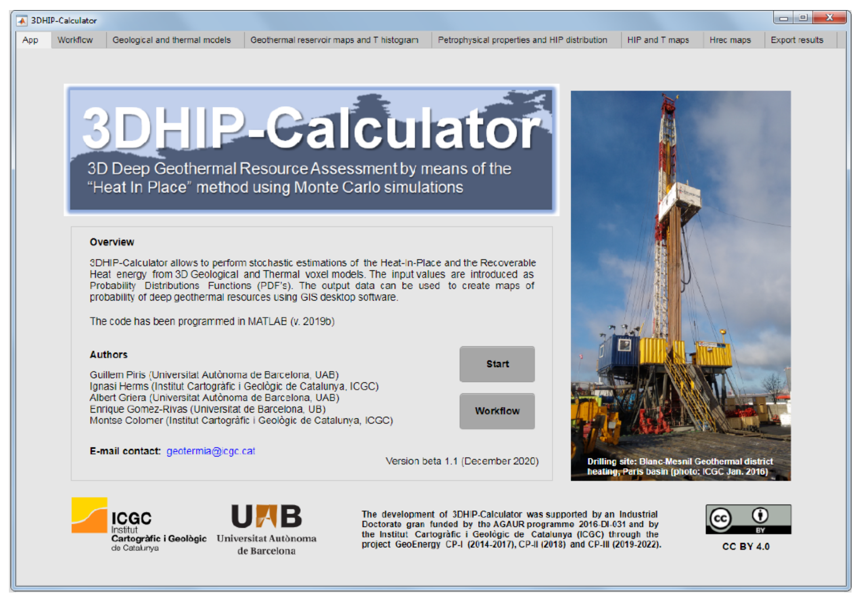
2.3. Program Description

The 3DHIP-Calculator (Figure 1) was developed using MATLAB ® (v. R2019b) [44] based on the MATLAB App Designer, and then compiled for Windows as a standalone application. The installation files, as well as the user manual and examples, can be freely downloaded from the “Deep geothermal energy” web page of the Institut Cartogràfic i Geològic de Catalunya (ICGC) (under the Creative Commons license Attribution 4.0 International, CC BY 4.0). The source code can also be downloaded from https://github.com/OpenICGC/3DHIP-Calculator (accessed on 15 October 2021).
An easy-to-use graphical user interface (GUI) was implemented and organized in six main steps, as shown in the workflow of Figure 2. The first part comprises the pre-processing step, that includes the selection of input parameters (step 1 in Figure 2). In this step, the input 3D geological and 3D thermal models (referred to as 3DGM and 3DTM, respectively) are converted to a matrix, where each row corresponds to one voxel in the 3D model and the columns are the petrophysical/reservoir parameters. Using depth ranges and geological units, the target volume of the whole model is defined. The parameters that are not included as initial data in the 3D models are defined using PDFs (2, Figure 2).
During the processing step, the HIP and Hrec calculations are carried out using Equations (1) and (2), and performed as many times (N) as desired (3, Figure 2). The full results from the N simulations are stored for each voxel of the model and include the entire uncertainty obtained from the Monte Carlo method. Then, the results are statistically compiled to obtain a cumulative probability distribution (CDF) for each voxel, from which the representative probability values are extracted. The voxels corresponding to the target volume are also summed and compiled statistically to obtain the probability results for the entire target reservoir (4, Figure 2). Finally, the post-processing allows visualizing the probability results (4 and 5, Figure 2) and exporting the original data and the stochastic results to ASCII files (6, Figure 2).

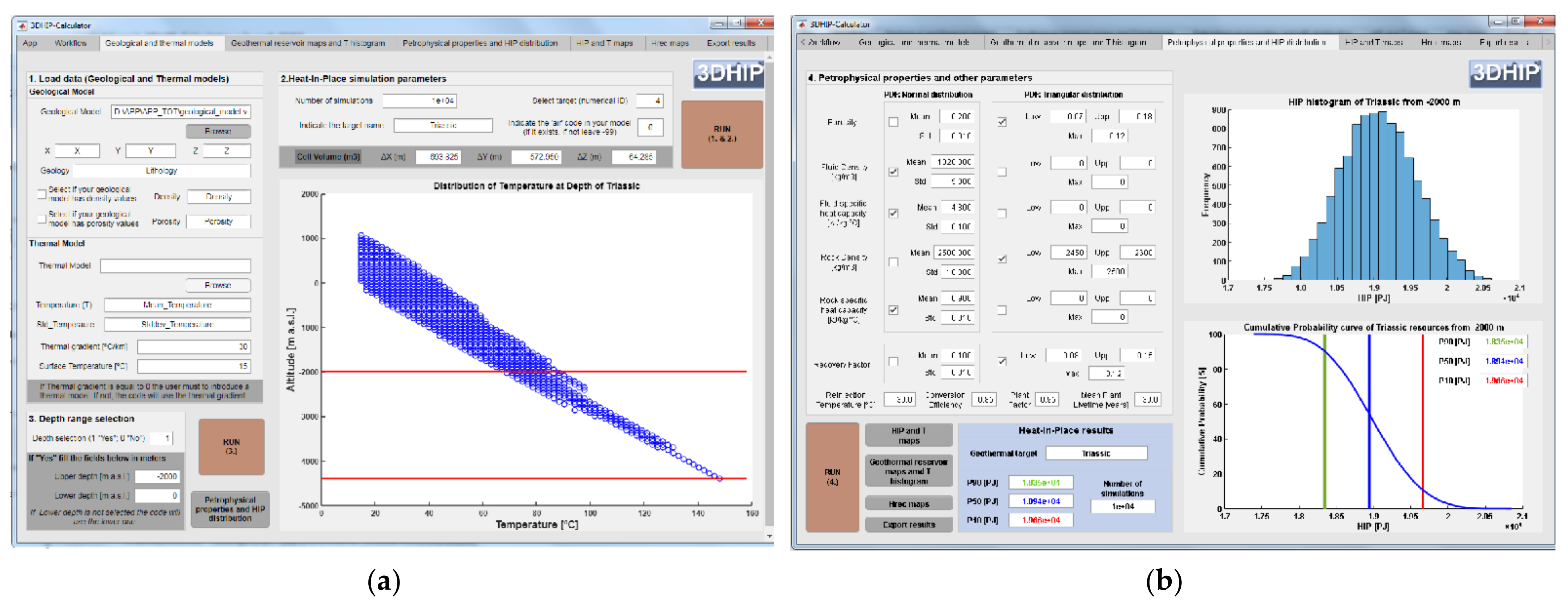
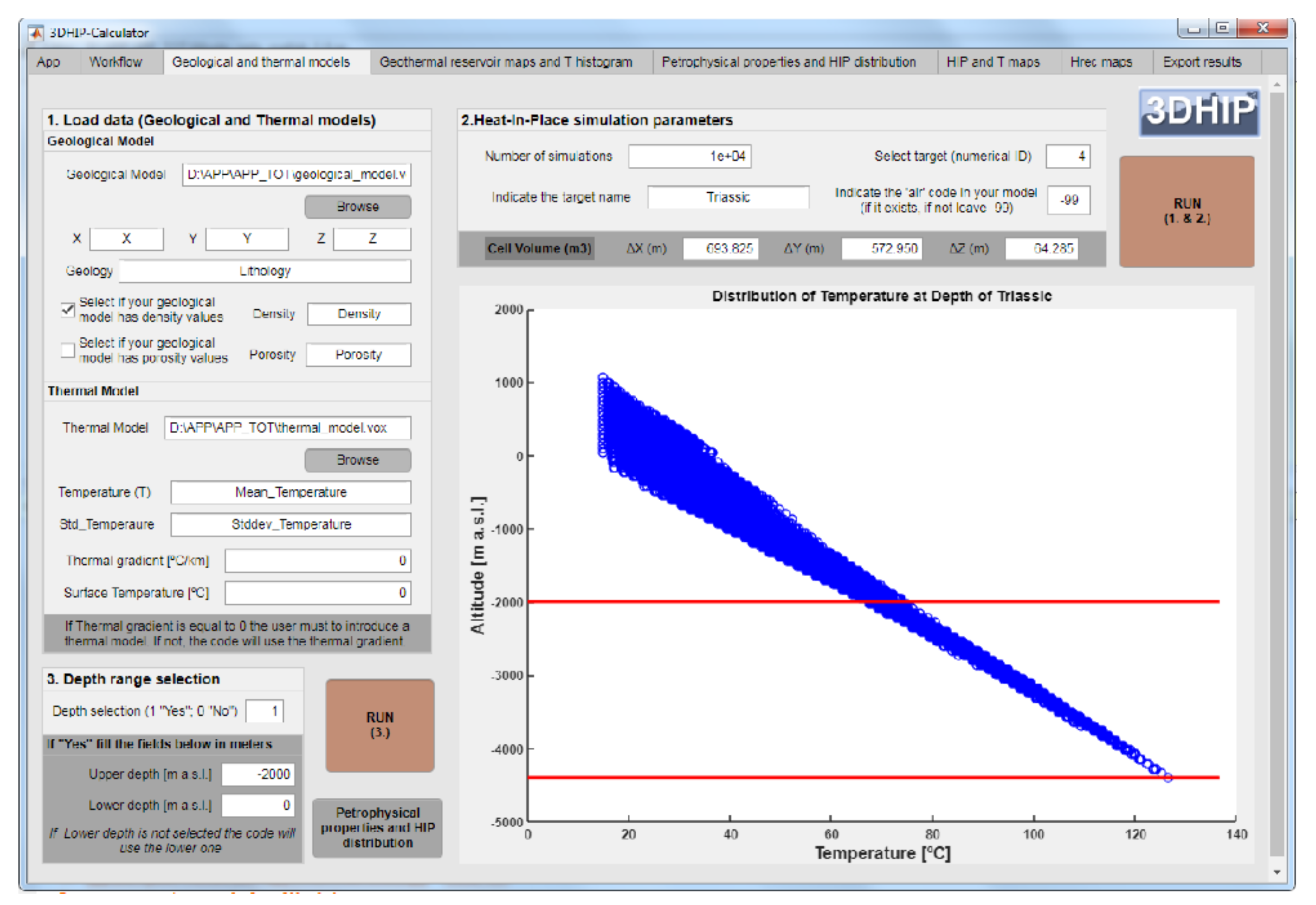
2.3.1. Pre-Processing: Input Data

An essential step to run the application is to choose and upload the imported 3DGM and 3DTM. The application allows for loading data using ASCII text files, delimited by tabulators, spaces, or commas. A 3DTM is not always required, and alternatively, an approach based on a linear geothermal gradient according to depth can be used, if a 3DTM is not available. When this option is chosen, the temperature of each voxel is calculated according to Equation (3):
Tz = T0 + ΔT × Dz
where Tz is the estimated temperature at depth z, T0 is the mean annual surface temperature, ΔT is the measured thermal regional gradient in C/km, and Dz is the depth z of the target according to the preliminary 3D model. This approach assumes a conductive steady-state regime and is indicated for geothermal plays in passive tectonic settings where no asthenospheric anomalies occur [45].
The 3DGM and 3DTM files should follow certain rules in terms of data organization (e.g., Figure 3). Particularly, they need to include at least one line of column headers before listing the data. The file is organized in a way that each column contains a variable, and each line corresponds to a voxel. The columns normally correspond to (in this order): voxel coordinates (X, Y, and Z, usually corresponding to its centroid) in UTM or geographic coordinates in decimal degrees, and a numerical identifier to differentiate the geological units (e.g., lithology, formation, reservoir, target, etc.). Additionally, the 3DGM can contain petrophysical parameters such as density (in g/cm3) and porosity (parts per unit) that can vary for each voxel. The 3DTM should include the voxel coordinates (X, Y, and Z), the temperature (in °C), and the temperature standard deviation (in °C) for each voxel. The temperature standard deviation is an optional parameter that can be set to zero if it is unknown. Furthermore, the voxel position and resolution (in X, Y, and Z) of the geological and thermal models must be identical and match each other.
These input files for the voxel-based 3DGM and 3DTM can be generated using common commercial geological modeling software, such as GeoModeller3D (©BRGM, Intrepid-Geophysics) or SKUA-GOCAD® (Paradigm), or GemPy, an open-source 3D geological model based on Python [46], among many other packages able to export 3D models in this format. The files for the testing case presented in this paper were generated using GeoModeller3D (v4.0.8).

2.3.2. Post-Processing: Output Data

The outputs from the stochastic simulations are utilized to:
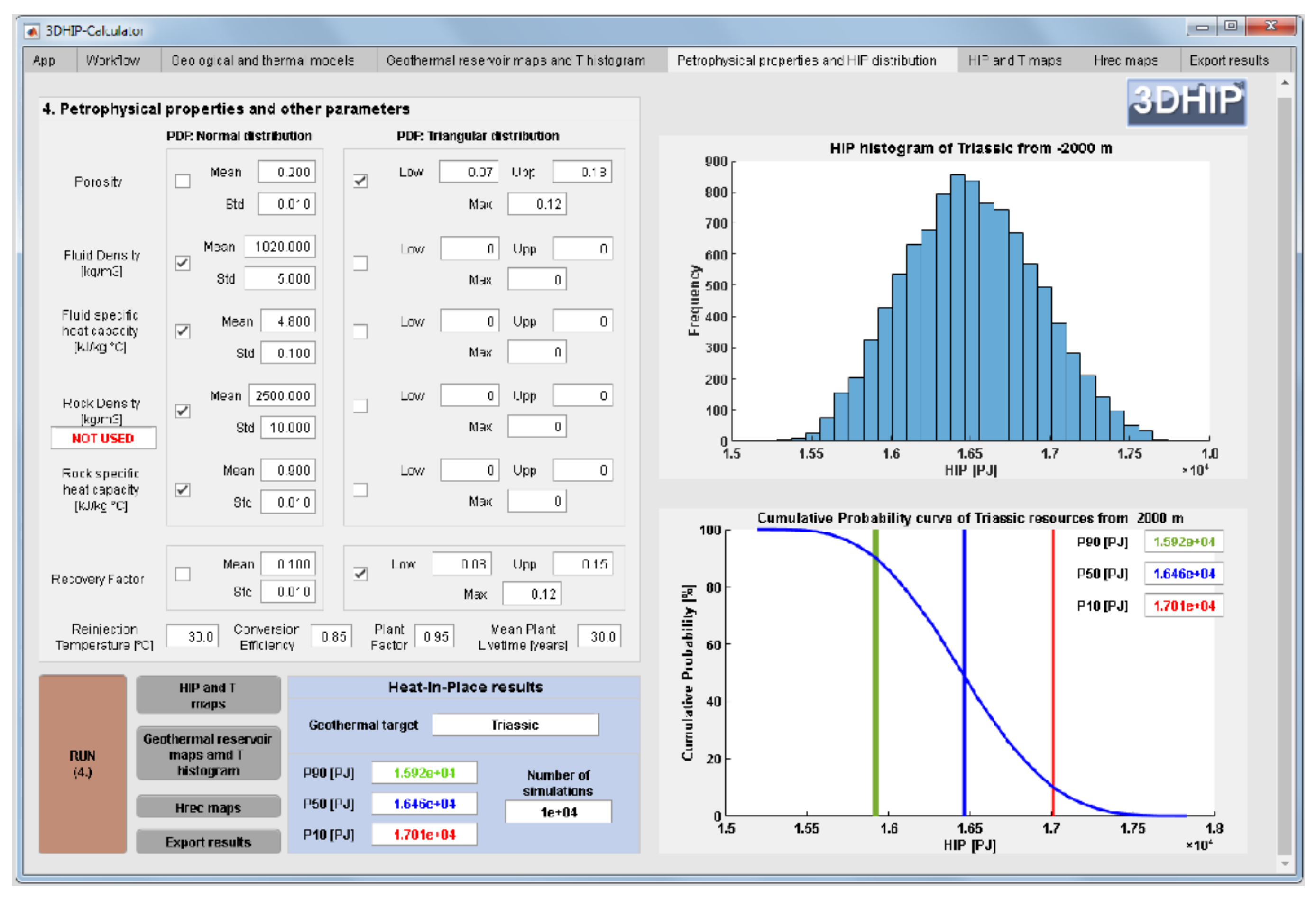
  • Generate a CDF for each voxel, from which a probability 10% (P10) (very low confidence of the estimation and high values), P50, and P90 (high confidence of the estimation and low values) are extracted. Furthermore, the mean and standard deviation are also calculated.
  • Generate a CDF for the entire investigated target (e.g., geological unit, reservoir, etc.) summing the voxel values, and the P10, P50, and P90 are calculated. This approach is only used for the HIP calculation and not for the Hrec one.
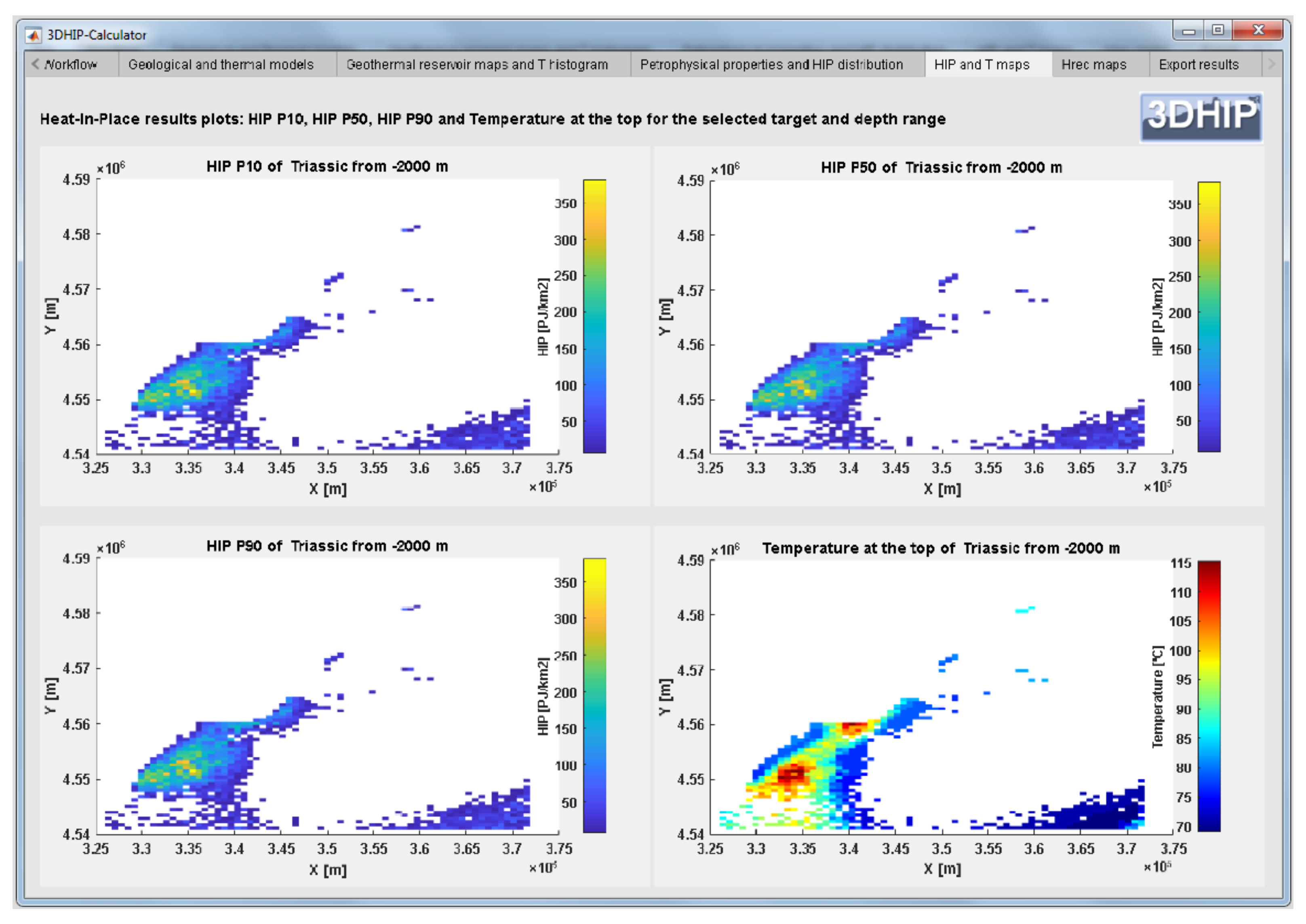
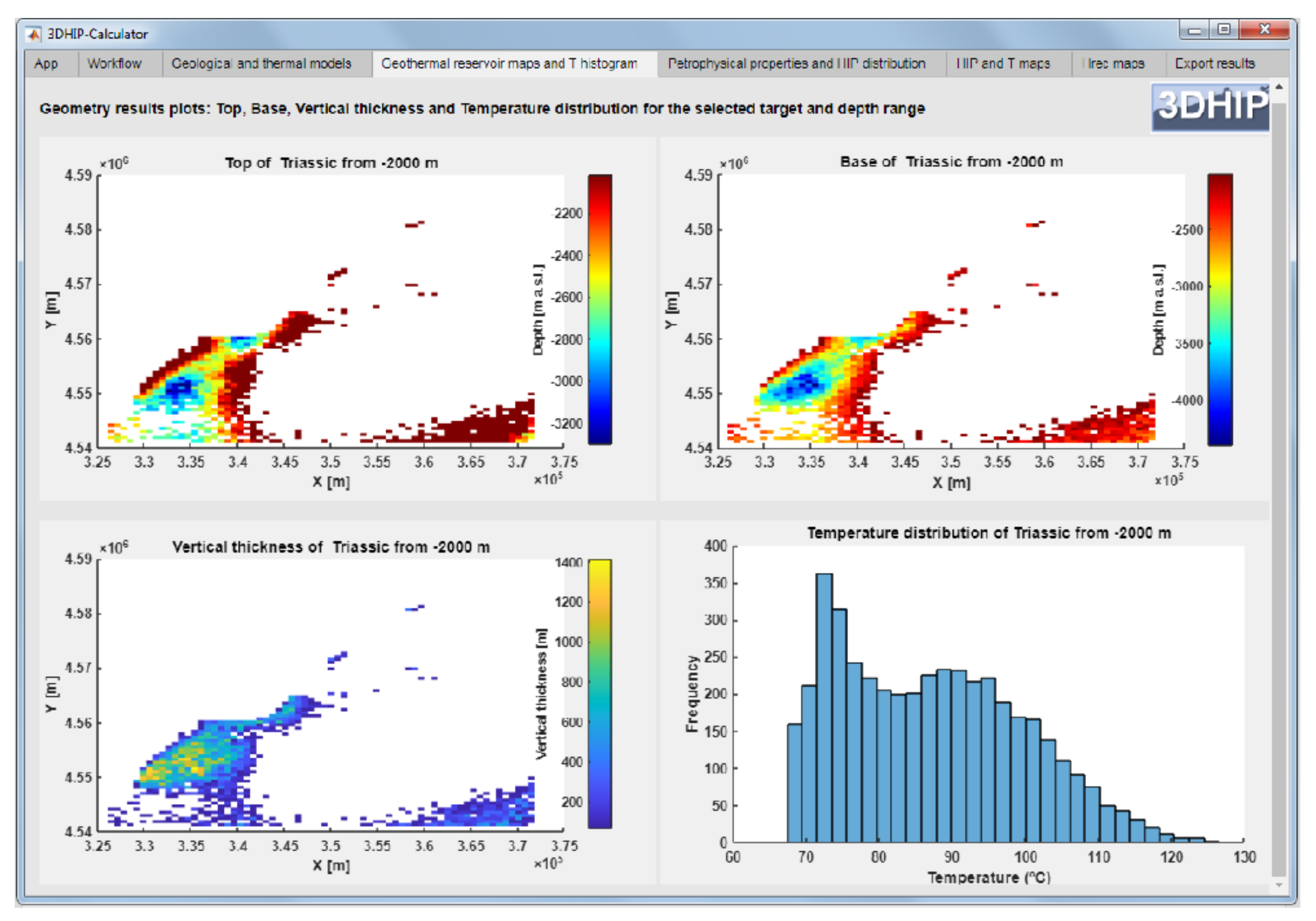
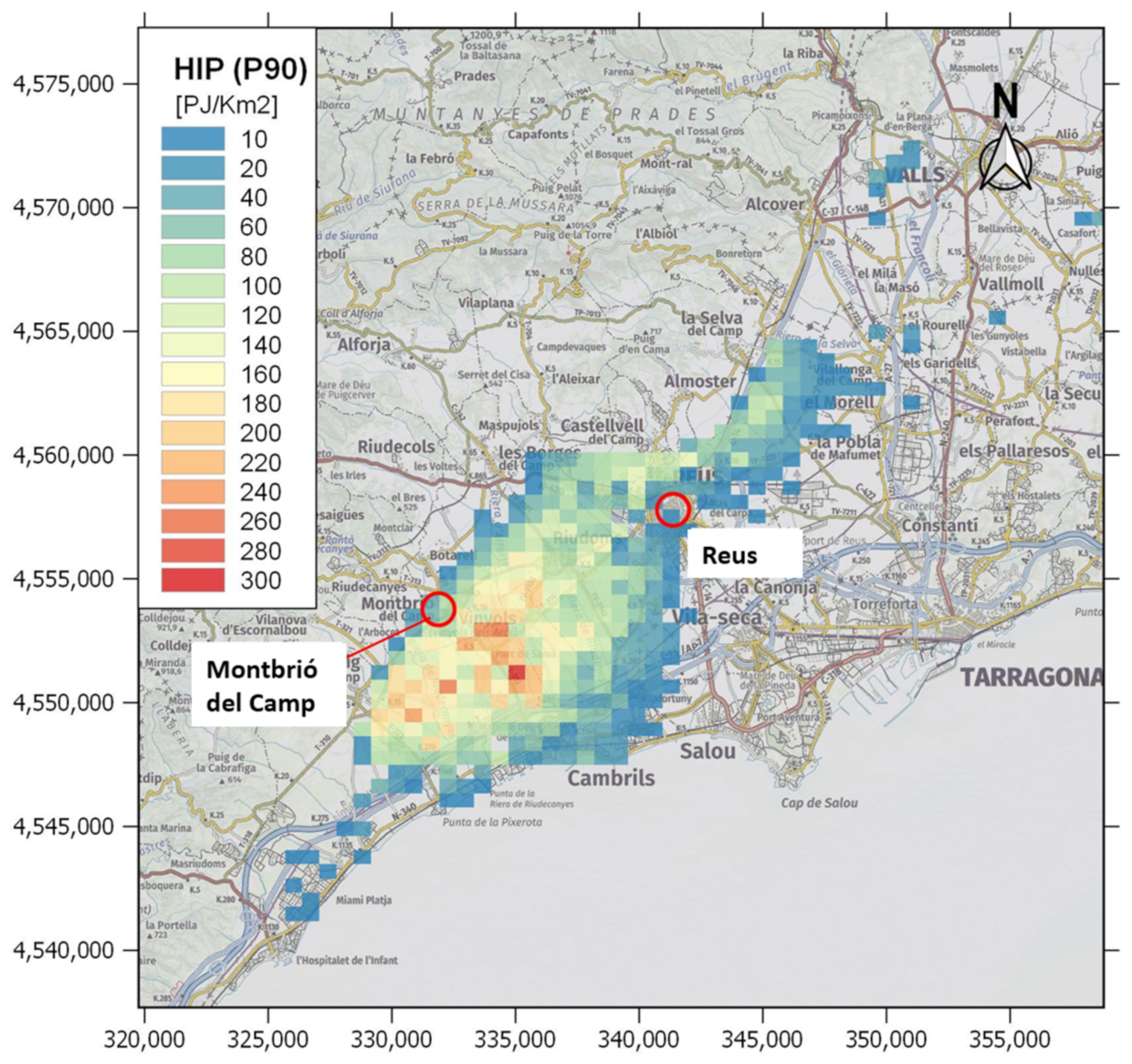
  • Generate 2D maps using the relationship between the vertical sum of the values calculated in each voxel with respect to the area occupied by the voxel (in km2). The P10, P50, and P90 of HIP and Hrec are then estimated.
  • The application allows exporting two ASCII files with all results for further post-processing and generates an automatic report that summarizes the input data and the main results.
One of these files is the 3D model with all the voxels of the selected target. Each output register for each voxel contains the initial data (X, Y, Z, and geology and thermal properties) plus the HIP (PJ) and Hrec (kW) calculations. The HIP and Hrec are expressed in terms of P10, P50, P90, mean, and standard deviation. This file can be exported again to 3D geological modeling software for subsequent post-processing, or to other environments, such as GIS suites (e.g., the results of this study are presented in maps using the free and open-source QGIS 3.16.1 ‘Hannover’ version), 3D visualization tools, or statistical packages such as R [33]. The second file is the 2D model with the vertical summation of the HIP (PJ) and Hrec (kW) values of each voxel and their coordinates (in this case only X and Y), which can also be used for further geospatial analysis in GIS for mapping. The values of HIP and Hrec are not divided by the voxel area, and they are expressed as they have been calculated, i.e., in P10, P50, and P90. Finally, the last file contains a brief report in text format that includes the data and parameters used for the simulation, as well as the main results obtained.

2.3.3. Modeling Scenarios Depending on Data Availability

The software can be used for different situations and contexts, depending on the availability of data. The optimal scenario is when both a 3DGM containing the distribution of petrophysical parameters (e.g., density, porosity) and a 3DTM with the same voxel structure that includes the temperature distribution with depth are available. An intermediate case would be when only a 3DGM is available and the temperature information of the study region is estimated using the mean geothermal gradient. In that case, the 3DHIP-Calculator can be run using a linear geothermal gradient instead of a thermal model. The worst scenario would be when the reservoir volume and temperature are roughly known, and the rest of the parameters need to be inferred. The 3DHIP-Calculator can also be used in these cases, although the uncertainty of the variables and resulting PDFs increase.

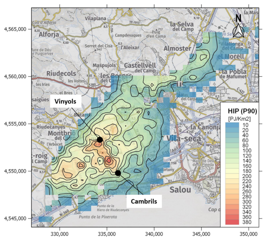
3. Example Case Study—The Reus-Valls Basin (NE, Spain)

This section demonstrates the use and capabilities of the 3DHIP-Calculator assessing the geothermal potential of the Reus-Valls Basin (RVB) based on the geological and thermal models presented by Herms et al. [34]. The Triassic and Jurassic units were selected as potential targets. As the main goal is to show the capabilities of the tool, the stratigraphic complexity of Triassic and Jurassic units was simplified in the model used for this analysis. The three scenarios described in the previous section are considered here to calculate the geothermal potential of the RVB. A fourth scenario that also includes the calculation of the recoverable heat is also considered here.

3.1. Geological Setting

The RVB is part of a set of SW–NE oriented extensional basins of the Catalan Coastal Ranges (Figure 4), which were formed during the Neogene rifting related to the opening of the Western Mediterranean and the Valencia Trough. The basin has a half-graben geometry strongly tilted towards its NW margin, where it is limited by the Camp Fault, which controls the basin depocenters [47]. This is an extensional NE-trending and SE-dipping basement fault [48] that was active from the early Miocene to the Quaternary. The fault separates the Prades-Llaberia and Miramar ranges (where the Mesozoic cover and the Paleozoic basement rocks crop out) and the Neogene sedimentary infill of the basin. These Neogene sediments reach a maximum thickness of about 2000 m near La Selva del Camp and Montbrió del Camp towns [47]. The Neogene sediments unconformably overlay the Mesozoic and the Paleozoic basement. Paleogene deposits are not preserved within the RVB, but such sediments lie unconformably on top of the Mesozoic succession in the Ebro Basin, NW of the study area.
There is no evidence of hydrothermal activity in the RVB except for the western limit of the basin, where there is a shallow hydrothermal aquifer controlled by W edge faults of the basin (called the ‘Camp Fault’) in the surroundings of the town of Montbrió del Camp. The hydrothermal aquifer shows an upward groundwater thermal flow of deep origin and a temperature of 81 °C at a 52 m depth. This fault-controlled hydrothermal aquifer is used nowadays by a thermal spa located within the town, exploiting its hot groundwaters.
Moreover, there is no evidence of magmatic activity, and it can be assumed that the main heat transport mechanism for the entire sedimentary basin at the regional scale is conduction. This is controlled by the thermal conductivity distribution of the lithologies that fill the basin and by the radiogenic heat production from the underlying granites. Therefore, the system can be classified as a conduction-dominated geothermal play in an intracratonic basin for the Mesozoic aquifers, which corresponds to a CD-1 of the catalog of geothermal play types based on geologic controls defined by Moeck [45,49] and CD-3 for the crystalline basement rocks.
Figure 4. Geological map with the delimitation of the Reus-Valls Basin (modified from [50]). Source of EU map: © EuroGeographics for the administrative boundaries, European Commission, Eurostat/GISCO.
Energies 14 07338 g004

3.2. The Potential Hot Deep Sedimentary Aquifers

The main deep aquifers acting as targets in the test case are in the Jurassic and Triassic limestones and sandstones. Currently, their deep geothermal energy potential is still untapped. It is well-known that these aquifers are geothermal reservoirs that have been exploited for a long time in other places of central and western Europe, such as the Malm limestones of the Molasse Basin in Germany [51], the Dogger limestones of the Paris Basin [52], and the Buntsandstein sandstones in northern Germany [53] and the Upper Rhine Graben [54].
The Jurassic sequence of the RVB is defined by a basal layer of brecciated dolostones followed by a carbonate interval constituted by limestones and sandy limestones with widespread dolomitization and karstification. In the old Reus-1 well (Figure 4), which was drilled for oil/gas exploration [55,56], these materials correspond to a 261 m thick unit of partially karstified dolostones, with an estimated porosity ranging between 11% and 21% and an average value of 16%, according to available data measured in the same facies of nearby offshore fields [56]. This unit was considered a possible reservoir target for an underground gas storage project in the 90’s due to its hydraulic properties.
The Middle Triassic corresponds to the Muschelkalk facies. These are defined from bottom to top by a basal interval of limestones and dolostones (Lower Muschelkalk), an intermediate interval of continental red fine sandstones, mudstones, and gypsum layers, and finally, an interlayered interval of limestones-dolostones and siltstone layers (Upper Muschelkalk). The total thickness of the unit is irregular in all the Catalan Coastal Ranges, and is about 359 m in the Reus-1 well. The basal dolostone (Lower Muschelkalk) is about 81 m thick in this well [55,56]. The main characteristics for inferring the reservoir porosity are the karstification of carbonates and the intense fracturing related to the Alpine exhumation and Neogene extension periods. Thus, the available data measured in nearby areas show values of primary porosity ranging between 7% and 12% (Ebro-1 and Fraga wells) [57], which can be considerably increased by secondary porosity. Finally, Buntsandstein facies (Lower Triassic) are composed of red detrital sediments formed by heteromeric conglomerates and fine sandstones, grading to mudstones at the top. The sedimentary sequence is constituted (from bottom to top) by a few meters of basal breccia, conglomerates, red sandstones, and a unit of interlayered siltstones with carbonate and evaporitic levels (Röt facies). Accordingly, the potential reservoir horizons that must be considered (in terms of host rock and fracture porosity) are the conglomerates and especially the sandstones of the lowest part of the sequence, with a total thickness range between 60 and 130 m in the Tarragona region [58]. The basal conglomerate has an irregular surface distribution and its porosity can be altered by its siltstone portion [59]. Moreover, the fluvial sandstones may have high porosity, as suggested by data from oil exploration wells (Ebro-1 and Ebro-2) in a nearby area, with average values of porosity ranging from 5.5% to 12.1%, with maximum values of 18% [57]. Attending to the range of measured porosities in the formations considered, a triangular distribution is consistent with the actual porosity pattern and is selected to be used for the reported examples (Table 1).
The 3DGM used for the RVB was built using the GeoModeller3D software (v4.0.8) after several iterative steps including additional geological and geophysical data [34]. First, a reference model was generated using a Digital Terrain Model 15 × 15 [60], the geological map 1:50.000 of the area [61], data from the surface-based 3D regional geological model of Catalunya [62], unpublished geological cross-sections, information from deep oil/gas borehole (Reus-1 well; BTH depth −2228 m and Z: +74.26 m a.s.l.), interpreted horizons from 2D seismic profiles, as well as complementary information from the borehole database of Catalonia [63]. To refine this model, a full gravity/magnetic litho-constrained stochastic geophysical inversion approach was carried out using a Bayesian inference scheme implemented in the geologic modeling package of GeoModeller3D based on Markov Chain Monte Carlo simulations [64,65]. The gravity and magnetic raw data used in the inversion process were obtained from the geophysical database of Catalonia [66]. The 3D inversion modeling was applied to fit the most probable 3DGM using a stochastic approach [34]. The resulted 3DGM honors all the available geological constraints (well data, density values, stratigraphic order, and surface geology), and the gravity and magnetic data.
The 3DTM was also prepared using GeoModeller3D, applying a forward modeling approach using the quasi-stochastic methodology called Parameter Sweep—an algorithm for heat resource uncertainty studies in steady-state. In this approach, we assumed that the main heat transport mechanism in the basin is thermal conduction. Dirichlet boundary conditions were assigned at the top and bottom of the model, with a pre-fixed temperature of 15 °C corresponding to the mean annual surface temperature on top, and 176 °C at a 7 km depth. The bottom temperature boundary condition of the model was set from a generalized 3D lithospheric scale steady-state conductive heat transfer model for the whole territory of Catalonia (NE, Spain), previously built with the software LitMod_3D, and assuming local isostasy [67]. This model considered three layers: two layers model the crust with constant values of radiogenic heat production and thermal conductivity, and a third layer models the upper mantle without radiogenic heat production and constant thermal conductivity. The LitMod_3D approach considers, among others, the effect of gravity, geoid, surface heat flow, and petrological and seismic data [68]. Several temperature layers were obtained from this model at the base of the crust and at 15, 7, and 3 km depths, with a corresponding temperature of 176 °C at a 7 km depth, which are currently published on the ICGC website [35].
Assuming an average ambient air temperature of 15 °C and a ground temperature of 176 °C at a 7 km depth, the resulting average thermal gradient is estimated at 23 °C/km considering the whole thickness of the model. However, if the calculation focuses on specific depths, the thermal gradient distribution can vary slightly with respect to this value due to the heterogeneous vertical distribution of thermal properties across the different lithologies. For example, the contrast between the lower thermal conductivity distribution in Neogene and Mesozoic sediments compared to the Paleozoic basement induces a local gradient of 28.3 °C/km, from the surface to the top of the Jurassic reservoir in the Reus-1 well. The petrophysical parameters, i.e., the mean value of thermal conductivity, the heat production rate, and their corresponding standard deviation, for each lithology were obtained from previous works and the literature [34]. As stated above, the 3DHIP-Calculator can be used in different contexts according to the available data and assumptions. To introduce the different options, different scenarios of data availability were considered.

3.2.1. Example 1: Using a Single-Voxel 1D Geological Model

The first case considered here corresponds to the worst-case scenario, where a voxel-based 3DGM is not available. In this case, we assume an idealized reservoir defined only by a single voxel, prepared in a simple way. We impose a fixed value for the reservoir whole volume and the parameters are defined according to the PDF. This approach can be useful to obtain a first-order estimation of the HIP when the geometry and temperature of the target reservoir and the model must be idealized as a single-voxel reservoir. This case is equivalent to those considered in the literature when using commercial applications such as @Risk (Palisade) or Crystal Ball (Oracle) [23,24,25], and by the ‘GPPeval’ Phyton-based stochastic library [27]. These software packages cannot consider the distributed 3D geometry of the reservoirs and therefore must assume the reservoir as a single volume.
Since the geological and thermal models are simplified to a single voxel, it is necessary to determine the total target reservoir volume in the calculations. The petrophysical and operational properties are introduced to indicate the corresponding triangular or normal distribution functions (Table 1). The results generated by the 3DHIP-Calculator tool are limited to the HIP histogram and the CDFs with the corresponding P10, P50, and P90 for the entire target (such as shown in Figure 5b for example 2).

3.2.2. Example 2: Using a 3DGM but Not a 3DTM

The second scenario assumes a 3DGM that contains only information of the lithology class of each voxel, but not of its petrophysical parameters (such as rock density, porosity, and thermal properties) or specific temperature data from a calibrated 3D thermal model to estimate the temperature distribution in all the voxels of the model. To address the thermal context in this scenario, a regional gradient is assumed using Equation (3). In this example, a regional geothermal gradient of 30 °C/km and a mean annual surface temperature of 15 °C are assumed. Thus, the depth–temperature profile directly results from Equation (3) (Figure 5a).
After uploading the 3DGM and providing an input value for the geothermal gradient (30 °C/km), a total of N = 10,000 realizations were carried out. This number of simulations is accepted by different authors as high enough for Monte Carlo evaluations [4,19,27,43]. For this example, we considered the Triassic unit as the geothermal target reservoir.
The selected depth range of the Triassic reservoir is indicated by two red lines in Figure 5. We selected the lower limit as the bottom of the model, while the upper depth corresponds to −2000 m a.s.l. The upper depth range was chosen as the limit where the reservoir temperature is >60 °C, a standard lower cut-off temperature for district heating stations [69]. The summary of petrophysical and operational properties, and their corresponding PDFs, are displayed in Table 1 and Figure 5b.
The values of the different parameters have been defined according to the available data, as well as from the scientific literature. The range of porosity values for the Buntsandstein and Muschelkalk units assumes a triangular PDF with porosity values of 7%, 12%, and 18% for the lowest, most probable, and highest values, respectively. Other parameters were obtained from the general literature, including the fluid density [70], fluid specific heat capacity [71], rock density [72], and rock specific heat capacity [73]. Considering the large uncertainty of the recovery factor (R), we used a triangular PDF with a lower value of 0.08, a most probable value of 0.12, and an upper value of 0.15, according to a conservative setting.
The results of the HIP and Hrec parameters can be displayed as histograms of their frequency and/or CDFs with P10, P50, and P90 values for the target reservoir (Figure 5b). Alternatively, the resulting HIP and Hrec values (P10, P50, and P90) can also be recalculated and displayed in 2D maps as the vertical summation of the calculated values assigned to each voxel divided by the voxel area in km2 (see Figure 6 for an example of HIP). In these maps, the voxels with a zero value were left without color. Finally, the results can be exported to GIS software packages for post-processing (e.g., QGIS), as shown in Figure 7, where an isoline map of the HIP_P90 is plotted to highlight the probability results.
The maximum geothermal potential in the study area (approximately 320–340 PJ/km2) is concentrated near the Vinyols town (Figure 7). This region coincides with the zone where the RVB is deeper and Triassic attains its higher thickness at the regional scale. This spatial distribution of the results shows not only an estimation of the geothermal potential but also reveals where the prospective zones for geothermal energy production are located within the RVB. This demonstrates the importance of using 3D georeferenced data as inputs, containing the spatial geological information in three dimensions.

3.2.3. Example 3: Using Both a 3DGM and a 3DTM

The third scenario corresponds to a case in which a 3DGM, which includes petrophysical data (e.g., density), and a 3DTM, with the temperature and its standard deviation for each voxel, are available. The number of simulations and the reservoir target are the same as those of the previous example. Figure 8 shows a graph of the temperature distribution against depth for all the voxels corresponding to the target reservoir. As the temperature distribution in depth is the result of a 3DTM, the temperature dispersion is lower than that of the previous example and less affected by topography. The reservoir top, base, vertical thickness, and temperature distribution are shown in Figure 9 for the selected target and depth range. A summary of the parameters and PDFs used in this scenario and the resulting HIP frequency and CDFs are displayed in Figure 10.
The HIP and Hrec results are displayed in a georeferenced map (Figure 11) to provide a background of geographical context, and this allows for further analysis. The highest values (260–300 PJ/km2) were observed southwest of the basin, concentrated around the town of Vinyols. However, in this scenario, the estimation of HIP values was sensibly lower than those of the previous example. This is because the 3DTM mean gradient is lower than that of the previous scenario.

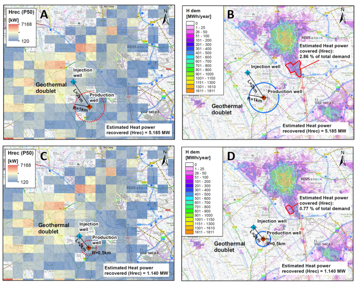
3.2.4. Example 4: The Use of the Recoverable Heat (Hrec) Values

The last scenario corresponds to a case in which the recoverable heat (Hrec) is also estimated. The results provide a first estimation of the percentage of the urban thermal demand that could be covered with the thermal energy recovered from a hypothetical geothermal doublet, where production and injection wells are typically separated from 1 to 2 km [72]. The Jurassic unit was considered as the target reservoir and the well locations were assumed to be next to the old Reus-1 oil well, where the Jurassic thickness is about 250 to 300 m from 1430 to 1700 m depth [54,55]. The example uses the same data assumption as that in example 3 (3DGM, which includes petrophysical data (e.g., density), and a 3DTM, with the temperature and its standard deviation for each voxel). For this case, the formation temperature oscillates between 55 and 65 °C and the rock porosity follows a normal distribution with a mean of 16% and a standard deviation of 5% [55]. Table 1 shows the other values used for the calculation.
Here, we compared the obtained Hrec with respect to the urban heat demand of the city of Reus (Figure 12). We compared the sum of the obtained Hrec for the different probabilities, Hrec_P10, Hrec_P50, and Hrec_90, under the influence radius of the hypothetical production deep well. Considering that the influence radius of the exploitation area in the reservoir has a value of half of the spacing between the injection and extraction wells (e.g., of up to 0.5 to 1 km), we obtained that the Hrec can range from 927 kW (P90 with 0.5 km of influence in the injection well) to 6.1 MW (P10 with 1 km of influence in the injection well). The heat demand density information was gathered from the Hotmaps EU project (https://www.hotmaps-project.eu (accessed on 15 October 2021)). The total heat energy demand obtained for the city of Reus was 391.05 GWh/year. Considering as a hypothesis that this demand concentrates during the colder part of the year (6 months) and with heaters working 12 h per day (2160 h/year), we can estimate the demand of thermal heat power capacity. In this case, the Hrec results suggested that a geothermal production well of a doublet in the Jurassic reservoir in this location could cover a range of 0.51% to 3.38% of the total heat demand of this city (Figure 12 and Table 2).
The Hrec results also suggest that the geothermal potential is much higher in the northwest of the Reus-1 well. This can be explained due to the fact that to the NW, the Jurassic formation lies deeper, up to 2000 m, and thus its temperature, following the 3DTM, oscillates between 70 and 80 °C. However, we considered a location close to the Reus-1 oil well to use its data.

4. Discussion and Conclusions

This paper describes a novel and freely available tool named the 3DHIP-Calculator, which is used to assess the deep geothermal energy potential of hot aquifers. The tool allows applying the HIP method to calculate the HIP and the Hrec of a target reservoir following a Monte Carlo stochastic approach, and using 3D geological and 3D thermal models as inputs. The HIP method [5] is widely known and used in geothermal energy studies. The tool can be used to generate probability maps, which are of particular importance during the preliminary assessment of geothermal resources, mainly at the regional scale. In this work, the operation and workflow of the 3DHIP-Calculator tool have been presented. Its use has been demonstrated through an example of an area identified with deep geothermal potential in Mesozoic aquifers located in the NE of the Iberian Peninsula (Reus-Valls Basin), and from considering four different conceptual scenarios based on the available data.
The 3DHIP-Calculator covers the need to have a standard and freely available tool for the whole geothermal community with which users can estimate the HIP using Monte Carlo simulations and where they can use their 3D models to assess their case studies. In this regard, the 3DHIP-Calculator is the only free tool that allows to carry out estimations of the geothermal potential assessment at the same time, either considering a homogeneous distribution of parameters (i.e., lumped parameter models) in the whole reservoir or including spatial variability of petrophysical properties through the considered reservoir (e.g., density and porosity). Moreover, the 3DHIP-Calculator is not regionally constrained and can be used to perform geothermal potential assessment exercises independently from where their data is. Additionally, the 3DHIP-Calculator simulations are not limited to a specific case study and the initial input data can change and incorporate data as these are refined or obtained through the reservoir characterization. The link between the 3DGM and 3DTM (examples 2 and 3), and the corresponding 3D geothermal potential assessment model (3DGPAM), represents an important step forward with respect to scenarios such as that of example 1, where the reservoir is represented as a single voxel and the geothermal potential results are limited to a single CDF with values of P10, P50, and P90 for the entire target reservoir, and where the option to include more data as the reservoir knowledge increases is truncated.
The results of the 3DGPAM can also again be exported back into 3D geological modeling software to carry out further steps of geothermal exploration of a specific project, or simply exported in 3D visualization software to plot the obtained results (e.g., the open-source, multi-platform data analysis and visualization application, such as ParaView).
The 3DHIP-Calculator is designed to assess and map geothermal resources at the regional scale. It bridges the gap between the first phases of field exploration and geological 3D modeling, and the necessary phase of quantification of the geothermal heat available in deep hot reservoirs, maintaining the uncertainty of the data. Therefore, it should be considered a complementary tool to the well-known open-source software DoubletCalc 2D [74], which allows calculating the hydraulic performance around geothermal doublets (producing well and injector) over time, and that is also based on stochastic simulations (Monte Carlo). Indeed, this analysis corresponds to a more advanced and detailed phase in the development of geothermal projects, considering, for example, that it is required for many grant applications related to specific geothermal projects in the Netherlands. The 3DHIP-Calculator is not designed to calculate the hydraulic performance of a doublet or to directly calculate the flow, temperature, and therefore the potential energy recovered from them, as other already available tools do for these purposes. However, it is able to make a first estimation from a hypothetical geothermal doublet, as shown in example 4.
The results obtained in the test case of the Reus-Valls Basin (NE, Spain) demonstrate how the 3DHIP-Calculator can satisfactorily evaluate and map the deep geothermal potential of reservoirs in a distributed manner from 3D models. In the presented test case study, the results reveal the existence of a high geothermal potential located between the villages of Vinyols and Cambrils (e.g., Figure 7). Although the exploration phase is in a preliminary stage, the results obtained considering the 3D modeling and the stochastic approach will allow progress in the decision-making process for the design of new exploratory campaigns, and thus increase the precision of the predictions. This modeling workflow has improved the estimates from previous studies based exclusively on a deterministic and a basin-wide aggregate approach [36,37,75].
The examples presented here demonstrate how geoscientists and engineers can use the 3DHIP-Calculator to easily evaluate the geothermal potential from their 3D geological models in a repeatable and systematic manner following a stochastic approach. The tool will help investors and research organizations determine the suitability of continuing to advance with new investments in pre-feasibility studies of future deep geothermal projects.

Author Contributions

Conceptualization, G.P.; Methodology, G.P., I.H. and A.G.; Software, G.P., I.H., A.G., M.C. and E.G.-R.; Resources, M.C. and G.A.; Writing—Original draft preparation, G.P.; Writing—Review and editing, I.H., A.G. and E.G.-R.; Visualization, M.C. and G.A.; Supervision, I.H., A.G. and E.G.-R. All authors have read and agreed to the published version of the manuscript.

Funding

G.P. was supported by Agència de Gestió d’Ajuts Universitaris i de Recerca (AGAUR) for Industry Doctorate Research 2016-DI-031 grant and by Institut Cartogràfic i Geològic de Catalunya (ICGC) through the MoU06092016ICGC-UAB and by the MoU11112019ICGC-UAB. E.G.-R. acknowledges the support of the Ramón y Cajal fellowship funded by the Spanish Ministry of Science, Innovation and Universities (RYC2018-026335-I and PID2020-118999GB-I00).

Institutional Review Board Statement

Not applicable.

Informed Consent Statement

Not applicable.

Data Availability Statement

The source code can be download from the following GitHub repository: https://github.com/OpenICGC/3DHIP-Calculator (accessed on 15 October 2021) mail for contact: [email protected]. The installation files, as well as the user manual in PDF format and some examples for testing the tool, can also be freely downloaded from the Deep geothermal energy web page of the Institut Cartogràfic i Geològic de Catalunya (ICGC) (under the Creative Commons license Attribution 4.0 International, CC BY 4.0).

Acknowledgments

The 3DHIP-Calculator software was developed during a PhD grant of the Industrial Doctorate programme sponsored by the AGAUR (Agència de Gestió d’Ajuts Universitaris i de Recerca) of the Government of Catalonia (reference number 2016-DI-031), and funded and maintained by the Institut Cartogràfic i Geològic de Catalunya (ICGC) under the project GeoEnergy of the CP-I (2014–2017), CP-II (2018), and CP-III (2019–2022). E.G.-R. acknowledges the Spanish Ministry of Science, Innovation and Universities for the “Ramón y Cajal” fellowship RYC2018-026335-I and research project PID2020-118999GB-I00. We thank the anonymous reviewers for their constructive comments and suggestions which led to a substantial improvement of the paper as well as all the researchers that has collaborated in this research.

Conflicts of Interest

The authors declare no conflict of interest.

References

  1. Bertani, R. Geothermal Power Generation in the World 2010–2015 Update Report. In Proceedings of the World Geothermal Congress 2015, Melbourne, Australia, 19–25 April 2015; pp. 19–25. [Google Scholar]
  2. Sigfússon, B.; Uihlein, A. 2015 JRC Geothermal Energy Status Report; EUR 27623 EN; Joint Research Center: Petten, The Netherlands, 2015; p. 59. [Google Scholar] [CrossRef]
  3. Van Wees, J.-D.; Boxem, T.; Angelino, L.; Dumas, P. A Prospective Study on the Geothermal Potential in the EU. GEOLEC Project; EC: Utrecht, The Netherlands, 2013; p. 97. [Google Scholar]
  4. Agemar, T.; Weber, J.; Moeck, I. Assessment and Public Reporting of Geothermal Resources in Germany: Review and Outlook. Energies 2018, 11, 332. [Google Scholar] [CrossRef] [Green Version]
  5. Muffler, P.; Cataldi, R. Methods for Regional Assessment of Geothermal Resources. Geothermics 1978, 7, 53–89. [Google Scholar] [CrossRef] [Green Version]
  6. Williams, C.F. Updated Methods for Estimating Recovery Factors for Geothermal Resources. In Proceedings of the Thirty-Second Workshop on Proceedings, Geothermal Reservoir Engineering, Stanford University, Stanford, CA, USA, 22 January 2007; p. 7. [Google Scholar]
  7. Williams, C.F.; Reed, M.J.; Mariner, R.H. A Review of Methods Applied by the U.S. Geological Survey in the Assessment of Identified Geothermal Resources; U.S. Geological Survey: Reston, VA, USA, 2008; p. 30.
  8. Garg, S.K.; Combs, J. Appropriate Use of USGS Volumetric “Heat in Place” Method and Monte Carlo Calculations. In Proceedings of the Thirty-Fourth Workshop on Geothermal Reservoir Engineering, Stanford University, Stanford, CA, USA, 1 February 2010; p. 7. [Google Scholar]
  9. Garg, S.K.; Combs, J. A Reexamination of USGS Volumetric “Heat in Place” Method. In Proceedings of the Thirty-Sixth Workshop on Geothermal Reservoir Engineering, Stanford University, Stanford, CA, USA, 31 February 2011; p. 5. [Google Scholar]
  10. Garg, S.K.; Combs, J. A Reformulation of USGS Volumetric “Heat in Place” Resource Estimation Method. Geothermics 2015, 55, 150–158. [Google Scholar] [CrossRef]
  11. Limberger, J.; Boxem, T.; Pluymaekers, M.; Bruhn, D.; Manzella, A.; Calcagno, P.; Beekman, F.; Cloetingh, S.; van Wees, J.-D. Geothermal Energy in Deep Aquifers: A Global Assessment of the Resource Base for Direct Heat Utilization. Renew. Sustain. Energy Rev. 2018, 82, 961–975. [Google Scholar] [CrossRef]
  12. Trumpy, E.; Botteghi, S.; Caiozzi, F.; Donato, A.; Gola, G.; Montanari, D.; Pluymaekers, M.P.D.; Santilano, A.; van Wees, J.D.; Manzella, A. Geothermal Potential Assessment for a Low Carbon Strategy: A New Systematic Approach Applied in Southern Italy. Energy 2016, 103, 167–181. [Google Scholar] [CrossRef]
  13. Miranda, M.M.; Raymond, J.; Dezayes, C. Uncertainty and Risk Evaluation of Deep Geothermal Energy Source for Heat Production and Electricity Generation in Remote Northern Regions. Energies 2020, 13, 4221. [Google Scholar] [CrossRef]
  14. Arango-Galván, C.; Prol-Ledesma, R.M.; Torres-Vera, M.A. Geothermal Prospects in the Baja California Peninsula. Geothermics 2015, 55, 39–57. [Google Scholar] [CrossRef] [Green Version]
  15. Pol-Ledesma, R.-M.; Carrillo-de la Cruz, J.-L.; Torres-Vera, M.-A.; Membrillo-Abad, A.-S.; Espinoza-Ojeda, O.-M. Heat Flow Map and Geothermal Resources in Mexico / Mapa de Flujo de Calor y Recursos Geotérmicos de México. Terra Digit. 2018. [Google Scholar] [CrossRef]
  16. Hurter, S.; Schellschmidt, R. Atlas of Geothermal Resources in Europe. Geothermics 2003, 32, 779–787. [Google Scholar] [CrossRef]
  17. Nathenson, M. Methodology of Determining the Uncertainty in the Accessible Geothermal Resource Base of Identified Hydrothermal Convec-Tion Systems; Open-File Report; U.S. Geological Survey: Menlo Park, CA, USA, 1978; p. 51.
  18. Rubinstein, R.Y.; Kroese, D.P. Simulation and the Monte Carlo Method, 3rd ed.; Wiley Series in Probability and Statistics; Wiley: Hoboken, NJ, USA, 2017; ISBN 978-1-118-63220-8. [Google Scholar]
  19. Shah, M.; Vaidya, D.; Sircar, A. Using Monte Carlo Simulation to Estimate Geothermal Resource in Dholera Geothermal Field, Gujarat, India. Multiscale Multidiscip. Model. Exp. Des. 2018, 1, 83–95. [Google Scholar] [CrossRef]
  20. Trota, A.; Ferreira, P.; Gomes, L.; Cabral, J.; Kallberg, P. Power Production Estimates from Geothermal Resources by Means of Small-Size Compact Climeon Heat Power Converters: Case Studies from Portugal (Sete Cidades, Azores and Longroiva Spa, Mainland). Energies 2019, 12, 2838. [Google Scholar] [CrossRef] [Green Version]
  21. Palisade Corporation. @Risk for Excel; Palisade Corporation: Ithaca, NY, USA, 2014. [Google Scholar]
  22. Oracle. Oracle Crystal Ball Spreadsheet Functions for Use in Microsoft Excel Models; Oracle: Austin, TX, USA, 2014. [Google Scholar]
  23. Arkan, S.; Parlaktuna, M. Resource Assessment of Balçova Geothermal Field. In Proceedings of the World Geothermal Congress 2005, Antalya, Turkey, 24–29 April 2005. [Google Scholar]
  24. Yang, F.; Liu, S.; Liu, J.; Pang, Z.; Zhou, D. Combined Monte Carlo Simulation and Geological Modeling for Geothermal Resource Assessment: A Case Study of the Xiongxian Geothermal Field, China. In Proceedings of the World Geothermal Congress 2015, Melbourne, Australia, 19–25 April 2015; pp. 19–25. [Google Scholar]
  25. Halcon, R.M.; Kaya, E.; Penarroyo, F. Resource Assessment Review of the Daklan Geothermal Prospect, Benguet, Philippines. In Proceedings of the World Geothermal Congress 2015, Melbourne, Australia, 19–25 April 2015; pp. 19–25. [Google Scholar]
  26. Barkaoui, A.-E.; Zarhloule, Y.; Varbanov, P.S.; Klemes, J.J. Geothermal Power Potential Assessment in North Eastern Morocco. Chem. Eng. Trans. 2017, 61, 1627–1632. [Google Scholar] [CrossRef]
  27. Pocasangre, C.; Fujimitsu, Y. Geothermics A Python-Based Stochastic Library for Assessing Geothermal Power Potential Using the Volumetric Method in a Liquid-Dominated Reservoir. Geothermics 2018, 76, 164–176. [Google Scholar] [CrossRef]
  28. Zhu, Z.; Lei, X.; Xu, N.; Shao, D.; Jiang, X.; Wu, X. Integration of 3D Geological Modeling and Geothermal Field Analysis for the Evaluation of Geothermal Reserves in the Northwest of Beijing Plain, China. Water 2020, 12, 638. [Google Scholar] [CrossRef] [Green Version]
  29. Calcagno, P.; Baujard, C.; Dagallier, A.; Guillou-Frottier, L.; Genter, A. Three-Dimensional Estimation of Geothermal Potential from Geological Field Data: The Limagne Geothermal Reservoir Case Study (France). In Proceedings of the Geothermal Resources Council GRC Annual Meeting, Reno, NV, USA, 4–7 October 2009; p. 326. [Google Scholar]
  30. Van Wees, J.-D.; Juez-Larre, J.; Bonte, D.; Mijnlieff, H.; Kronimus, A.; Gesse, S.; Obdam, A.; Verweij, H. ThermoGIS: An Integrated Web-Based Information System for Geothermal Exploration and Governmental Decision Support for Mature Oil and Gas Basins. In Proceedings of the World Geothermal Congress 2010, Bali, Indonesia, 25 April 2010; p. 7. [Google Scholar]
  31. Kramers, L.; van Wees, J.-D.; Pluymaekers, M.P.D.; Kronimus, A.; Boxem, T. Direct Heat Resource Assessment and Subsurface Information Systems for Geothermal Aquifers; the Dutch Perspective. Neth. J. Geosci. 2012, 91, 637–649. [Google Scholar] [CrossRef] [Green Version]
  32. Vrijlandt, M.A.W.; Struijk, E.L.M.; Brunner, L.G.; Veldkamp, J.G.; Witmans, N.; Maljers, D.; van Wees, J.D. ThermoGIS Update: A Renewed View on Geothermal Potential in the Netherlands. In Proceedings of the European Geothermal Congress 2019, The Hague, The Netherlands, 11 June 2019; p. 10. [Google Scholar]
  33. R Core Team. R: A Language and Environment for Statistical Computing; R Foundation for Statistical Computing: Vienna, Austria, 2013. [Google Scholar]
  34. Herms, I.; Piris, G.; Colomer, M.; Peigney, C.; Griera, A.; Ledo, J. 3D Numerical Modelling Combined with a Stochastic Approach in a MATLAB-Based Tool to Assess Deep Geothermal Potential in Catalonia: The Case Test Study of the Reus-Valls Basin. In Proceedings of the World Geothermal Congress 2020 + 1, Reykjavik, Iceland, 24–27 October 2021; p. 9. [Google Scholar]
  35. ICGC. Geothermal Atlas of Catalonia: Geoindex-Deep-Geothermal. 2020. Available online: https://www.icgc.cat/en/Public-Administration-and-Enterprises/Tools/Geoindex-viewers/Geoindex-Deep-geothermal-energy (accessed on 15 October 2021).
  36. Colmenar-Santos, A.; Folch-Calvo, M.; Rosales-Asensio, E.; Borge-Diez, D. The Geothermal Potential in Spain. Renew. Sustain. Energy Rev. 2016, 56, 865–886. [Google Scholar] [CrossRef]
  37. Arrizabalaga, I.; De Gregorio, M.; De Santiago, C.; Pérez, P. Geothermal Energy Use, Country Update for Spain. In Proceedings of the European Geothermal Congress 2019, The Hague, The Netherlands, 11 June 2019; p. 9. [Google Scholar]
  38. Beardsmore, G.R.; Rybach, L.; Blackwell, D.; Baron, C. A Protocol for Estimating and Mapping Global EGS Potential. Geotherm. Resour. Counc. Trans. 2010, 34, 301–312. [Google Scholar]
  39. Hurter, S.; Haenel, R. Atlas of Geothermal Resources in Europe; Official Publications of the European Communities, European Commission: Luxembourg, 2002. [Google Scholar]
  40. Lavigne, J. Les Resources Geothérmiques Françaises-Possibilités de Mise En Valeur. Ann. Mines 1977, 57–72. [Google Scholar]
  41. Williams, C.F. Development of Revised Techniques for Assessing Geothermal Resources. In Proceedings of the Twenty-Ninth Workshop on Geothermal Reservoir Engineering, Stanford University, Stanford, CA, USA, 26 January 2004; p. 5. [Google Scholar]
  42. Lund, J.W.; Boyd, T.L. Direct Utilization of Geothermal Energy 2015 Worldwide Review. Geothermics 2016, 60, 66–93. [Google Scholar] [CrossRef]
  43. Wang, Y.; Wang, L.; Bai, Y.; Wang, Z.; Hu, J.; Hu, D.; Wang, Y.; Hu, S. Assessment of Geothermal Resources in the North Jiangsu Basin, East China, Using Monte Carlo Simulation. Energies 2021, 14, 259. [Google Scholar] [CrossRef]
  44. MathWorks. MATLAB; The MathWorks, Inc.: Natick, MA, USA, 2019. [Google Scholar]
  45. Moeck, I.; Beardsmore, G.R. A New ‘Geothermal Play Type’ Catalog: Streamlining Exploration Decision Making. In Proceedings of the Thirty-Ninth Workshop on Geothermal Reservoir Engineering, Stanford University, Stanford, CA, USA, 24 February 2014; p. 8. [Google Scholar]
  46. De la Varga, M.; Schaaf, A.; Wellmann, F. GemPy 1.0: Open-Source Stochastic Geological Modeling and Inversion. Geosci. Model Dev. 2019, 12, 1–32. [Google Scholar] [CrossRef] [Green Version]
  47. Massana, E. L’activitat Neotectònica a Les Cadenes Costaneres Catalanes. Ph.D. Thesis, University of Barcelona, Barcelona, Spain, 1995. [Google Scholar]
  48. Cabrera, L.; Calvet, F. Onshore Neogene record in NE Spain: Vallès–Penedès and El Camp half-grabens (NW Mediterranean). In Tertiary Basins of Spain; Friend, P.F., Dabrio, C.J., Eds.; Cambridge University Press: Cambridge, UK, 1996; pp. 97–105. ISBN 978-0-521-46171-9. [Google Scholar]
  49. Moeck, I.S. Catalog of Geothermal Play Types Based on Geologic Controls. Renew. Sustain. Energy Rev. 2014, 37, 867–882. [Google Scholar] [CrossRef] [Green Version]
  50. ICGC. Base Geològica 1:50.000 de Catalunya. Available online: https://www.icgc.cat/en/Public-Administration-and-Enterprises/Downloads/Geological-and-geothematic-cartography/Geological-cartography/Geological-map-1-50-000 (accessed on 1 January 2021).
  51. Moeck, I.S.; Dussel, M.; Weber, J.; Schintgen, T.; Wolfgramm, M. Geothermal Play Typing in Germany, Case Study Molasse Basin: A Modern Concept to Categorise Geothermal Resources Related to Crustal Permeability. Neth. J. Geosci. 2019, 98, e14. [Google Scholar] [CrossRef] [Green Version]
  52. Lopez, S.; Hamm, V.; Le Brun, M.; Schaper, L.; Boissier, F.; Cotiche, C.; Giuglaris, E. 40 Years of Dogger Aquifer Management in Ile-de-France, Paris Basin, France. Geothermics 2010, 39, 339–356. [Google Scholar] [CrossRef]
  53. Blöcher, G.; Reinsch, T.; Henninges, J.; Milsch, H.; Regenspurg, S.; Kummerow, J.; Francke, H.; Kranz, S.; Saadat, A.; Zimmermann, G.; et al. Hydraulic History and Current State of the Deep Geothermal Reservoir Groß Schönebeck. Geothermics 2016, 63, 27–43. [Google Scholar] [CrossRef]
  54. Haffen, S.; Géraud, Y.; Diraison, M.; Dezayes, C.; Siffert, D.; Garcia, M. Temperature Gradient Anomalies in the Buntsandstein Sandstone Reservoir, Upper Rhine Graben, Soultz, France. In Proceedings of the Tu D203 09—76th EAGE Conference & Exhibition 2014, Amsterdam, The Netherlands, 16 June 2014. [Google Scholar]
  55. Zapatero, M.A.; Reyes, J.L.; Martínez, R.; Suárez, I.; Arenillas, A.; Perucha, M.A. Estudio Preliminar de las Formaciones Favorables para el Almacenamiento Subterráneo de CO2 en España; Instituto Geológico y Minero de España (IGME): Madrid, Spain, 2009; p. 135. [Google Scholar]
  56. AURENSA. Proyecto de Almacenamientos Subterraneos de Gas. Reus; Auxiliar de Recursos y Energía, S.A.: Madrid, Spain, 1996; p. 65. [Google Scholar]
  57. Campos, R.; Recreo, F.; Perucha, M.A. AGP de CO2: Selección de Formaciones Favorables en la Cuenca del Ebro; Informes Técnicos Ciemat; CIEMAT: Madrid, España, 2007; p. 124. [Google Scholar]
  58. Marzo, M. El Bundstandstein de los Catalánides: Estratigrafía y Procesos Sedimentarios. Ph.D. Thesis, Universitat de Barcelona, Barcelona, Spain, 1980. [Google Scholar]
  59. Zapatero, M.A.; Suárez, I.; Arenillas, A.; Marina, M.; Catalina, R.; Martínez-Orío, R. Proyecto Europeo GeoCapacity. Assessing European Capacity for Geological Storage of Carbon Dioxide; Instituto Geológico y Minero de España (IGME): Madrid, España, 2009; p. 162. [Google Scholar]
  60. ICGC. Model d’Elevacions Del Terreny de Catalunya 15 × 15 Metres (MET-15) v2.0. 2018. Available online: https://www.icgc.cat/Descarregues/Elevacions/Model-d-elevacions-del-terreny-de-15x15-m (accessed on 11 January 2021).
  61. ICGC. Mapa Geològic Comarcal de Catalunya. Full Del Baix Camp. 2006. Available online: https://www.icgc.cat/en/Public-Administration-and-Enterprises/Downloads/Geological-and-geothematic-cartography/Geological-cartography/Geological-map-1-50-000 (accessed on 11 January 2021).
  62. ICGC. Model 3D Geològic de Catalunya. 2013. Available online: https://www.icgc.cat/ca/Administracio-i-empresa/Descarregues/Cartografia-geologica-i-geotematica/Cartografia-geologica/Model-geologic-3D-de-Catalunya (accessed on 15 January 2020).
  63. ICGC. Base de Dades de Sondejos de Catalunya (BDSoC). 2015. Available online: https://www.icgc.cat/ca/Administracio-i-empresa/Eines/Visualitzadors-Geoindex/Geoindex-Prospeccions-geotecniques (accessed on 15 January 2020).
  64. Scott, S.W.; Covell, C.; Júlíusson, E.; Valfells, Á.; Newson, J.; Hrafnkelsson, B.; Pálsson, H.; Gudjónsdóttir, M. A Probabilistic Geologic Model of the Krafla Geothermal System Constrained by Gravimetric Data. Geotherm. Energy 2019, 7, 29. [Google Scholar] [CrossRef] [Green Version]
  65. Scott, S.; Covell, C.; Juliusson, E.; Valfells, Á.; Newson, J.; Hrafnkelsson, B.; Pálsson, H.; Gudjónsdóttir, M. A Probabilistic Geologic Model of the Krafla Geothermal System Based on Bayesian Inversion of Gravimetric Data. In Proceedings of the World Geothermal Congress 2020 + 1, Reykjavik, Iceland, 24–27 October 2021; p. 13. [Google Scholar]
  66. ICGC. Base de Dades Geofísica de Catalunya. 2013. Available online: https://www.icgc.cat/Administracio-i-empresa/Serveis/Geofisica-aplicada/Geoindex-Tecniques-geofisiques (accessed on 15 January 2020).
  67. Fullea, J.; Afonso, J.C.; Connolly, J.A.D.; Fernàndez, M.; García-Castellanos, D.; Zeyen, H. LitMod3D: An Interactive 3-D Software to Model the Thermal, Compositional, Density, Seismological, and Rheological Structure of the Lithosphere and Sublithospheric Upper Mantle: LITMOD3D-3-D Interactive code to model lithosphere. Geochem. Geophys. Geosyst. 2009, 10. [Google Scholar] [CrossRef] [Green Version]
  68. Carballo, A.; Fernández, M.; Jiménez-Munt, I. Corte Litosférico al Este de La Península Ibérica y Sus Márgenes. Modelización de Las Propiedades Físicas Del Manto Superior. Física Tierra 2011, 23, 131–147. [Google Scholar] [CrossRef] [Green Version]
  69. Agemar, T.; Weber, J.; Schulz, R. Deep Geothermal Energy Production in Germany. Energies 2014, 7, 4397–4416. [Google Scholar] [CrossRef]
  70. Oldenburg, C.M.; Rinaldi, A.P. Buoyancy Effects on Upward Brine Displacement Caused by CO2 Injection. Transp. Porous Media 2011, 87, 525–540. [Google Scholar] [CrossRef] [Green Version]
  71. Lukosevicius, V. Thermal Energy Production from Low Temperature Geothermal Brine—Technological Aspects and Energy Efficiency; ONU Geothermal Training Programme; Orkustofnum—National Energy Authority: Grensasvegur, Reykjavik, Iceland, 1993; p. 42.
  72. Ayala, C. Basement Characterisation and Cover Deformation of the Linking Zone (NE Spain) from 2.5D and 3D Geological and Geophysical Modelling. In Proceedings of the 8th EUREGEO, Barcelona, Spain, 15–17 June 2015; p. 23. [Google Scholar]
  73. Willems, C.J.L.; Nick, H.M. Towards Optimisation of Geothermal Heat Recovery: An Example from the West Netherlands Basin. Appl. Energy 2019, 247, 582–593. [Google Scholar] [CrossRef]
  74. Veldkamp, J.G.; Pluymaekers, M.P.D.; van Wees, J.-D. DoubletCalc 2D (v1.0) Manual; TNO 2015 R10216; TNO: Utrecht, The Netherlands, 2015. [Google Scholar]
  75. Arrizabalaga, I.; De Gregorio, M.; De Santiago, C.; García de la Noceda, C.; Pérez, P.; Urchueguía, J.F. Country Update for the Spanish Geothermal Sector. In Proceedings of the World Geothermal Congress 2020 + 1, Reykjavik, Iceland, 24–27 October 2021. [Google Scholar]
Figure 1. Screenshot of the main GUI window. The 3DHIP-Calculator is organized in eight tabs.
Energies 14 07338 g001
Figure 2. 3DHIP-Calculator workflow. It is divided into six main steps: (1) input values, (2) reservoir selection and parameters, (3) HIP and Hrec computation, (4) HIP probability curve, (5) HIP and Hrec probability maps, and (6) export data (modified from Herms et al., 2021 [34]).
Energies 14 07338 g002
Figure 3. Internal structure of the data files of the voxel-based geological (A) and thermal (B) models that the 3DHIP-Calculator needs to be imported.
Energies 14 07338 g003
Figure 5. (a) Depth–temperature distribution for the Triassic unit using a linear geothermal gradient (example 2). Each blue circle corresponds to a temperature value of each of the voxels that discretize the Triassic unit. The red lines indicate the fixed depth range for the HIP and Hrec calculations. (b) Petrophysical and operational properties, and the corresponding PDFs used for this example. On the right-side: the HIP histogram and its CDF (blue curve) with the P10 (red line), P50 (blue line), and P90 (green line) for the entire targeted reservoir.
Energies 14 07338 g005
Figure 6. 2D maps of the HIP results of the P10, P50, and P90, and the temperature distribution at the top of the Triassic units below the pre-fixed depth range. For the HIP parameters, the values were calculated as an integration over the depth range and normalized by the voxel area. Units are in PJ/km2 and °C, respectively.
Energies 14 07338 g006
Figure 7. The HIP with P90 for the Triassic unit (example 2). The map was plotted with constant contour lines (20 PJ/Km2) following the described second example (i.e., with a 3DGM but not a 3DTM).
Energies 14 07338 g007
Figure 8. Altitude with respect to the temperature distribution for the selected target in example 3 (Triassic unit). Each blue circle corresponds to a voxel temperature value within the target reservoir. The red lines indicate the depth range fixed for performing calculations.
Energies 14 07338 g008
Figure 9. 2D distribution map of the top, base, and vertical thickness of the Triassic unit. Maximum depth and thickness are observed SW of the basin. The temperature distribution for the Triassic unit is shown in the bottom right diagram.
Energies 14 07338 g009
Figure 10. Summary of the petrophysical and operational parameters and PDFs used in example 3. For this example, the 3D geological model includes a rock density value for each voxel, and for this reason, it was not stochastically simulated using a pre-scribed PDF. On the right: the HIP histogram and the HIP CDF’s results for the entire target reservoir (P10, P50, and P90).
Energies 14 07338 g010
Figure 11. 2D georeferenced map showing the HIP results obtained using example 3. The resulting HIP (P90) values are divided by the voxel area to express the results in PJ/km2. Only on-shore values are displayed.
Energies 14 07338 g011
Figure 12. Two geothermal doublet scenarios comparing the Hrec_P50 (AC) with the heat demand of the city of Reus (BD): the red polygon shows the covered area of the Reus total demand. (A,B) The injection and production wells are separated by 2 km and the radius of influence into the reservoir is considered to be 1 km. (C,D) The injection and production wells are separated by 1 km and the well influence radius into the reservoir is 0.5 km.
Energies 14 07338 g012
Table 1. Petrophysical and operational parameters used for the HIP and Hrec calculations in example 2 (Low and Upp correspond to the minimum and maximum temperature values assigned to the triangular distribution with lowest frequencies; Max—the value with the highest frequency; PDF—probability distribution function; SD—standard deviation).
PropertyUnitsPDFsValues
PetrophysicalPorosity -TriangularLow: 0.07, Max: 0.12, Upp: 0.18
Fluid Densitykg/m3NormalMean: 1020, SD: 5
Fluid specific heat capacitykJ/kg·°CNormalMean: 4.8, SD: 0.1
Rock densitykg/m3TriangularLow: 2450, Max: 2500, Upp: 2600
Rock specific heat capacitykJ/kg·°CNormalMean: 0.9, SD: 0.01
OperationalRecovery factor-TriangularMin: 0.08, Max: 0.12, Upp: 0.15
Reinjection temperature°C-30
Conversion efficiency--0.85
Plant factor--0.95
Mean plant lifetimeyears-30
Table 2. Estimated probable heat recovery capacity as a function of the influence radius for a hypothetical geothermal doublet well in the Jurassic reservoir close to the Reus-1 well.
Hrec—Recoverable Heat vs. Estimated R—Radius of InfluenceHrec P10 (kWt)Hrec P50 (kWt)Hrec P90 (kWt)
R = 0.5 km13371140927
R = 1 km612751854211
Publisher’s Note: MDPI stays neutral with regard to jurisdictional claims in published maps and institutional affiliations.

