Article

A Validation Study for RANS Based Modelling of Swirling Pulverized Fuel Flames

by
Ali Cemal Benim
1,*,
Cansu Deniz Canal
1,2 and
Yakup Erhan Boke
2
1
Center of Flow Simulation (CFS), Department of Mechanical and Process Engineering, Duesseldorf University of Applied Sciences, Muenstersr. 156, D-40476 Duesseldorf, Germany
2
Faculty of Mechanical Engineering, Istanbul Technical University, Istanbul 34437, Turkey
*
Author to whom correspondence should be addressed.
Energies 2021, 14(21), 7323; https://doi.org/10.3390/en14217323
Submission received: 28 September 2021 / Revised: 22 October 2021 / Accepted: 28 October 2021 / Published: 4 November 2021
(This article belongs to the Special Issue Computational Thermal, Energy, and Environmental Engineering)

Abstract

:
A swirling pulverized coal flame is computationally investigated. A Eulerian–Lagrangian formulation is used to describe the two-phase flow. Turbulence is modelled within a RANS (Reynolds averaged numerical simulation) framework. Four turbulence viscosity- (TV) based models, namely the standard k-ε model, realizable k-ε model, renormalization group theory k-ε model, and the shear stress transport k-ω model are used. In addition, a Reynolds stress transport model (RSM) is employed. The models are assessed by comparing the predicted velocity fields with the measurements of other authors. In terms of overall average values, the agreement of the predictions to the measurements is observed to be within the range 20–40%. A better performance of the RSM compared to the TV models is observed, with a nearly twice as better overall agreement to the experiments, particularly for the swirl velocity. In the second part of the investigation, the resolution of the discrete particle phase in modelling the turbulent particle dispersion (TPD) and particle size distribution (SD) is investigated. Using the discrete random walk model for the TPD, it is shown that even five random walks are sufficient for an accuracy that is quite high, with a less than 1% mean deviation from the solution obtained by thirty random walks. The approximation of the measured SD is determined by a continuous Rosin–Rammler distribution function, and inaccuracies that can occur in its subsequent discretization are demonstrated and discussed. An investigation on the resolution of the SD by discrete particle size classes (SC) indicates that 12 SC are required for an accuracy with a less than 1% mean deviation from the solution with 18 SC. Although these numbers may not necessarily be claimed to be sufficiently universal, they may serve as guidance, at least for SD with similar characteristics.

1. Introduction

Combustion has been used as the main process for power and heat generation from fossil fuels for many decades [1]. In recent years, renewable energy sources have been increasingly used to cover energy demands as well as to develop heat transfer enhancement techniques [2,3,4,5]. Parallel to this tendency towards renewable energies, combustion continues to play a significant role [6,7]. Combustion also plays a vital role in the field of renewable energies, especially due to the significance of biomass [8,9], which is not only because it is a renewable primary energy source but also due to its CO2 neutrality. For the utilization of biomass in utility boilers, it is rather common to co-fire pulverized coal and biomass. From this perspective, pulverized fuel combustion (of coal and/or biomass) is a technology that continues to claim an important part in the transformation of future energy system and deserves continuing attention.
The present investigation aims to contribute to the validation of mathematical models for the simulation of pulverized fuel combustion. Measurements obtained for a swirl burner with a thermal load of 60 kW at the test facility located at RWTH Aachen University are taken as the base of the experimental data.
Pulverized fuel combustion has been investigated by many researchers over several decades [10,11,12,13,14,15,16,17,18,19,20,21,22]. Comprehensive overviews on simulation procedures for the combustion of pulverized coal are provided in Epple et al. [23] and Hasse et al. [24]. Flames at the considered test facility (of RWTH Aachen) have also been computationally investigated previously by several researchers based on similar swirl burners of the same family. Essentially, two similarly constructed burners with two different thermal loads, i.e., 100 kW and 60 kW, have been computationally investigated before. Initial measurements for a 100 kWth pulverized coal flame were presented by Toporov et al. [25], where the k-ε model of turbulence was employed within a steady-state RANS (Reynolds averaged numerical simulation) formulation. Large eddy simulation (LES) and a RANS investigation of the same flame were performed by Chen and Ghoniem [26], where the standard and RNG k-ε model as well as the shear stress transport (SST) k-ω model were used as the RANS-based turbulence models. The same flame was analyzed using LES later on by Francetti et al. [27], who placed a focus on high-resolution LES modelling. The LES and RANS analysis of a further flame with 60 kWth at the same rig was presented by Sadiki et al. [28] for oxy-combustion. The realizable k-ε model was employed as the RANS model. A further numerical analysis of this 100 kWth flame was provided by Gaikwad et al. [29], who used a RANS approach for modelling turbulence using various two-equation turbulence models, namely the standard and RNG versions of the k-ε model and the SST k-ω model. Very recently, Nicolai et al. [30] presented an LES simulation of the 60 kWth flame (RWTH Aachen) in air and oxy-fuel atmospheres. Another recent LES investigation of a methane piloted pulverized coal swirl burner with 40 kWth (Technical University of Darmstadt) for air and oxy-combustion was presented by Wen et al. [31].
The purpose of the present study is to provide a further contribution to the validation studies using RANS-based modelling approaches on the basis of the present class of swirling pulverized fuel flames. Obviously, the LES approach has the potential of being more accurate than RANS models, as has already been demonstrated by the previous studies [28]. However, LES is still often found to be too costly for many engineering applications when it is applied professionally, fulfilling grid resolution requirements [32]. This is especially valid for large scale applications (such as utility boilers) and particulate flows with the necessity of transient particle tracking. Thus, the RANS approach can still be considered to be important for a wide range of engineering applications, and it constitutes the main focus of the present investigation.
In the above-mentioned studies [25,26,27,28,29], similar burners in the same test rig were analyzed using several RANS methods. Thus, the difference between the present contribution compared to previous work should be made clear. In the previous RANS studies on this category of flames, only turbulence viscosity-based turbulence models were investigated. The Reynolds stress model (RSM), which is known to be potentially more accurate for flows with a strongly non-isotropic turbulence structure, such as the present swirling flow [33], was not considered. In the present work, a broader range of turbulence viscosity-based turbulence models as well as RSM are considered within a “coherent” validation study. The coherence, i.e., the use of same methods for all other aspects of mathematical and numerical modelling, allows a more isolated comparison of this broad range of turbulence models.
A further question that is also addressed in the present study is related to the resolution of the particle phase in its discrete representation. The number of particles required to model the turbulent particle dispersion and particle size distribution are studied to suggest optimal values. This is important since the numbers of particles used in the modelling have a direct influence on the computational overhead. To the best of the authors’ knowledge, such a targeted study has not been performed before, not only for the type of flame being considered in the present study but also for pulverized fuel flames in general. Further, it should be mentioned that a RANS-based computational investigation of the presently considered 60 kWth flame for air combustion has not been presented before.

2. Modelling

The general-purpose computational fluid dynamics (CFD) code ANSYS Fluent 18.0 [34] was employed, which utilizes a finite volume method [35] of discretization.
The velocity–pressure coupling was conducted using the SIMPLEC pressure-correction procedure [36]. A body force-weighted interpolation was used for the pressure. For the discretization of the convective terms of all transport equations, the formally third-order accurate QUICK upwind scheme [37] was principally applied, with two exceptions: For the transport equations of the Reynolds stress components and for the SST model, the Power Law scheme [38] had to be used to obtain a steady-state converged solution for the RANS model. The gradient computation technique was least squares cell-based. Stabilization was achieved by having a standard cell face the slope limiter.
For the sake of completeness, an outline of the applied mathematical modelling is provided below. Detailed information beyond this overview can be found in various references [20,23,28,34,39,40].

2.1. Two-Phase Flow Modelling

Although the Eulerian–Eulerian formulation of the two-phase flow has also been successfully employed in pulverized coal combustion [41], the more commonly employed Eulerian–Lagrangian description [42] is adopted in the present study. The gas phase and particle phase equations were solved alternately, where the partial differential field equations were solved for the former and individual trajectories were integrated in time for the latter. The particle calculations were performed after each prescribed number (20 in the present calculations) of gaseous phase iterations. The phases are coupled by inter-phase mass, momentum, and energy transfer processes.

2.1.1. Eulerian Description of the Gas Phase

The density of the Newtonian gas mixture was calculated by assuming an ideal gas, neglecting the volume occupied by particles. A low Mach number flow was considered. Viscous dissipation and gravity were neglected. The molecular Lewis numbers of all of the gaseous species in the mixture were assumed to be unity [40]. The temperature dependence of the material properties was considered with fourth-order polynomials. In calculating the material properties, a turbulence interaction was omitted. Similarly, turbulent fluctuations were omitted when calculating the temperature-dependent terms of the radiation transport equation.
For the statistically steady turbulent flow of the gas mixture, the time-averaged mass, momentum, and energy conservation equations as well as the species transport equation are provided below. In those equations, the overbars and tildes that are usually used to indicate Reynolds- and Favre-averaged quantities [39] are omitted for simplicity. The variables that appear in convection terms, in multiplication with density, are to be interpreted as Favre- (density weighted) averages. The density and the remaining terms are to be understood as Reynolds-averaged quantities.
ρ u j x j = S m
ρ u j u i x j = p x i + x j { μ [ ( u i x j + u j x i ) 2 3 u k x k δ i j ] + τ i j t } + S u i
ρ u j h x j = x j [ μ Pr h x j + J h , j t ] + S h + S R
ρ u j Y k x j = x j [ μ S c Y k x j + J Y k , j t ] + Ω k + S Y k
In the above equations, ρ, μ, Pr, Sc, ui, p, h, and Yk denote the density, molecular viscosity, molecular Prandtl number, molecular Schmidt number, velocity vector, static pressure, standardized specific enthalpy, and the mass fraction of gas species k, respectively [40]. The terms τ i j t , J h , j t , and J Y k , j t denote the Reynolds stress tensor and the Reynolds flux vectors for enthalpy and species mass fraction, respectively. The source terms Sm, S u i , Sh, and S Y k take the interaction of the gas phase with the particle phase into account, while SR considers the radiation in the energy balance, and Ωk expresses the conversion of species k by the gas phase chemical reactions.

2.1.2. Lagrangian Description of the Particle Phase

Particle–particle interactions are omitted. The particle equations can thus be expressed based on a single particle with given initial properties. A particle cloud with variable properties (e.g., diameters) can then be represented by a number of classes (assuming homogeneity within each class). The results can subsequently be used to calculate the cumulative influence of the cloud on the gas phase after appropriate averaging, leading to the inter-phase source terms of the gas phase equations given above (not elaborated here). The accuracy depends on resolution, i.e., the number of classes considered. The variables appearing in the particle phase equations given below are obviously not averaged but are instead time-dependent quantities that can change in time in a Lagrangian sense, i.e., along the path of the particle.
Only the drag force is assumed to act on the particle. A spherical particle shape is assumed. The momentum balance of the particle can be expressed as
d m P u P , i d t = m P t r ( u i u P , i )
where mP, uP,i, and tr denote the particle mass, particle velocity vector, and the so-called particle relaxation time, respectively. The latter is defined as
t r = ρ P d 2 18 μ 24 C D Re P ; w i t h Re P = ρ d | u P , i u i | μ
while d, ρP, CD, and ReP denote the particle diameter, particle density, drag coefficient, and particle relative Reynolds number, respectively. The initial density of the dry coal particle is assumed to be 1400 kg/m3 in the present calculations. The drag coefficient CD (Equation (6)) is calculated using the correlations of Schiller and Naumann [43], which are based on ReP.
Assuming a uniform distribution of particle temperature (TP) within the particle, the energy balance for a particle can be written as
d m P c P T P d t = N u λ d A P ( T T P ) d m P d t H + A P ε P σ ( G 4 σ T P 4 )
In Equation (7) TP, cP, εP, AP, σ, and G represent the particle temperature, particle specific heat capacity, particle emissivity, particle surface area, the Stefan–Boltzmann constant, and incident radiation, respectively, while H denotes part of the heat that is released by the surface reaction that is absorbed by the particle. The particle-specific heat is assumed to be 1680 J/kgK, and the particle emissivity is taken to be 0.9. The variables Nu and λ denote the Nusselt number and gas thermal conductivity. The Nusselt number is calculated from the correlation of Ranz and Marshall [44,45] as function of the relative particle Reynolds number and the gas molecular Prandtl number.

2.2. Turbulence Modelling for the Gas Phase

The influence of the particle phase on gas turbulence is omitted. The RANS approach is employed to model the turbulent gas flow. Within this framework, different turbulence models are considered. These include turbulence viscosity- (TV) based models, as well as differential Reynolds stress model (RSM)

2.2.1. Turbulent Viscosity Models

Reynolds stresses are modelled by the Boussinesq hypothesis [39], which is based on the concept of turbulent viscosity (μt) as follows:
τ i j t = 2 μ t S i j 2 3 ( ρ k + μ t u k x k ) δ i j
where k and Sij, respectively, denote the turbulence kinetic energy and the strain rate tensor, with k = − τ i i t /2ρ, by definition. The shear rate tensor is defined as
S i j = 1 2 ( u i x j + u j x i ) ; w i t h S = S i j S i j
The Reynolds fluxes are modelled by the gradient-diffusion hypothesis
J h , j t = μ t Pr t h x j
J Y k , j t = μ t S c t Y k x j
where Prt and Sct denote the turbulent Prandtl number and turbulent Schmidt number, respectively, with the presently assumed values Prt = 0.85 and Sct = 0.7 (these numbers are defined as variables in RNG-KE, which attain the value of 0.718 for a high-turbulence Reynolds number).
Four TV-based two-equation models, namely the standard k-ε model [46] (S-KE), the realizable k-ε model [47] (R-KE), the renormalization group theory k-ε model [48] (RNG-KE), and the shear stress transport k-ω model [49] (SST) are considered. The variables ε and ω denote the turbulence energy dissipation rate and the specific dissipation rate, respectively. For simplicity, the high-turbulence Reynolds number (Ret) versions of the models are considered when outlining the model equations (Ret = μt/μ), which is also realistic for the prevailing high Reynolds number flow (with the exception of local regions, such as those near walls, which are, however, not addressed here for simplicity). The near-wall turbulence is modelled by the standard wall-functions approach [46].
The turbulent viscosity is obtained from
μ t = ρ C μ k 2 ε ( k ε mod e l s )
μ t = ρ C μ k ω ( S S T mod e l )
where the differences in the considered TV models can be expressed through different definitions of the model coefficient Cμ, which are summarized in Table 1.
The modelled transport equation for the turbulence kinetic energy can be expressed as follows (for SST, substitute ε = Cμωk in the last term)
ρ u j k x j = x j [ ( μ + μ t σ k ) k x j ] + G k ρ F k ε
where σk and Gk denote the turbulent Prandtl number for k and the generation of turbulence kinetic energy by the mean velocity gradients, respectively. The generation term is calculated as
G k = μ t S 2
while the σk and Fk for different models are provided in Table 2.
The modelled transport equations for ε (k-ε models) and for ω (relevant for the SST model) can be expressed as
ρ u j ε x j = x j [ ( μ + μ t σ ε ) ε x j ] + F 1 ε F 2 ε 2
ρ u j ω x j = x j [ ( μ + μ t σ ω ) ω x j ] + ρ ( F 1 μ t G k F 2 ω 2 + F 3 ω k x j ω x j )
where the functions F1, F2, and F3 are summarized in Table 3.

2.2.2. Differential Reynolds Stress Model (RSM)

In the differential Reynolds stress model [39], instead of utilizing the Boussinesq hypotheses, the Reynolds stresses are obtained from the solution of their modelled transport equations, which are given below
u k τ i j t x k = x k [ ( μ + μ t σ R S M ) τ i j t x k ] + ( τ i k t u j x k + τ j k t u i x k ) + 2 3 ρ ε δ i j ρ θ i j
where σRSM is taken to be equal to 0.82, and θij denotes the so-called pressure–strain term. The latter is modelled as a complex function of Reynolds stresses, rate of strain, and rate of rotation tensors. Presently, the model by Speziale et al. [50] is used for its modelling. The model needs the ε field to be closed, which is obtained from the solution of the modelled transport equation for ε (Equation (16)), with the constants of S-KE. Along with the wall-functions method [46], the wall boundary conditions for the Reynolds stresses are obtained by solving a transport equation for k, which is principally equivalent to the one depicted above for S-KE. In using RSM, the Reynolds fluxes that are needed to calculate heat and mass transfer are still obtained based on the gradient-diffusion hypotheses (Equations (10) and (11)).

2.3. Turbulence Modelling for the Particle Phase

The effect of gas turbulence on the particle motion is modelled by the so-called “discrete random walk” model [51]. Here, in calculating the particle path (Equation (5)), an “instantaneous” gas velocity is used to model the turbulent fluctuations in the gas phase. To this purpose, a “fluctuational value” is added to the averaged gas velocity temporarily. Using the TV-based models, the fluctuating velocity vector ui′ is obtained from k by assuming isotropy, and while using the RSM, the ui′ vector is obtained from the diagonal terms of the Reynolds stress tensor
u i = ζ 2 3 k ( T V mod e l s ) ; u i = ζ 1 ρ | τ i i t | ( R S M )
where ζ denotes a normally distributed random number.
The particle is assumed to interact with the gas-phase eddy over a time scale tP. When this time is reached, a new set of instantaneous velocity components are calculated by updating the value of ζ. This time scale is calculated as the minimum of the eddy life time and particle eddy crossing time, which is obtained from
t P = min { ξ k ε ; t r ln [ 1 ( k 3 / 2 / ε 4 ρ P d / 3 ρ C D ) ] }
In the above equation, the model constant ξ takes the value 0.6 for the RSM and 0.3 for the remaining turbulence models. Compared to the SST model, ε = 0.09 kω should be substituted in the above equation. Due to the random nature of the model, a sufficiently large number of trajectories need to be calculated (trials) to obtain sufficiently smooth and steady mean values.

2.4. Radiation Modelling

The radiative heat transfer is modelled by the P1 method [52], the transport equation of which is provided below
x j { [ 1 3 ( a + a P + s P ) ] G x j } = [ a + a P ] G 4 π [ a σ T 4 π + E p ]
where G, a, aP, sP, and EP denote the incident radiation, gas absorption coefficient and equivalent particle absorption coefficient, scattering coefficient, and emission, respectively. Assuming an equivalent path length for the domain, the absorption coefficient of the gas mixture can be calculated using the weighted sum of gray gases model [53]. The equivalent particle absorption and scattering coefficients and emission are obtained by the adequate averaging of the Lagrangian particle data, which are based on the given particle emissivity, geometry, temperature, and scattering factor fS [34]. The latter is assumed to be 0.9. The walls are assumed to reflect diffusely, where the detailed formulation of the boundary conditions can be found elsewhere [34,52].
The radiation source term of the gas phase energy equation (Equation (3)) is then calculated from
S R = 4 π ( a σ T 4 π + E P ) + ( a + a P ) G

2.5. Combustion Modelling

The fuel particle experiences an evaporation and pyrolysis with increasing temperature. The residual char burns via heterogeneous reactions, as the combustible volatile matter reacts homogeneously in the gas phase.

2.5.1. Pyrolysis

Following Badzioch and Hawskley [54], the conversion rate of the raw solid fuel through pyrolysis is expressed by a single-rate first-order expression as:
d m P d t = k P Y [ m P ( 1 f V M , 0 ) ( 1 f W , 0 ) m P , 0 ]
where fVM,0 and fW,0 denote the volatile matter and water mass fractions originally present in the particle, respectively, while mP,0 is the initial particle mass. The term kPY denotes the pyrolysis rate coefficient, which is expressed by an Arrhenius expression as follows:
k P Y = A P Y exp ( E P Y / T P )
with the corresponding pre-exponential factor APY and activation energy EPY that are to be empirically determined. The individual gas constant is denoted by . During pyrolysis, the swelling of the particles can be considered through a swelling coefficient [34]. This is chosen to be 1.4, implying an increase of particle diameter of up to 40% during pyrolysis. The combustible volatile matter is represented by a CαHβOγNη molecule and by assuming a molar mass of 30 kg/kmol, where α, β, γ, and η depend on the elementary analysis of the fuel.
The pyrolysis rate has a quite substantial influence in the prediction of pulverized fuel combustion. Since it depends strongly on the type of the fuel, and since its accurate determination is not very straightforward, an uncertainty quite often remains in this respect. In the single-rate pyrolysis process assumed in the present work, which is characterized by an Arrhenius rate expression, the pre-exponential factor and the activation energy are required as input. In the present study, values that were employed in previous numerical simulations by other authors are used [28,29], with the same type of coal being used as well. These are APY = 2.0·105 1/s, EPY = 4.8·107 J/kmol.

2.5.2. Char Oxidation

The modelling concept suggested by Field et al. [55] and Baum and Street [56] is adopted. The char conversion rate is calculated by considering a combined limiting effect of the chemical kinetics rate coefficient (kC) and the oxygen diffusion rate coefficient (kD), which can be expressed as:
d m P d t = A P k C k D k C + k D p O 2
where AP and pO2 represent the particle surface area and oxygen partial pressure, respectively. The diffusional and kinetical rate coefficients are calculated from:
k D = D 0 d [ ( T P + T ) / 2 ] 0.75
k C = A C exp ( E C / T P )
with the coefficients D0, AC, and EC, which are to be empirically determined. For them, the quite commonly used values from [57] are employed in the present calculations, resulting in values of D0 = 5·10−12, AC = 0.002, and EC = 7.9·107 J/kmol. During char oxidation, the particle size is assumed to stay constant, and the density is allowed to decrease.

2.5.3. Gas Phase Reactions

The effect of the turbulence–chemistry interaction is considered by a rather simple approach. The time-averaged conversion rate of a gas species k in a reaction r is assumed to be limited by the smaller of the kinetic and the fine-scale mixing rates. The resultant species conversion rate (Equation (4)) can be expressed as
Ω k = M m k r min ( R k , C , r , R k , E D M , r )
where the subscript r indicates the involved reaction and where Mmk, Rk,C,r, and Rk,EDM,r denote the species molar mass, the molar kinetics conversion rate, and molar fine-scale mixing conversion rate in the reaction r, respectively. Assuming irreversible reactions, the chemical molar conversion rate of species k in reaction r is obtained from [40]
R k , C , r = ν k , r k r s [ ( ρ / M m s ) Y s , r ] γ s , r
where index s counts over the reactant gas species of reaction r and where νK,r, kr, and γs,r denote the stoichiometric coefficient, kinetics rate coefficient, and the rate exponent, respectively. The rate coefficient kr is calculated from the Arrhenius kinetics as shown below, with Ar and Er denoting the corresponding pre-exponential factor and activation energy.
k r = A r exp ( E r / T )
The fine-scale mixing rate is modelled by the eddy dissipation model (EDM) by Magnussen and Hjertager [58]. Here, the molar conversion rate of a species k in a reaction r is limited by fine-scale mixing, which is calculated from
R k , E D M , r = ν k , r A ρ ε k min [ min ( Y r e a c ν r e a c M m r e a c ) , B Y p r o d ν p r o d M m p r o d ]
which is based on the mass fractions, stoichiometric coefficients, and molar masses of the reactant (reac) and product (prod) species of the considered reaction r. The coefficients A and B are the model constants. For them, the originally proposed values are used in the present calculations, i.e., A = 4.0, B = 0.5 [58].
In the presently assumed chemical mechanism, the combustion of the volatile matter occurs via a global reaction scheme comprising two irreversible reactions. In the first reaction, the volatile matter is assumed to react with CO and H2O. The second reaction is the oxidation of CO to CO2. The presently used rate constants for the chemical kinetics [34,59,60] are A1 = 2.119·1011, E1 = 2.027·108 J/kmol, γVM,1 = 0.2, and γO2,1 = 1.3 for the first reaction (volatiles oxidation), and A2 = 2.239·1012, E2 = 1.7·108 J/kmol, γCO,2 = 1, and γO2,2 = 0.25 for the second reaction (CO burn out).
The calculation of the time-averaged species conversion rates via Equation (28) based on EDM is a quite simplistic approach for the consideration of the turbulence–chemistry interaction. Among the more sophisticated approaches, flamelet-based methods, which have a longer tradition in certain applications such as gas turbine combustion [6], offer an attractive alternative since they can incorporate detailed chemistry at comparably low computational costs and can provide better accuracy (especially for species governed by fast reactions). Recently, the flamelet method has been extended to pulverized coal, and flamelet-based approaches are being used to simulate pulverized coal flames [30,31]. However, since the main focus of the present work has been the turbulence modelling, i.e., the relative assessment of turbulence models, and the discretization of the particle phase, the present EDM-based combustion model was found to be sufficient.

3. Test Case and Fuel Specific Definitions and Modelling

As already discussed above, the presently analyzed flames were obtained and measured at a test rig of RWTH Aachen University. A turbulent swirling flame of pulverized coal with a thermal load of 60 kW was considered as the test case.
At this stage, it should be stated that swirl application is very common in pulverized coal burners. A rotational motion is imparted to the burner flow, which is termed as a swirl. The rotational velocity component around the burner axis is the so-called swirl velocity. If a cylindrical coordinate system is used in an axi-symmetric formulation, which is presently the case, the swirl velocity is identical to the tangential (circumferential) velocity component in the cylindrical coordinate system.
The oxidizing medium is air, whereas the oxygen content of the primary stream deviates slightly from the atmospheric air, as shown below. The measurements on this type of flame were published in Zabrodiec et al. [61]. Illustrations of the experimental rig and the swirl burner are provided in Figure 1.
The operating conditions for the flame [61] are provided in Table 4.
The burner injections imply a locally fuel-rich mixture with a local equivalence ratio of nearly 1.3, whereas the global equivalence ratio is about 0.8. A swirling flame is generated by swirling the secondary gas stream with a geometric swirl number of 0.95 [61].
The ultimate and proximate analyses [61] of the used coal are provided in Table 5. Note that the sulphur content is omitted in the present simulations.
The measured particle size distribution for this coal was provided by Hees et al. [62].

Discrete Representation of the Particle Phase

In the presently applied Lagrangian formulation of the particle phase, the measured particle size distribution is applied exactly. The diameter values given in the experimentally provided distribution [62] define the borders between the individual size classes. The representative particle diameter in each size class is assumed to be given by the arithmetic average of the bordering sieve diameters (dS). The percentage volume contained in each size class is given by the difference in the amounts passing through the neighbouring sieve sizes. Assuming the minimum particle size to be 1 μm, the resulting particle size distribution, which has 18 particle size classes (N = 18), is provided in Table 6, where the diameters (d) of the size classes and the fractions of the particle mass within each size class (Δm) are presented.
To model the turbulent particle dispersion, 20 trials are applied for each size class. The sensitivity of the results to the number of size classes and number of trials will be investigated in the second part of the paper, subsequent to the comparison of the predictions of the measurements.

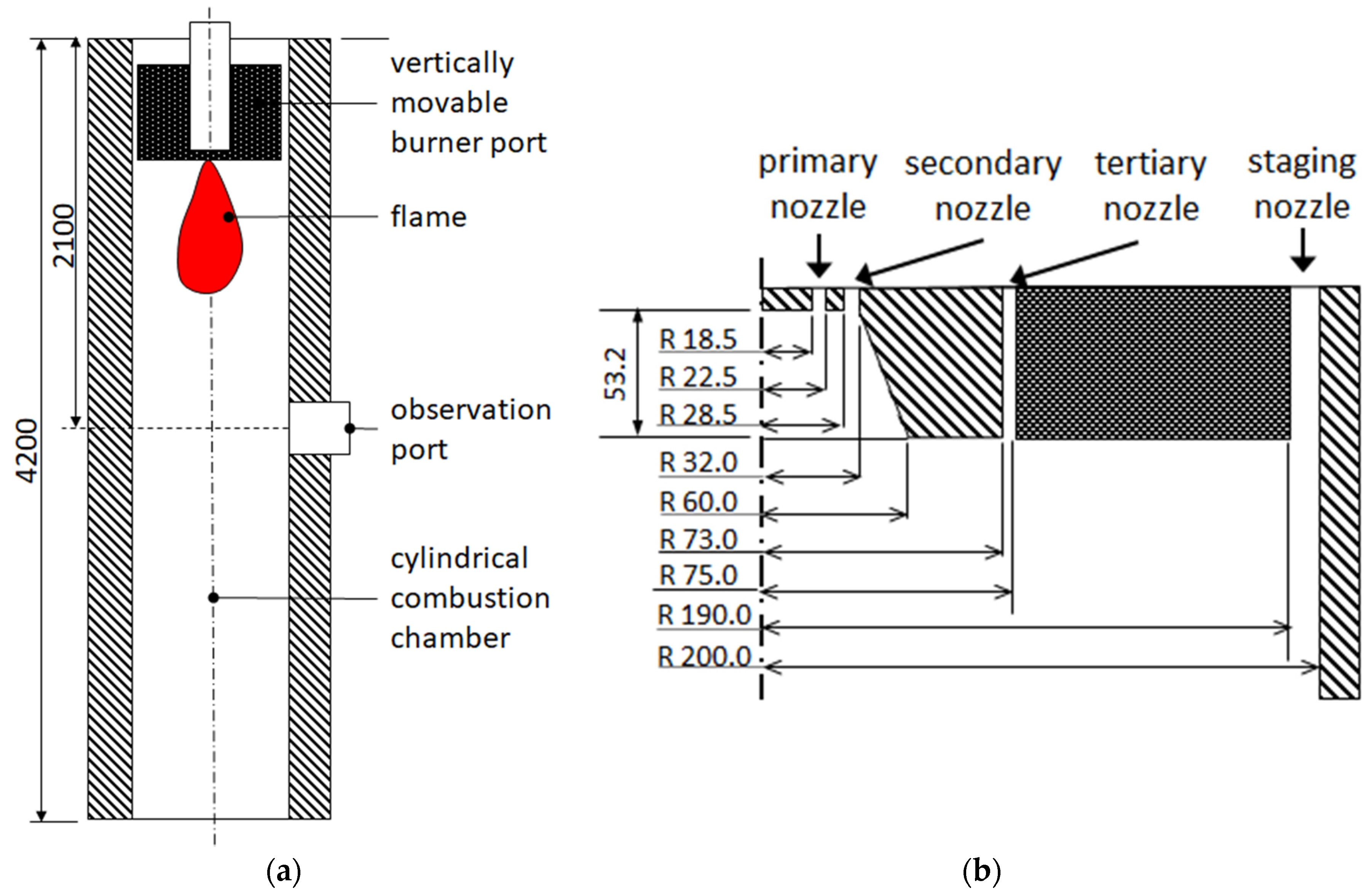
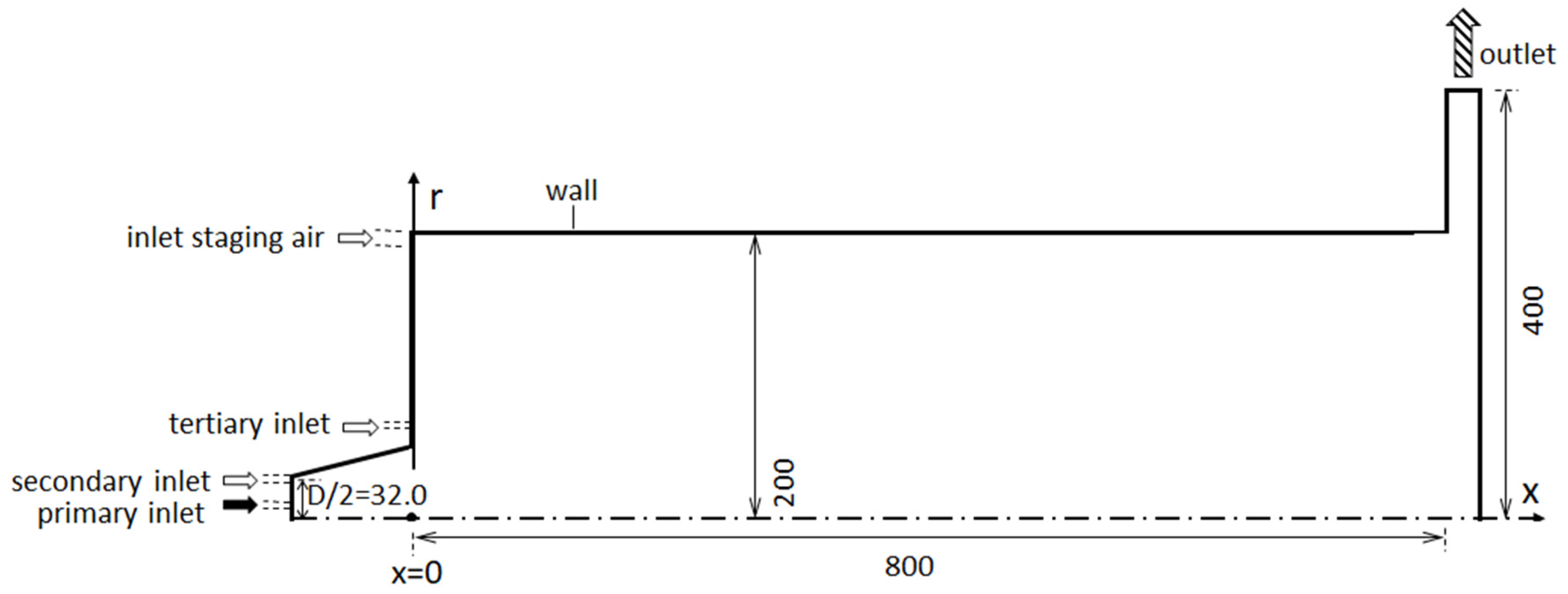
4. Solution Domain, Boundary Conditions
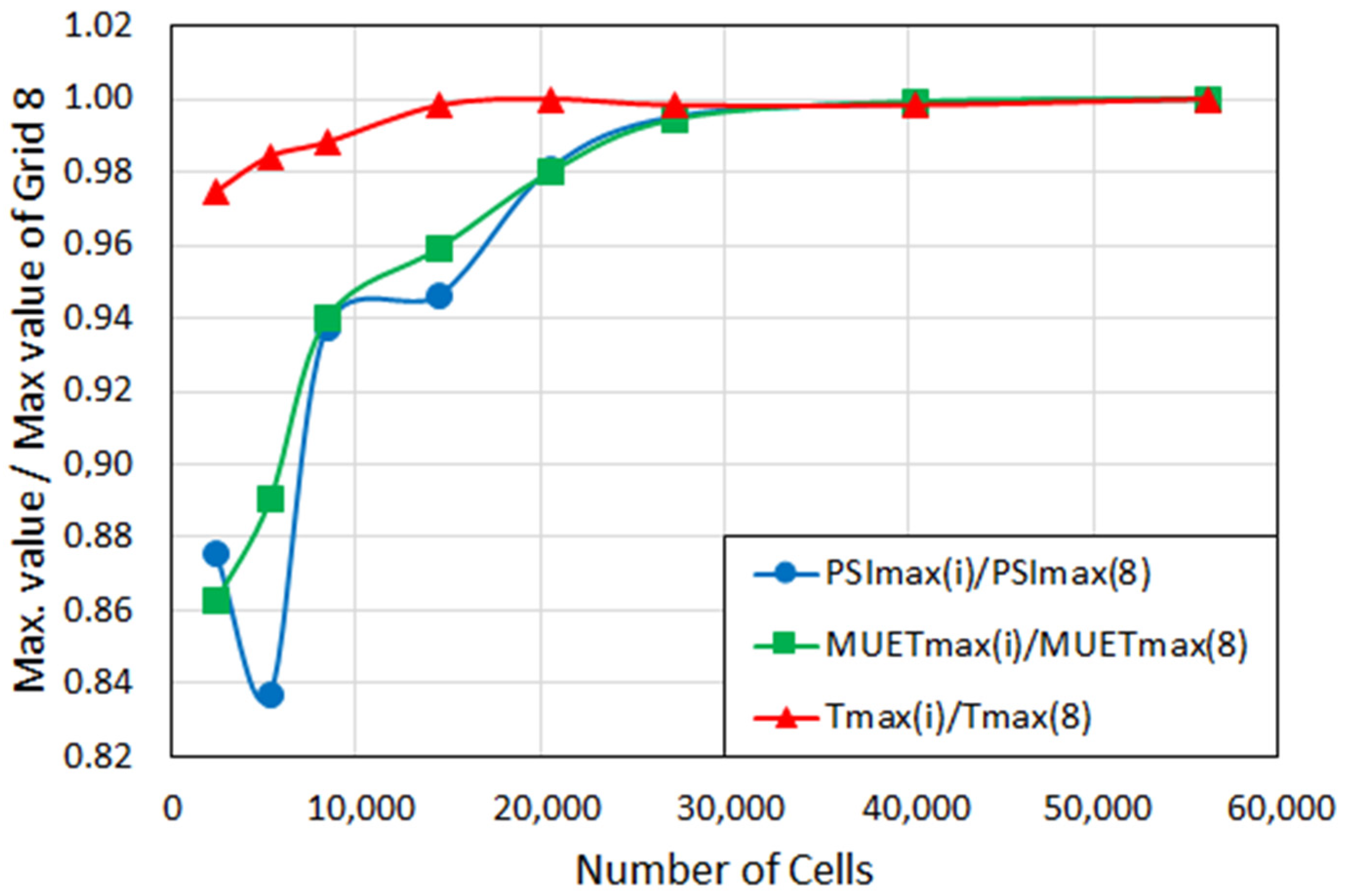
The geometry of the problem as well as the boundary conditions exhibit axial symmetries. This implies that the time-averaged solution, which is sought within the RANS framework, also needs to be axisymmetric. Consequently, the present problem is formulated as a two-dimensional-axisymmetric one, defining the solution domain to be as such. The total furnace length is considerably large compared to burner dimensions (Figure 1). Nevertheless, the measurements [61] indicate that the occurring flames are restricted to a comparably small zone downstream of the burner. Therefore, the whole combustor is not considered, and only a part up to 800 mm after the burner exit plane is defined as the solution domain in the present calculations. In a previous LES analysis of oxy-combustion with the same burner in the same furnace by Sadiki et al. [28], the considered domain size was 600 mm, which implies the sufficiency of the presently considered domain size. An additional issue in defining the solution domain in swirling flows is related to the outlet boundary. Particular attention is required in that respect since it can have a substantial effect on the upstream flow, specifically in the case of a sub-critical flow [63]. From a practical perspective, if a standard, classical “axial outflow” boundary is used at the outlet, convergence problems can easily emerge since the IRZ generated by vortex breakdown may extend to the outlet boundary and cause a reverse flow at the outlet. In order to reduce potential inaccuracies and computational difficulties in that respect, in our earlier investigations, we found [64] that it is suitable to replace the axial outlet with a radial outflow boundary without influencing the solution in the domain of interest. For the present case, additional calculations have been performed to ensure the adequacy of the present choice of the domain size and outlet boundary condition. The solution domain and the boundary types are depicted in Figure 2.
At all inlets, uniform profiles are defined for all of the variables that are transported convective-diffusively, which are in accordance with the fuel properties and the prevailing operating conditions, as shown in Table 4 and Table 5, above. For turbulence quantities, the inlet boundary conditions are obtained by assuming a turbulent intensity of 4% and a length scale as a function of the local hydraulic diameter. Additionally, an isotropic turbulence is presumed at the inlet boundaries. At the outlet boundary, the static gage pressure is defined to be zero together with the zero normal gradient conditions for all convective-diffusively transported variables. At wall boundaries, the no-slip condition holds for the momentum and turbulence model equations (complemented by the wall functions), as a zero normal gradient condition is applied for the species transport equations. There is some uncertainty in the thermal boundary conditions. The measured wall temperature data were not provided for air combustion in this burner. Inspired by the available experimental information on the oxy-combustion, a furnace wall temperature boundary condition of 900 °C is prescribed. A further uncertainty in the thermal boundary condition resides in the wall emissivity. In the absence of any experimental information, a wall emissivity of 0.7 is assumed. Inlet and outlet boundaries are assumed to behave as black surfaces for thermal radiation. Obviously, symmetry conditions apply on the symmetry axis.
For the particle phase, it is assumed that the particles are in dynamic and thermal equilibrium with the gas at the inlet. Particles are injected with a homogeneous distribution at the primary inlet. At the walls, the particles are assumed to be reflected by a normal and tangential restitution coefficient of 0.4, which approximately corresponds to experimental values found in the literature [65].

5. Grid Generation

In generating the grid, a block-structured strategy based on quadrilateral cells was adopted. A grid independence study was performed by employing the k-ε turbulence model under the assumption that this grid would provide satisfactory grid independence for the other turbulence models as well. Eight grids were used with the approx. number of cells: 2400 (Grid 1), 5300 (Grid 2), 8400 (Grid 3), 14,500 (Grid 4), 20,500 (Grid 5), 27,000 (Grid 6), 40,400 (Grid 7), and 56,000 (Grid 8). The predicted maximum values of the stream function (PSI), turbulent viscosity (MUET) and temperature (T) for different grids are displayed in Figure 3. In the figure, “normalized” values are displayed, where the maximum values obtained for a grid “i” (PSImax(i), MUETmax(i), Tmax(i)) are normalized by the maximum values obtained by the finest grid, i.e., Grid 8 (PSImax(8), MUETmax(8), Tmax(8)).
As it can be seen in Figure 3, the variations are very small beyond Grid 5, which has 20,500 cells. Thus, for the calculations, Grid 6 is used, which has 27,000 cells. In a previous study by Chen and Ghoneim [26] for the 100 kWth oxy-combustion flame in the same furnace, grid-independent results in 2D were obtained by a grid with about 20,000 cells. This can be seen as a further support for the adequacy of the present grid.

6. Predictions, Comparisons with Measurements

The prediction results are presented and compared with the measurements in this section. Averaged velocities and temperatures will always be presented for the turbulent flow in the form of a RANS formulation. By doing so, an explicit reference to averaging will not be made for the sake of simplicity. Please note that the temperature and species concentration measurements were not provided by Zabrodiec et al. [61] and that the measurements were only documented for the velocity field for the present flame. Thus, the validation of the models used here, i.e., comparison of the predictions with the measurements, will be primarily performed based on the velocity field.

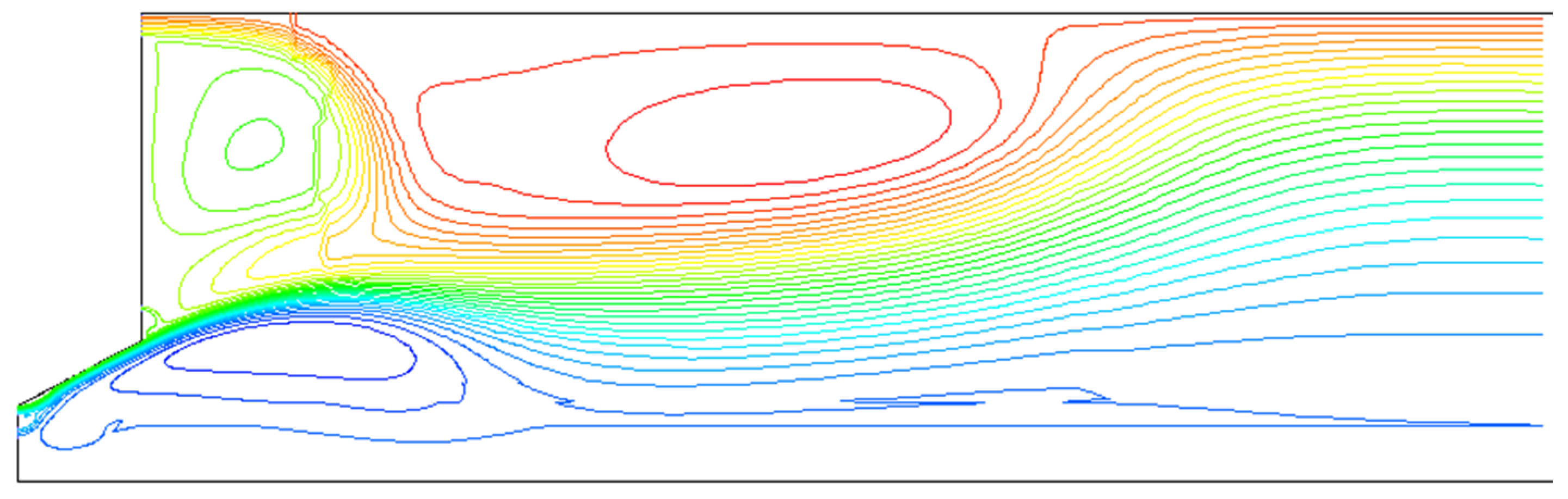
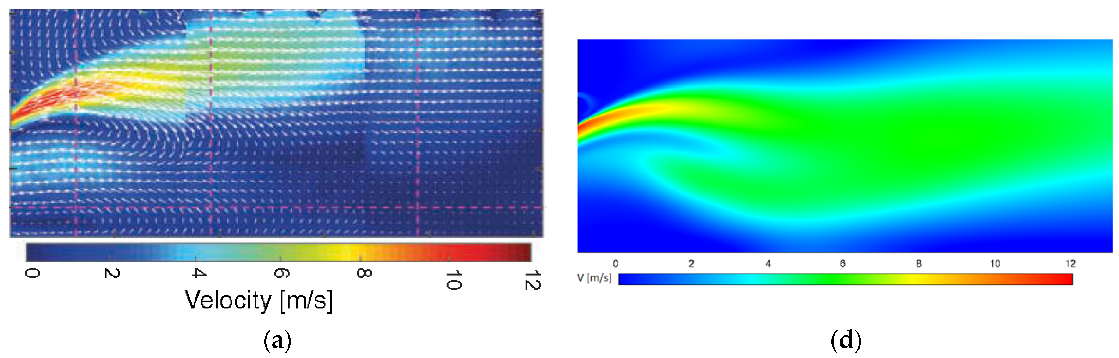
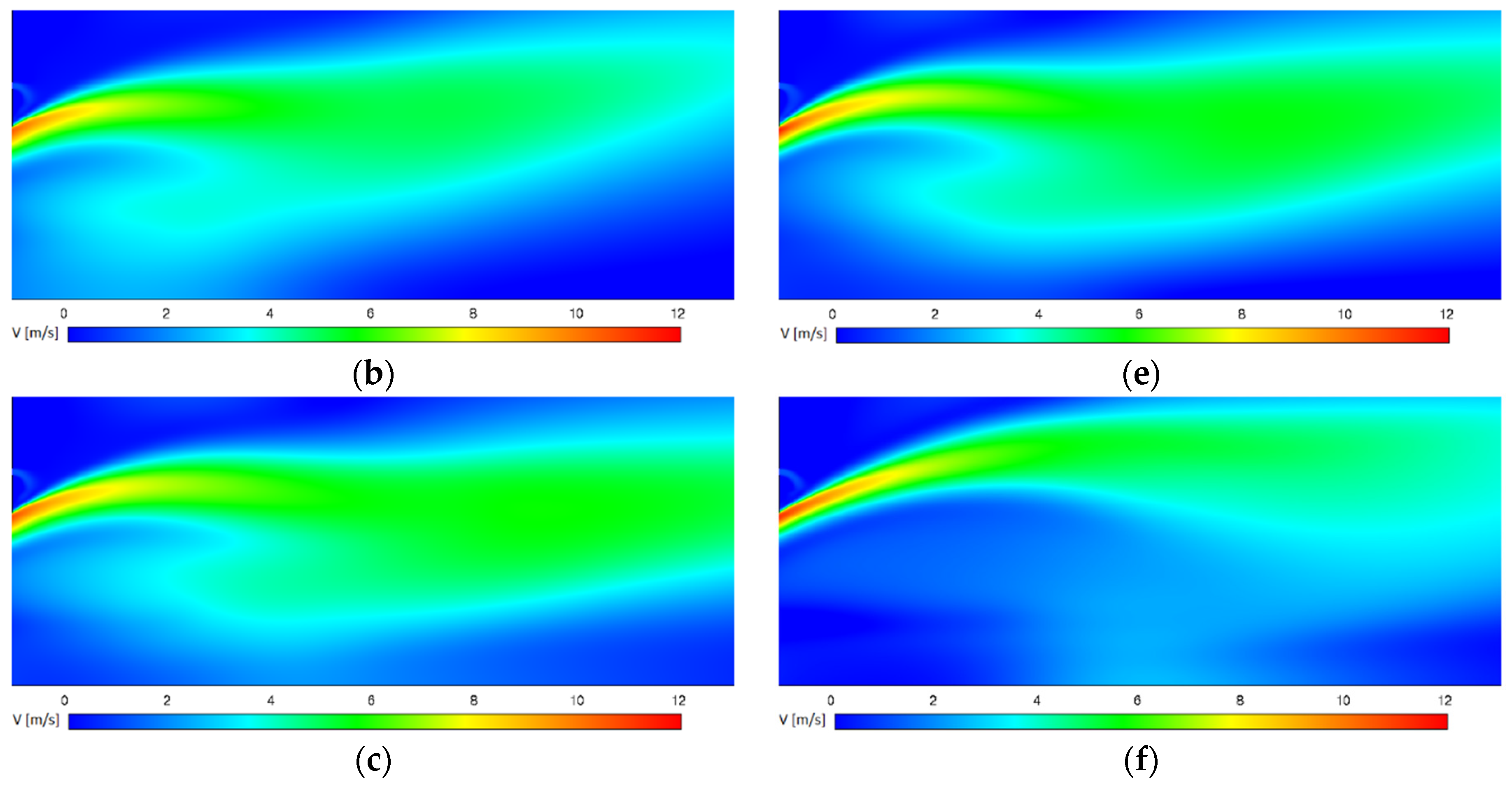
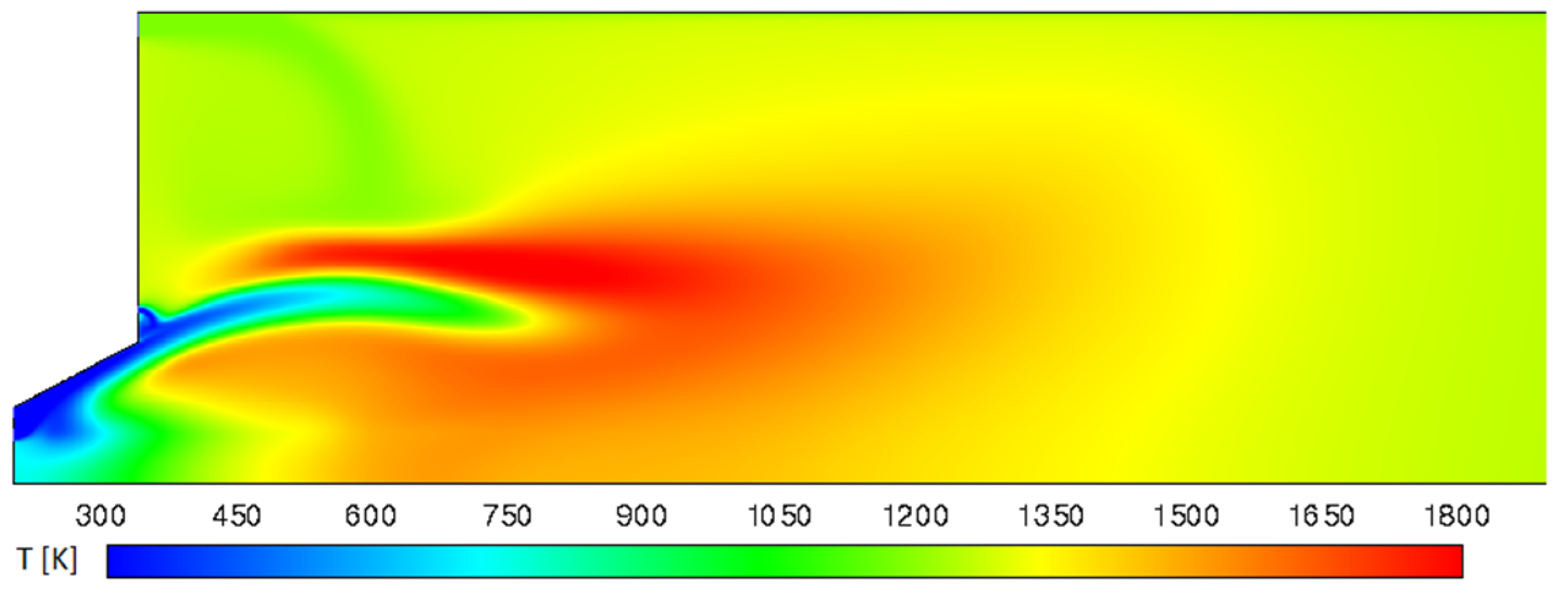
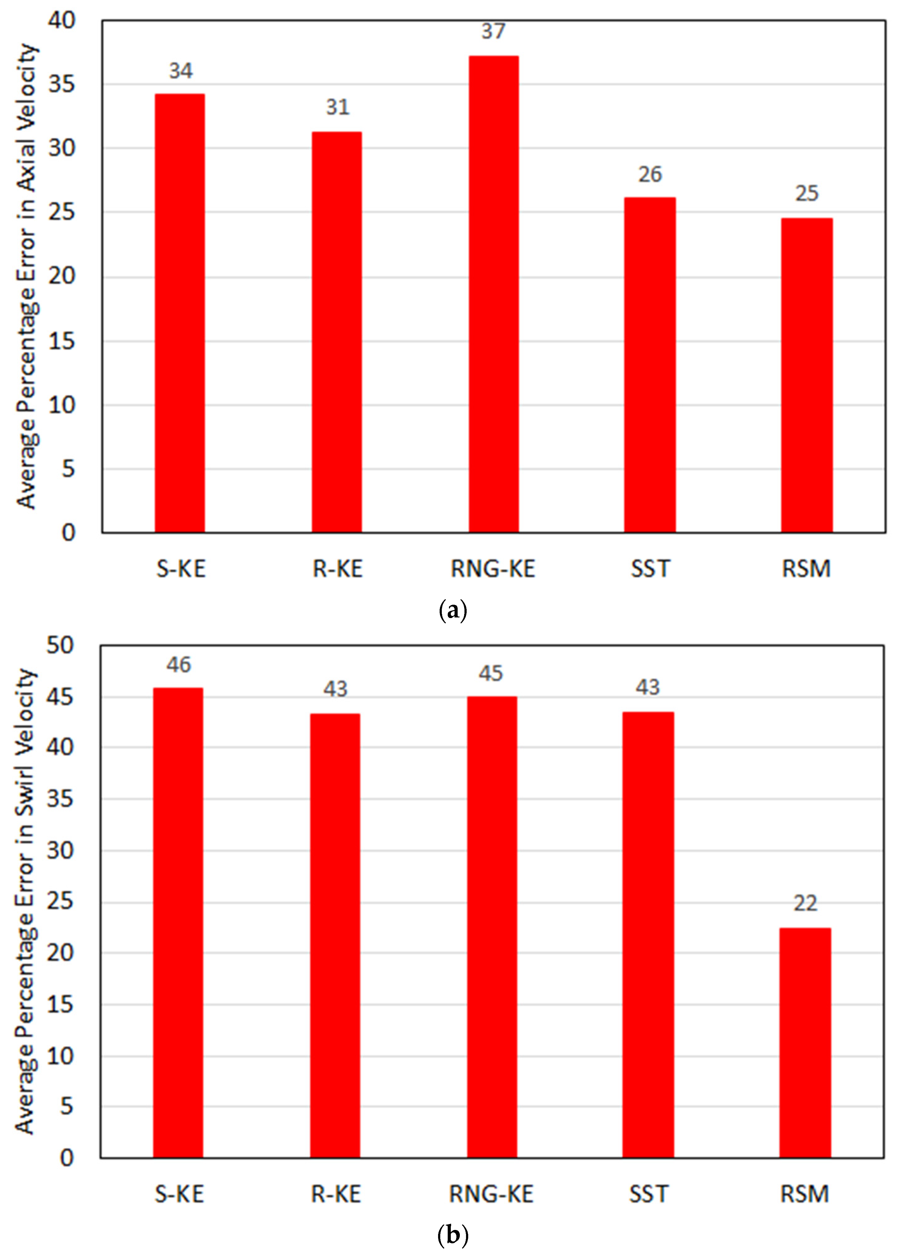
6.1. Field Distributions
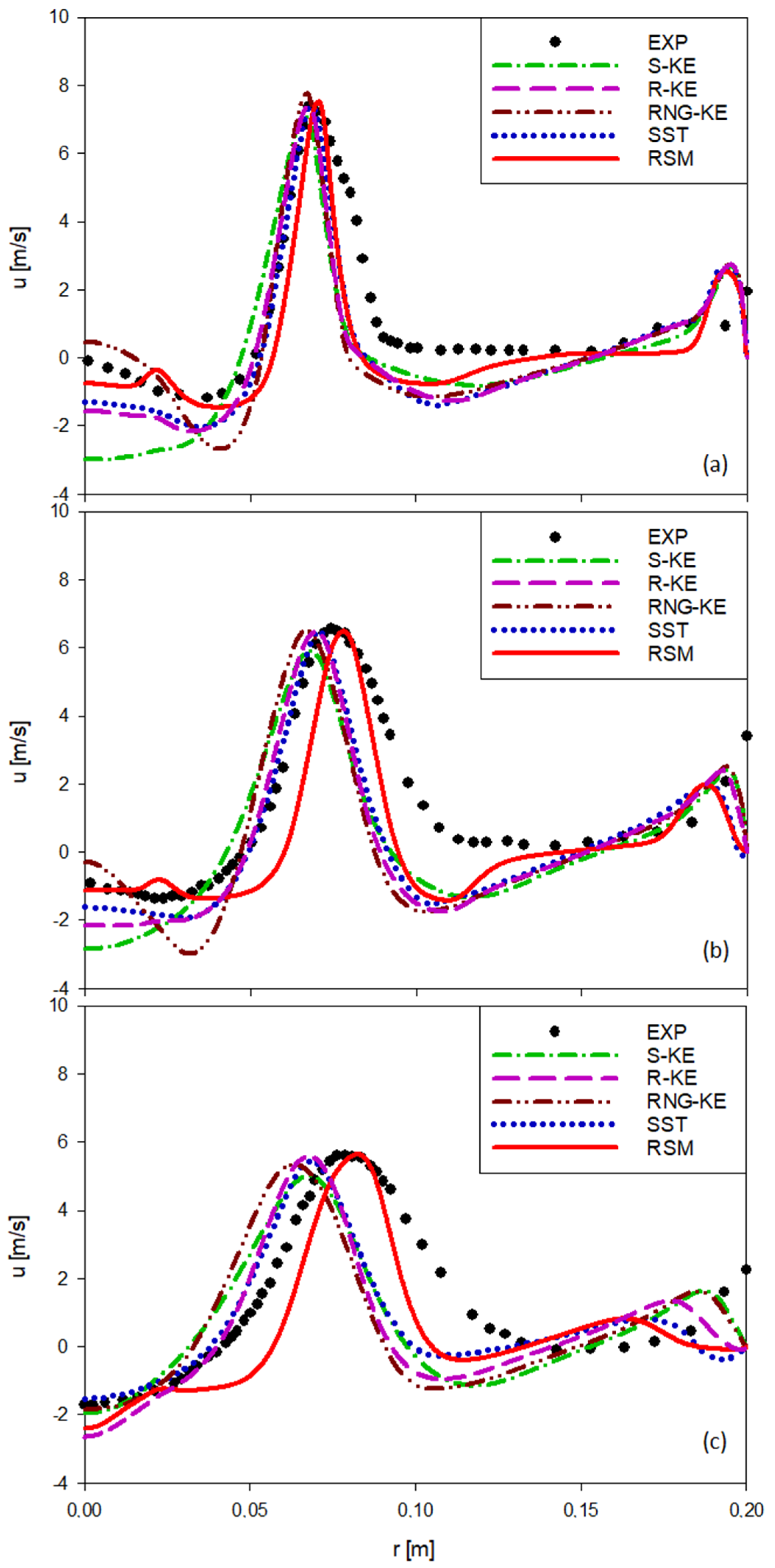
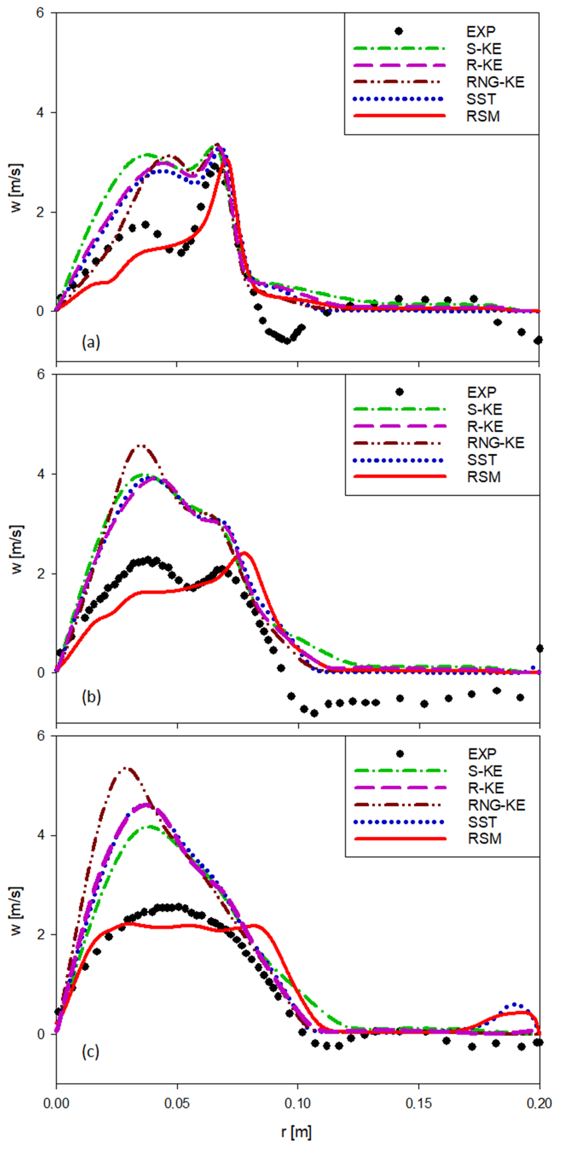
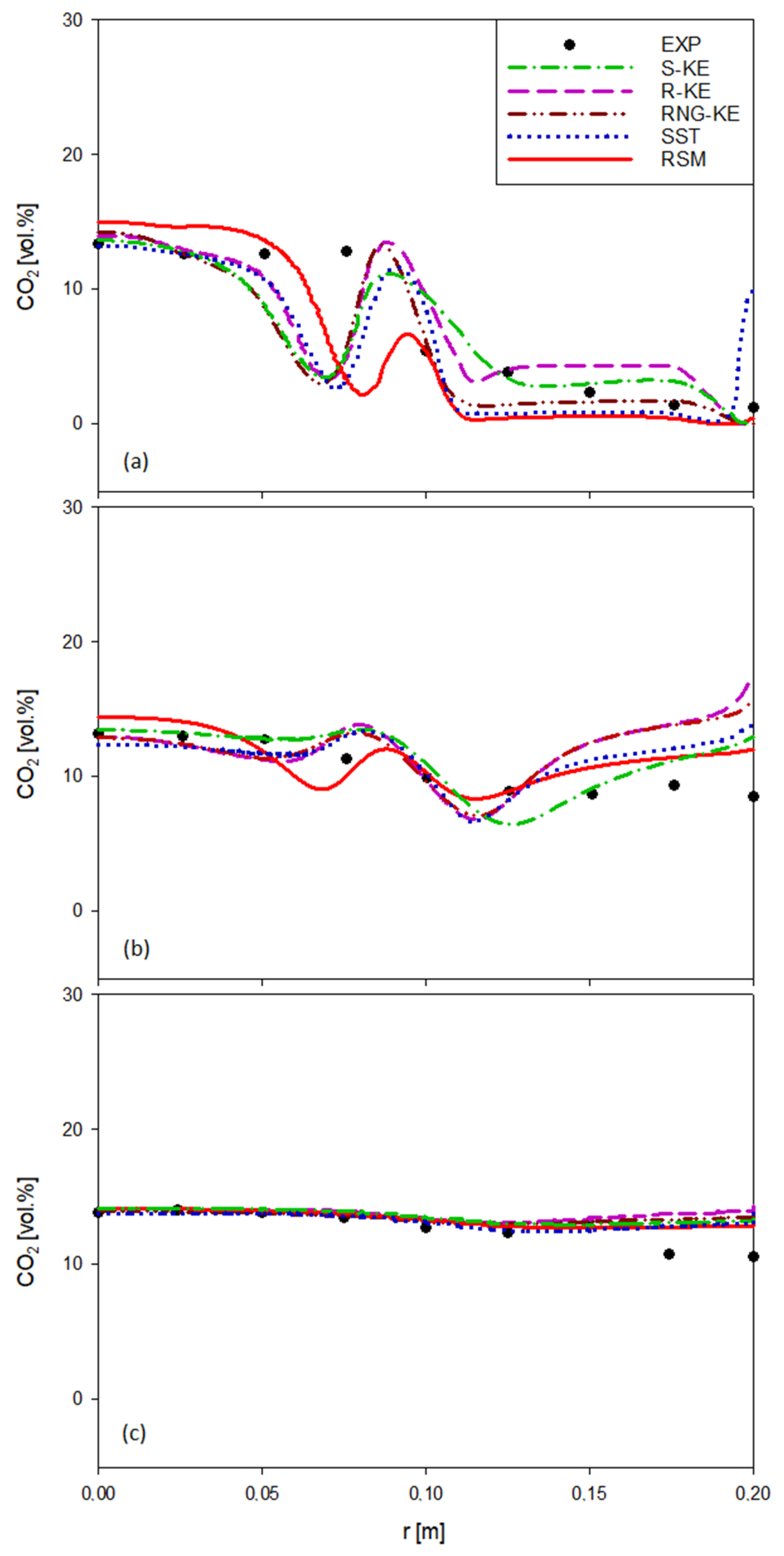
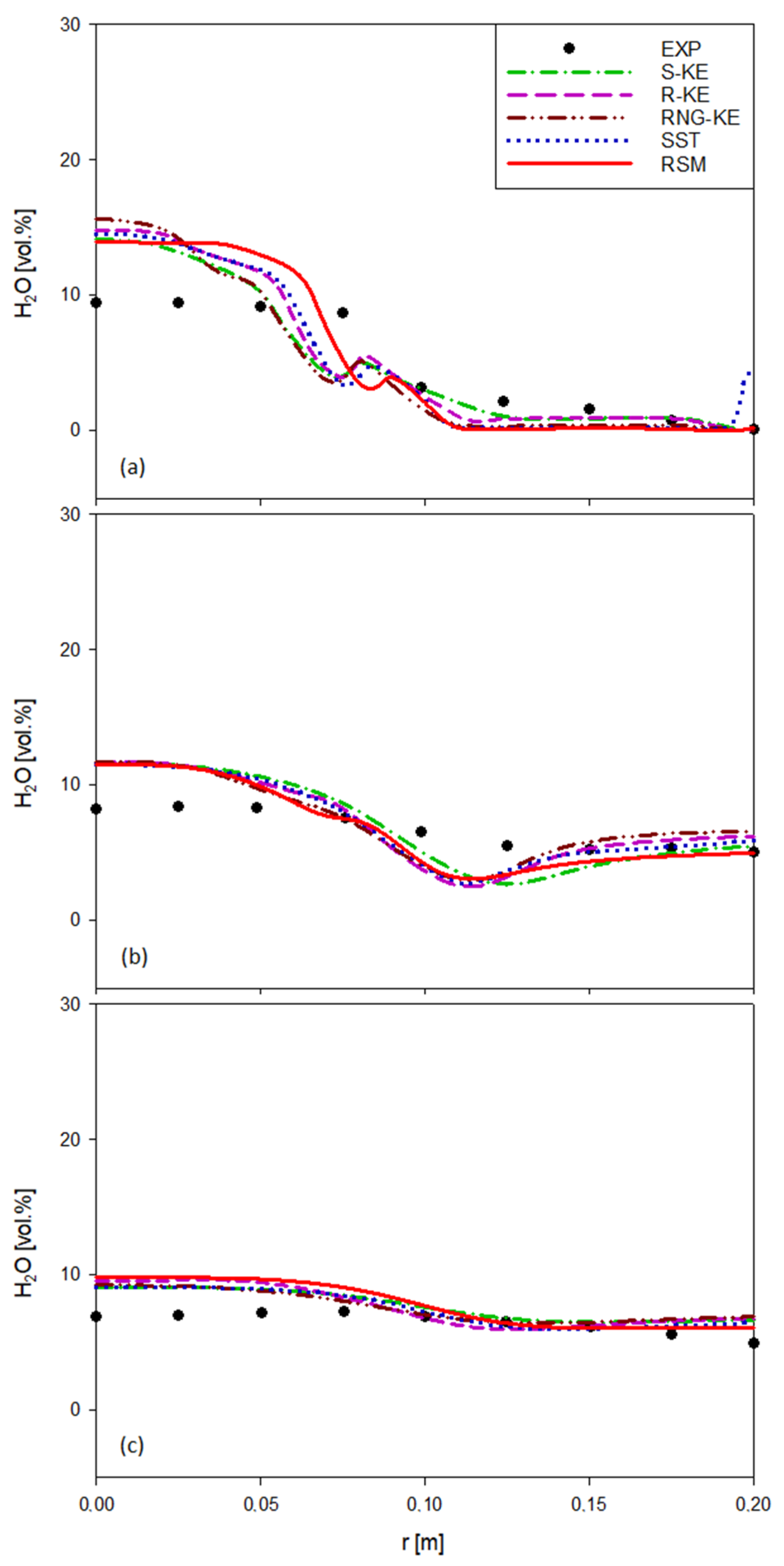
An overview of the general flow structure in the furnace can be gained from the streamlines. The predicted streamline patterns by different models are qualitatively similar. Thus, the general flow structure is discussed based on only one of the models. The predicted streamlines by the RSM are presented in Figure 4.
One can see that the general flow pattern is governed by three recirculation zones. The centrally located internal recirculation zone (IRZ) in the burner quarl and its downstream, which is typical for swirling flows with vortex breakdown, can be easily observed. In the outer region, two recirculation zones can be identified, which are created with the action of the staging air stream. The staging air is injected as a wall jet along the furnace jacket. It is interesting to observe how it separates from the wall with the action of the swirling free jet and mixes with it.
Measured [61] and predicted fields of the velocity magnitude in the burner nearfield, within the region 0 ≤ x ≤ 250 mm, and 0 ≤ r ≤ 100 mm are displayed in Figure 5, where the flow structure in the burner zone can be observed in more detail. One can see that the jet-like forward flow with high velocity leaving the outer wall of the conical burner quarl is directed diagonally with a radial component and is under the influence of the centrifugal force field due to swirl. The IRZ at the outlet of the burner quarl as well as a external recirculation zone with comparably low velocities can also be observed. With the increasing axial distance, one can see that the forward jet expands and takes a more axial direction in a manner that envelopes the internal recirculation zone.
This qualitative trend is observed in the experimental and all predicted fields displayed in Figure 5. The predicted maximum velocities by all of the models agree well with the measured value. However, the decay of the maximum velocity in the axial direction is slightly overpredicted similarly by all models. As far as the deflection of the jet towards the axial direction is concerned, all models except the RSM show an overprediction, i.e., an earlier deflection of the jet compared to the experiments. In this respect, the RSM results seem to agree better with the measurements. The RSM results show a better agreement with the experimental results for the contour of the outer edge of the jet. The radially inward spread of the jet is, however, underpredicted (Figure 5).
The temperature fields predicted by all of the models were qualitatively similar. Temperature distribution in the burner nearfield (for x < 600 mm) as predicted by the RSM is presented in Figure 6.
One can see that the cold mixture enveloped by the reaction zone (flame brush) leaves the outer edge of the conical burner quarl and extends into the furnace, resulting in a “tongue”-like shape. Under the influence of the centrifugal force field generated by the swirl, the direction of the flow has a radial component at the burner outlet, which takes a more axial orientation with increasing distance from the burner, as already discussed above. The forward flow of the cold mixture is surrounded by high-temperature regions. In the central part (IRZ), the temperatures are high because of the combustion reactions and recirculating hot gases. The outer high temperature zone is greatly affected by the staging air. The staging air introduced as a wall jet separates from the furnace wall at a distance of approximately 50–100 mm and mixes into the swirling jet, causing a local intensification of the combustion reactions in the mixing zone, as it supplies the necessary amount of additional air to achieve complete combustion.

6.2. Line Plots

The radial variations of the axial velocity (u) at three axial stations are presented in Figure 7, where the predictions obtained by different turbulence models are compared with the measured values [61].
Looking at the profiles of the axial velocity (Figure 7), an internal recirculation zone (IRZ) with negative velocities can be observed, with this internal recirculation zone extending between the centerline and the radial position at about r = 0.04–0.06 m, which is typical for swirl-stabilized flames. A weaker outer recirculation zone, with negative velocities approx. between 0.095 m and 0.12 m, can also be seen to be indicated by all profiles. Between both recirculation zones, the forward flow region with high axial velocities can be observed. In general, the radial extension of the forward flow region (Figure 7) is underpredicted by all models, which was also deduced in Figure 5. The peak velocity of the forward flow is the highest at the most upstream position (x/D = 0.5) and becomes gradually reduced in the downstream (Figure 7).
The peak axial velocities of the forward flow region are predicted very well by all turbulence models, where a slightly better performance of the RSM can be observed (Figure 7). The measured velocities in the central regions, i.e., within the IRZ, show an interesting trend for x/D = 0.5 and x/D = 1.0, where maximum negative recirculation velocity is not observed on the centerline (r = 0) but at an off-centerline position (r = 0.03–0.04 m). This behavior is qualitatively predicted by all turbulence models except the S-KE. At x/D = 0.5, the quantitatively best prediction is provided by the RSM. The RNG-KE results are also close to the measured values in the centerline but overestimate the negative recirculation velocities around r = 0.04 m. It is interesting to note that the R-KE and SST results are quite close to each other. At x/D = 1.0, the velocity values within the IRZ are predicted by the RSM very well. RNG-KE strongly overestimates the curvature of the velocity profile. The R-KE and SST results are again quite similar, and the SST results are slightly better than those of R-KE on the centerline as well as along the outer shear layer. As was the case for both x/D = 0.5 and x/D = 1.0, the S-KE does not perform as well as the other models in the central parts in the IRZ. However, outside of the IRZ and beyond r = 0.04 m, the performance of the S-KE is very similar to the other TV models (R-KE, RNG-KE, SST) and is even partially better for all three axial stations. At x/D = 1.0, although the RSM predicts the velocities in the central parts well, it overpredicts the radial extension of the IRZ, as the other turbulence models agree with the measurements in this respect better. On the other hand, in the outer shear layer, the RSM results are closer to those of the experiments compared to the other models. At x/D = 1.5, the position and magnitude of the peak velocity is predicted by the RSM very well and is clearly predicted better than the TV models. Among the TV models, a relatively better performance of the R-KE and SST can be observed. The R-KE and SST deliver similar results in the IRZ but show some deviation in the outer region, where the SST results are closer to the RSM ones.
The radial variations of the swirl velocity (w) at three axial stations are presented in Figure 8, where the predictions obtained by different turbulence models are compared to the measured values [61].
Generally, two distinct regions can be identified at all three axial stations.
The higher swirl velocities are observed in the central parts (r < 0.1 m) that exhibit remarkable radial variations, with a solid body-like vortex core confined to the central region (r < 0.02–0.03 m). The position of the vortex core (Figure 8) is seen to be practically coincident with that of the IRZ (Figure 7).
In the outer region (r > 0.1 m), quite low and almost homogeneous swirl velocities are observed. Here, all of the models show very close predictions to each other and a generally fair agreement to the measurements. A rather distinct difference to the measurements in this region (r > 0.1 m) can be observed at x/D = 1.0. At this axial position, negative swirl velocities were measured, and these could not be calculated by the models that could only predict low but positive swirl velocities. This rather unexpected trend with a negative swirl, which was observed in the measurements, was probably caused by three-dimensional effects, which were not possible to predict with the present two-dimensional-axisymmetric formulation. The following discussion on the swirl velocity profiles refers to the inner region (r < 0.1 m), where, in contrast to the outer region (r > 0.1 m), substantial differences between the curves are observed.
At x/D = 0.5, the experimental curve exhibits two distinct swirl velocity peaks. The outer peak, which is the stronger one, is well predicted by all of the models. The inner peak is predicted qualitatively by the TV models, which, however, overpredict the experimental value quantitatively. The inner peak is only weakly indicated by the RSM. However, the best overall quantitative agreement throughout is provided by the RSM.
At x/D = 1.0, the double peak structure of the experimental curve is retained, where both peaks have similar strength. The RSM results agree quite well with the measurements, with the outer peak being well-predicted. All of the TV models strongly overpredicted the measurements at x/D = 1.0.
At the third axial station, at x/D = 1.5, the double peak structure of the swirl velocity vanishes. The RSM agrees, again, very well with the measurements, both qualitatively and quantitatively, whereas the TV models strongly overpredict the experimental values.
For the TV models, one can see that their predictions are qualitatively very similar and quantitatively not very much different from each other at all three axial stations. One can again see that the R-KE and SST predictions are very similar to each other throughout. The RNG-KE prediction is slightly better than those at x/D = 0.5, but it becomes increasingly less accurate at further axial stations at x/D = 1.0 and 1.5. The S-KE shows the reverse trend, which demonstrates improving accuracy with axial distance.
To support an overall assessment, the percentage deviations of the predictions from the measurements were calculated as average values for the axial and swirl velocities. Based on the curves presented in Figure 7 and Figure 8, radially averaged values for the percentage deviation of the predictions from the experiments were calculated as χ = 100 × (1/R) ∫(|ϕEXP(r) − ϕPRED(r)|/ϕREF) dr) at each of the three axial stations, where ϕ denotes either u or w and where the reference value (ϕREF) is taken as the half of the difference between the maximum and minimum experimental values at the considered axial station (ϕREF = (ϕEXP,max − ϕEXP,min)/2). The percentage deviations obtained at each of the three axial stations were then arithmetically averaged to obtain an overall averaged value for each turbulence model. The overall percentage deviations from the experiments for the considered turbulence models, which were calculated in this manner for the axial and swirl velocity components, are presented in Figure 9.
One can also see that in this type of “overall” comparison, RSM performs better than the TV models, which is clearer for the swirl velocity (Figure 9b). As far as the TV models are concerned, the SST is close to RSM and thus performs better than the others for the axial velocity (Figure 9a). As far as the swirl velocity is concerned, no significant difference between the TV models can be observed, and the RSM accuracy is nearly twice as better compared to the TV models (Figure 9b).
Measured values of the CO2 and H2O volume fractions for the present flame were provided in a recent publication by Nicolai et al. [30]. The radial variations of CO2 volume fractions at three axial stations are presented in Figure 10, where the predictions obtained by different turbulence models are compared to the measured values [30].
The measured CO2 profile at x/D = 1.0 indicates higher values in the central part (r < 0.1 m) of the furnace compared to in the outer region. This is qualitatively predicted rather well by all models, with a quite good quantitative accuracy for the values near the centerline and the wall, with the exception of the peak predicted by SST next to the wall. The transition from higher to lower values occurs monotonically in the measurements, whereas a wavy transition is predicted by the models. The latter is observed to be weaker for the RSM compared to the other models. At x/D = 3.0, the measured CO2 distribution is more homogeneous, which is also predicted fairly well by the models, which still exhibit a wavy structure at around r ≈ 0.1 m, but weaker. At x/D = 6.0 D, the measured CO2 distribution is very uniform, which is predicted quite well by all of the models, with the exception of a slight overprediction near the wall. Additionally, for x/D = 3.0 and x/D = 6.0, the RSM can be considered to show a slightly better overall performance compared to the other turbulence models (Figure 10).
Predicted radial H2O volume fractions profiles by different turbulence models are compared with the measurements [30] at the three axial stations in Figure 11.
The H2O profiles (Figure 11) show a similar qualitative trend to the CO2 profiles (Figure 10), exhibiting higher values in the central parts compared to the near wall region, with an increasing homogenization downstream. Additionally, for H2O, the models predict a wavy transition between the central and outer parts, around r = 0.1 m at x/D = 1.0 (Figure 11a). This is, however, less pronounced compared to CO2 (Figure 10a), leading to a better qualitative agreement with the measurements, which show a monotonic variation. On the other hand, the quantitative prediction of the values in the central region (r < 0.1 m), where an overprediction is observed, is not as good as that of CO2. The overprediction of the central values continues but also gradually diminishes further downstream at x/D = 3.0, x/D = 6.0 (Figure 11b,c). At x/D = 6.0, a rather homogeneous H2O distribution is predicted by all models, similar to what was seen during the experiments, but still has some overprediction in the central parts (Figure 11c). As far as the relative performance of the models based on the H2O profiles is concerned, a very clear distinction cannot be easily made, as a rather similar overall performance is observed. Based on the profiles at x/D = 1.0, the RSM may be considered to perform better since the “plateau”-type profile shape of the measurements (with nearly constant values between the centerline and r ≈ 0.08 m) is qualitatively better predicted by the RSM (Figure 11a).

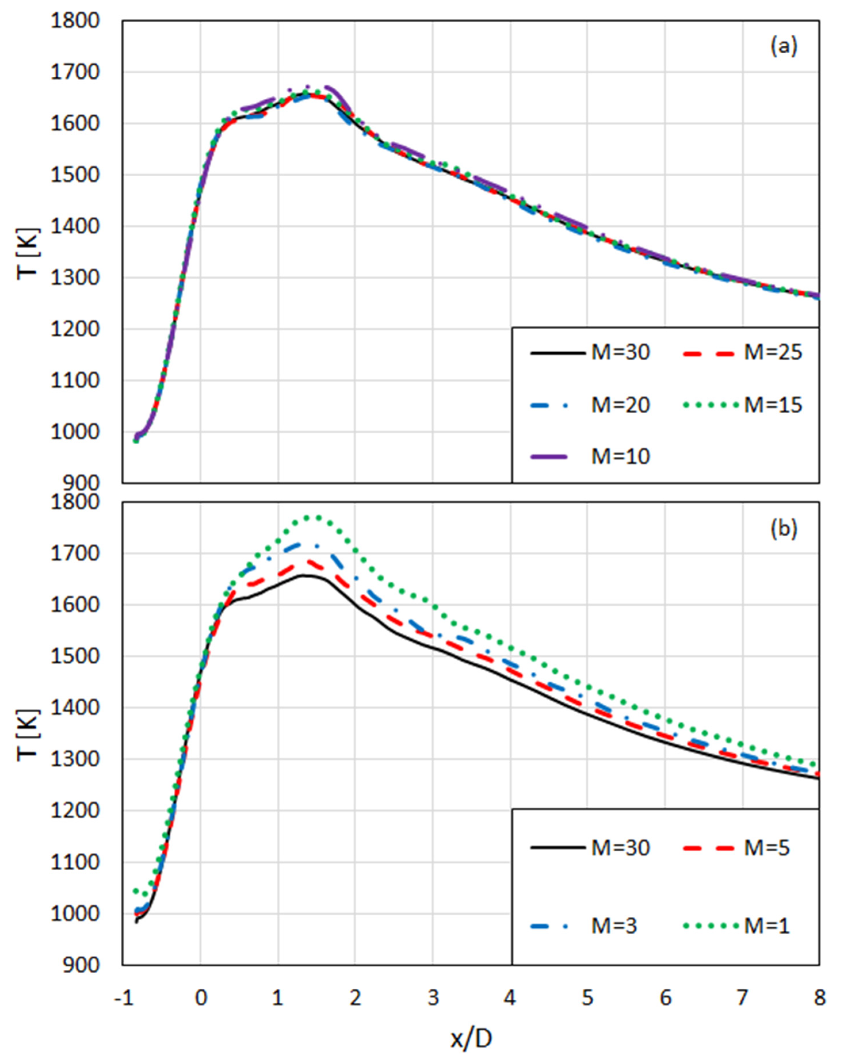
7. Investigations on the Resolution of the Particle Phase

7.1. Turbulent Particle Dispersion

As outlined above, the turbulent particle dispersion (TPD) is modelled by the discrete random walk model. Due to the randomness, a sufficiently large number of random trajectories (trials) need to be calculated to obtain representative mean values. The number of trials (M) has a direct influence on the computational costs. Thus, it is of interest to find an optimally low number that is still high enough to provide sufficient accuracy. In the present section, a study is performed using different trial values to investigate their effect on the results. Within this context, a comparison with the measurements is not necessarily relevant. It is more about the evolution of the numerical solution in itself, with varying M (similar to a grid independence study). Therefore, comparisons with measurements are not performed in this section. The study is performed based on the S-KE (which is due to pragmatic reasons since it exhibited the best convergence properties), assuming that the outcome of the study with respect to the effect of M would analogously apply to the other turbulence models. In all of these calculations, the particle size distribution (SD) is the same, i.e., the same as the one with N = 18 used in the validation studies presented above (Table 6).
The considered number of trials (M) is listed in Table 7. Note that M = 20 was used in the model validation studies presented above.
The differences between the solutions can be demonstrated in different forms based on different variables. For clarity, the variation of the solution with varying M is discussed based on the temperature variation along the furnace axis. The temperature curves for all eight M values are presented in Figure 12. For clarity, the curves are presented in two sub-figures.
One can see that the results for M = 30, 25, 20, 15 are nearly identical, and M = 10 only shows a minimal difference to them (Figure 12a). This confirms that the used value M = 20 in the validation was certainly high enough. Larger differences to M = 30 can be seen for M = 1,3,5, as shown in Figure 12b. The difference to the M = 30 curve is still quite small for M = 5. More substantial differences are observed for M = 3 and M = 1.
For a more quantitative overview, the results are compared in average percentage deviations to the most accurate solution with M = 30. Based on the curves presented in Figure 12, the average percentage deviations for different M are defined as χM = 100 × (1/L) ∫(|T30(x) − TM(x)|/T30(x)) dx), where the considered length (L) is taken to be 6D only, excluding the effect of the further downstream part (x > 6D). The average resulting percentage deviations are displayed in Figure 13.
As already observed in Figure 12, the deviations of the M = 25, 20, 15, 10 results from those of N = 30 are quite insignificant, and after a gradual increase for M = 5, larger differences are observed for M = 3,1, which are still rather small. Based on the above comparison (Figure 12 and Figure 13), one can conclude that M = 5 may be considered to be a quite optimal choice, as it provides quite good accuracy without being too high.

7.2. Resolution of the Particle Size Distribution

The measured particle size distribution (SD) [62] was provided by means of a cumulative distribution function based on 18 distinct sieve mesh sizes. In the above calculations, an SD is applied (Table 6), which is directly based on the experimental distribution, using 18 particle size classes (SC). As this is based on the experimental distribution and because the number of size classes (N = 18) is equal to the resolution of the data, one can assume that in this respect, the solution can be taken as a reference.
In CFD applications in general, the measured size distributions are not always directly applied. Instead, the distribution is approximated by a continuous function that then delivers the basis for a subsequent discrete distribution with the required resolution. In the first sub-section that follows, the aspects related to the approximation of the discrete SD by a continuous function are discussed. This is followed by a sub-section on the effect of the resolution in discretizing of the continuous distribution function.

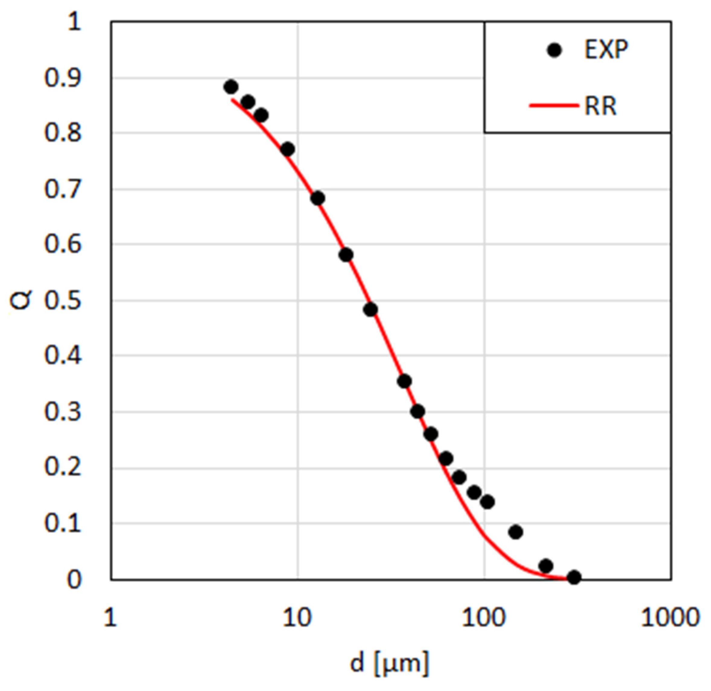
7.2.1. Representation by the Rosin-Rammler Distribution Function

A quite commonly applied analytical function to represent the SD in pulverized fuel combustion is the Rosin–Rammler distribution function (RR) [66]. Here, the mass fraction of particles (Q) with a diameter larger than “d” is expressed by the following equation:
Q = exp [ ( d d 0.632 ) n ]
where d0.632 (which corresponds to a diameter, for which the 63.2% of the total mass is of smaller diameter) and n (spread parameter) are constants that can be adjusted to fit the curve to the experimental distribution. Based on the measured distribution, the parameter d0.632 can be obtained. The spread parameter, n, can then subsequently be determined by curve fitting, minimizing the difference to the measured values.
For the presently given measured SD, the following values are obtained for the parameters of the RR: d0.632 = 36.15 μm, n = 0.91. The experimental distribution and its RR approximation are compared in Figure 14.
One can see that the agreement with the measured distribution and RR is fairly good. However, there are also deviations, as the measured distribution does not perfectly follow the assumed exponential pattern. The larger deviations are quite local and occur around d = 100–200 μm. As these diameters represent rather small mass fractions, their effect on the overall results may be expected to not be too large.
Having defined the RR, this needs to be discretized by a number of SC, which are distributed according to some rule in the diameter space. For the latter, one of the two procedures is normally applied in commercial software: The SC diameters are obtained by an equidistant division of the diameter range based (1) either on a linear diameter scale (LIN-RR) (2) or on a logarithmic diameter scale (LOG-RR). On the linear scale, the LIN-RR results in an equidistant distribution, whereas the LOG-RR results in a finer resolution towards the smaller diameters. Keeping the minimum and maximum diameters constant, the resulting RR (d0.632 = 36.15 μm, n = 0.91) is discretized by 18 SC, both linearly (LIN-RR) and logarithmically (LOG-RR), in the diameter space, and the resulting diameters of the 18 SC are compared with those of experiment (EXP) in Figure 15.
One can see that the LOG-RR represents the experimental resolution much more closely than the LIN-RR (Figure 15). For smaller diameters, the LOG-RR diameters are slightly smaller than the experimental ones, and for large diameters, the LOG-RR diameters are moderately larger than the experimental values. In LIN-RR, the diameters are distributed in such a way that considerably larger values than the experimental ones result for each size class (Figure 15).
For investigating the effect of using different types of RR discretizations, calculations were performed using the LOG-RR and LIN-RR distributions. Please note that the same RR and the same number of SC (N = 18) and the same number of trials (M = 20) were used, where only the distribution of the diameters of the SC in the diameter space was different. The S-KE was used as turbulence model, assuming that the result would be representative of the other turbulence models as well. The temperature variations along the furnace axis predicted by LOG-RR and LIN-RR are compared to that obtained by the experimental size distribution (Table 6) in Figure 16.
One can see that the LOG-RR does not agree perfectly well with the EXP curve although the same number of size classes (N = 18) was used, and the distribution of the diameters was not too different, showing that apparently small differences in the distribution can play a role. Obviously, the LIN–RR curve shows a larger deviation from the EXP curve since the differences in the diameters of the size classes deviated from the experimental values more strongly (Figure 15). This comparison shows that care is needed to approximate experimental distributions using the RR.

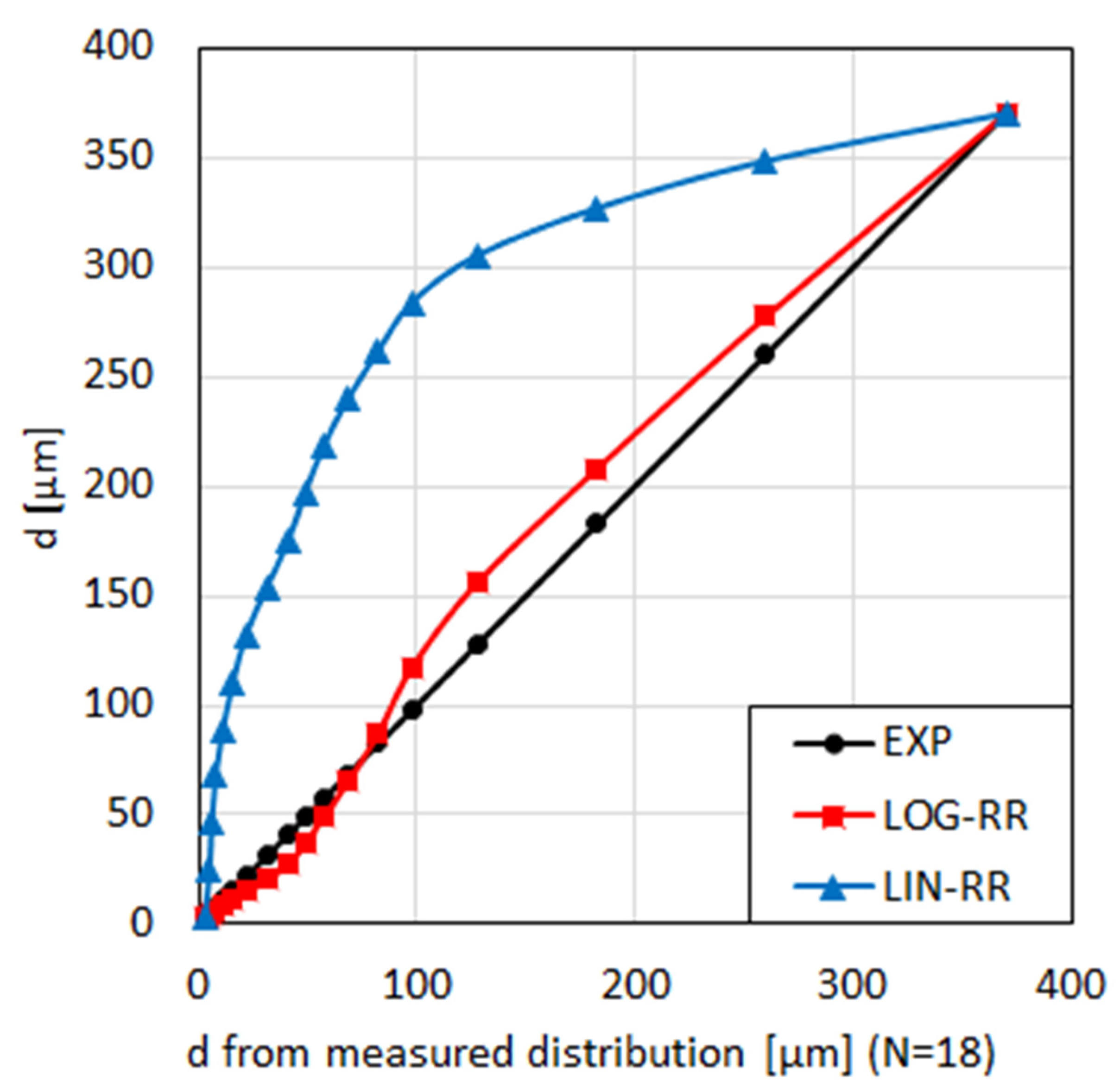
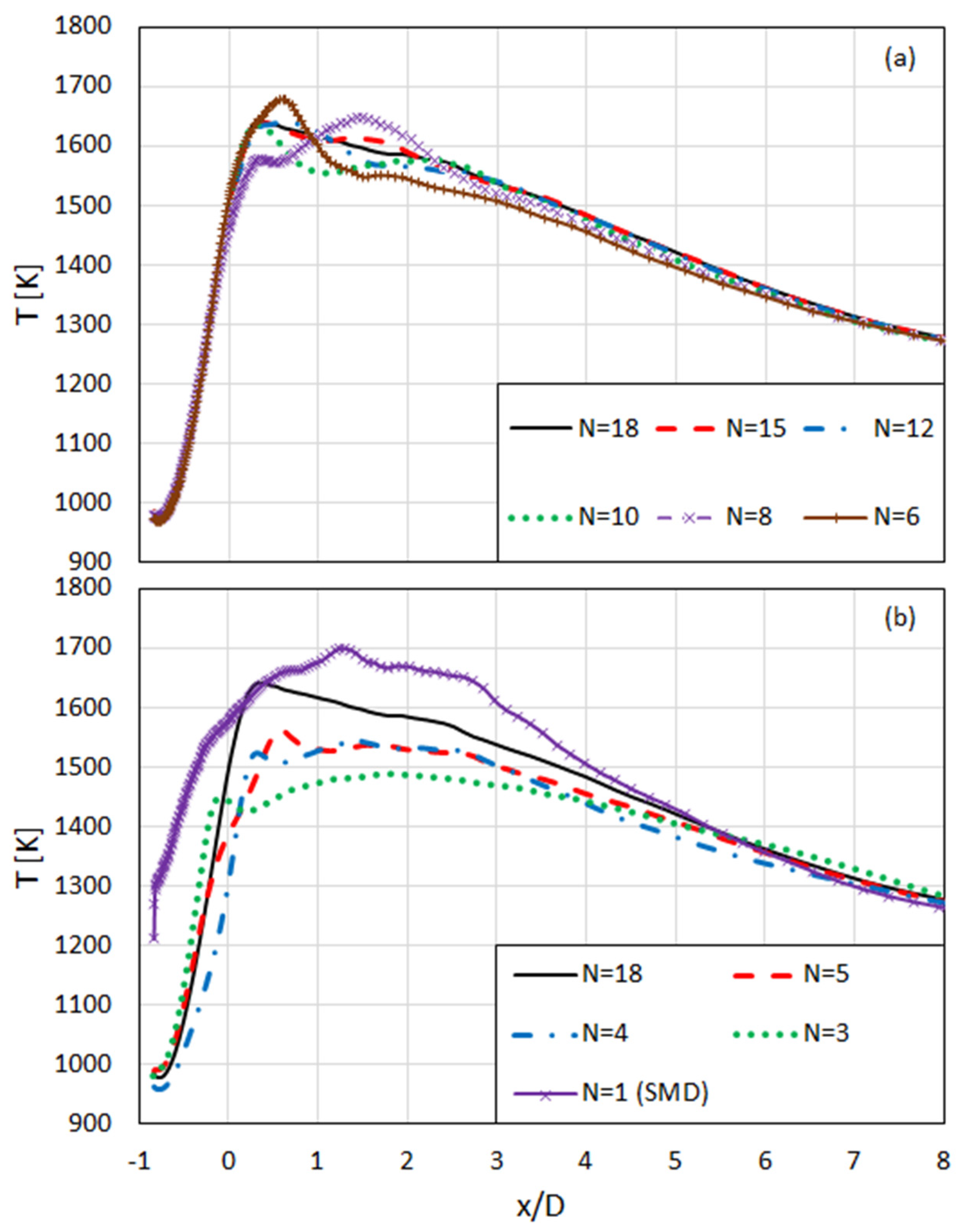
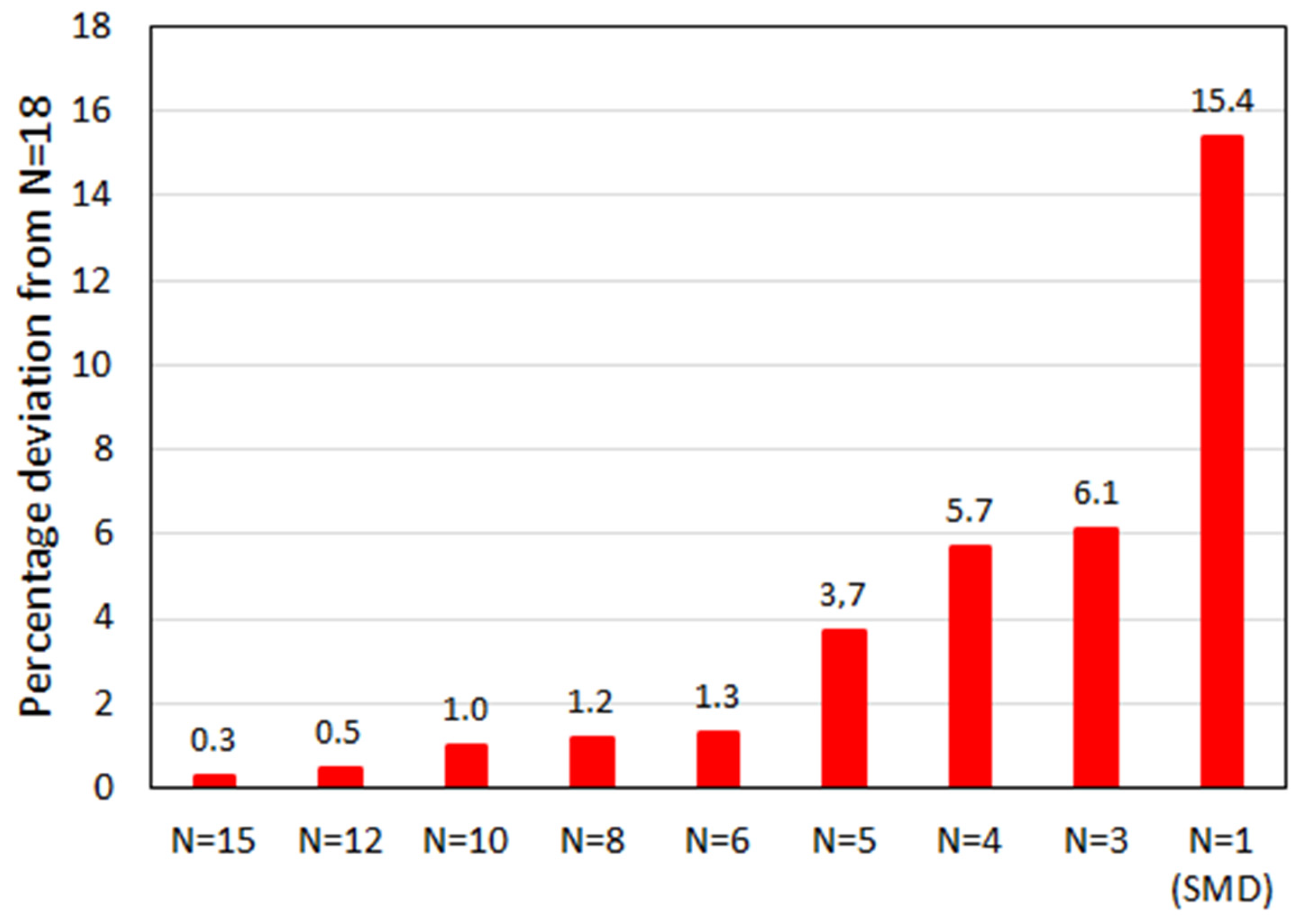
7.2.2. Resolution of the Particle Size Distribution

Having defined the RR and the rule for its discretization, the resolution of the discretization, i.e., the number of SC (N), needs to be defined. It is also important to find an optimal value for N here since it has a direct influence on the computational costs. This section deals with this question, investigating the effect of N on the solution. Here, the resolution of the experimental data, i.e., N = 18 taken as the highest resolution, and the effect of using a smaller N is investigated on the basis of LOG-RR distribution. The study is performed using the S-KE as a turbulence model and assuming that the outcome would analogously apply to the other turbulence models. In all of the calculations, the number of trials used to model the turbulent particle dispersion is the same, with M = 20.
The 10 total N values that were investigated are listed in Table 8. For all N, with the exception of N = 1, the diameters of the size classes are obtained from LOG-RR distribution. For N = 1, the diameter of the single size class is taken to be equal to the Sauter mean diameter (SMD) [66].
The differences between the solutions for varying N are demonstrated based on the temperature variation along the furnace axis in Figure 17. For clarity, the curves are presented in two sub-figures.
One can see that the results are sensitive to the number of size classes and that the deviations from the N = 18 solution increase with decreasing N. One can see that the N = 15 and N = 12 results are very close to those of N = 18 and moderate deviations are observed from the latter for N = 10,8 and 6 (Figure 17a). One can also observe that significant deviations to the N = 18 solution start to occur with decreasing N beyond N < 6 (Figure 17b).
For a more quantitative overview, the results are compared in average percentage deviations to the solution with highest resolution with N = 18. Based on the curves presented in Figure 17, the average percentage deviations for different N are defined as χN = 100 × (1/L) ∫(|T18(x) − TN(x)|/T18(x)) dx), where the considered length (L) is taken to be 6D only and only excludes the effect of the further downstream part (x > 6D). The average resulting percentage deviations are displayed in Figure 18.
Based on the above results (Figure 17 and Figure 18), N ≥ 12 can be considered to deliver a quite high accuracy. The results for N values between 10 and 6 (10 ≥ N ≥ 6) can still be considered to be moderately close to those of N = 18. The deviation of the results from those of N = 18 starts to grow more rapidly for N ≤ 5 (Figure 18).

8. Conclusions

A swirling pulverized coal flame was computationally investigated. The two-phase flow was described by a Eulerian–Lagrangian formulation. Turbulence was modelled by different RANS models, including the TV-based S-KE, R-KE, RNG-KE, and SST models as well as the RSM. The predicted velocity fields were compared with the measurements from Zabrodiec et al. [61]. The predictions were observed to deviate from the measurements within the range 20–40% in terms of the overall average values. It was observed that the velocity fields predicted by the RSM are closer to the measured values compared to the TV models, especially for the swirl velocity, where the overall accuracy of the RSM accuracy is twice as good as that from the TV models. Beyond the overall averages, the RSM was observed to mimic the local variations of the experimental curves better than the TV models did. Among the TV models, the overall performance of the SST model was better than that of the other TV models and was closer to the RSM results, especially for the axial velocity. It is interesting to see that the performance of the RNG-KE turned out to not be very well in the present application, falling behind both SST and R-KE, although it was generally expected to be accurate for swirling flows. The main deficiency of the S-KE compared to the other TV models was observed to be its inability to qualitatively predict the axial velocity profile in the IRZ in the burner nearfield. In further features of the velocity field, its performance was generally comparable to the other TV models.
It was demonstrated that inaccuracies can occur when approximating a size distribution using a Rosin–Rammler distribution function, and the importance of the particular choice in its discretization in defining the size class diameters was discussed.
The number of trials in the random walk model of TPD (M) and the number of size classes (N) for discretizing the SD had a direct influence on the computational costs. The present investigation on M showed that even 5 (M = 5) trials are sufficient for the highly accurate representation of the TPD and can lead to results with a less than 1% mean deviation from those of with M = 30. The N investigation indicated that more than 10 size classes (N ≥ 10) are needed for high accuracy and where N = 12 leads to results with a smaller than 1% deviation from those of N = 18 (the experimental resolution). Thus, M = 5 and N = 12 can be considered to be optimal choices for the discrete representation of the particle phase.
Although these numbers may not yet be claimed to have sufficient universality, they may serve as guidance, at least for SD with similar characteristics.
Although the present results on M and N were obtained in a 2D-axisymmetric analysis, they are applicable and even more needed in a three-dimensional analysis, where the optimal choice of these parameters is much more critical.

Author Contributions

Conceptualization, A.C.B.; methodology, A.C.B.; software, A.C.B.; validation, A.C.B. and C.D.C.; formal analysis, A.C.B. and C.D.C.; investigation, A.C.B. and C.D.C.; resources, A.C.B.; data curation, A.C.B. and C.D.C.; writing-original draft preparation, A.C.B.; writing-review and editing, A.C.B., C.D.C. and Y.E.B.; visualization, A.C.B. and C.D.C.; supervision, A.C.B. and Y.E.B.; project administration, A.C.B. and Y.E.B.; funding acquisition, A.C.B. All authors have read and agreed to the published version of the manuscript.

Funding

This research was partially funded by the Heinrich Hertz Foundation [B 42 Nr. 5/20].

Institutional Review Board Statement

Not applicable.

Informed Consent Statement

Not applicable.

Data Availability Statement

Presented data may be made available upon request from authors.

Acknowledgments

Financial support by the Heinrich Hertz Foundation is gratefully acknowledged.

Conflicts of Interest

The authors declare no conflict of interest.

Nomenclature

APParticle surface area (m2)
CDDrag coefficient (-)
cPParticle specific heat capacity (J kg−1 K−1)
DOuter diameter of secondary air nozzle (m)
dParticle diameter (m, μm)
dSSieve mesh size (μm)
d0.632Characteristic particle size in RR distribution
GIncident radiation (W m2)
hSpecific standardized enthalpy (J kg−1)
J φ , i t Reynolds flux vector of variable φ (corresponding units)
kTurbulence kinetic energy (m2 s−2)
kiRate coefficient of reaction i (s−1)
LFurnace length (m)
MNumber of particle random walks (trials)
mPParticle mass (kg)
NNumber of particle size classes
NuNusselt number (-)
nParameter in RR
PrPrandtl number (-)
pPressure (Pa)
QRosin–Rammler distribution function (-)
RFurnace radius (m)
RePParticle relative Reynolds number (-)
RetReynolds number of turbulence (-)
rRadial coordinate (m)
ScSchmidt number (-)
TStatic gas temperature (K)
TPParticle temperature (K)
tTime (s)
trParticle relaxation time (s)
uAxial velocity (m s−1)
uiGas velocity vector (m s−1)
ui,PParticle velocity vector (m s−1)
VVelocity magnitude (m s−1)
wSwirl velocity (m s−1)
xAxial coordinate (m)
xiCartesian coordinates (m)
YiMass fraction of species i
Greek Symbols
δijKronecker delta
ΔmMass fraction in a particle size class
εDissipation rate of k (m2 s−3)
εPParticle emissivity (-)
λThermal conductivity (W m−1 K−1)
μViscosity (Pa s)
μtTurbulent viscosity (Pa s)
ρGas density (kg m−3)
ρPParticle density (kg m−3)
τ i j t Reynolds stress tensor (Pa)
σStefan–Bolzmann constant 5.6704·10−8 (W m2 K4)
χPercentage deviation (-)
ωSpecific dissipation rate of k (s−1)
Sub- and Superscripts
PParticle
tTurbulent
VWVolatile matter
WWater
0Initial value
Abbreviations
ARAs Received
CFDComputational Fluid Dynamics
DAFDry Ash Free
HHVHigher Heating Value
IRZInternal Recirculation Zone
LESLarge Eddy Simulation
LHVLower Heating Value
R-KERealizable k-ε Model
RANSReynolds Averaged Numerical Simulation
RNGRenormalization Group Theory
RNG-KERNG k-ε model
RRRosin–Rammler distribution function
RSMReynolds Stress Model
RWTHRheinisch-Westfälische Technische Hochschule
S-KEStandard k-ε model
SCParticle Size Class
SDParticle Size Distribution
SMDSauter Mean Diameter
SSTShear Stress Transport k-ω model
TPDTurbulent Particle Dispersion
TVTurbulent Viscosity

References

  1. Lackner, M.; Winter, F.; Agarwal, A.K. (Eds.) Handbook of Combustion; Wiley: Chichester, UK, 2010. [Google Scholar]
  2. Benim, A.C.; Diederich, M.; Gül, F.; Oclon, P.; Taler, J. Computational and experimental investigation of the aerodynamics and aeroacoustics of a small wind turbine with quasi-3D optimization. Energy Convers. Manag. 2018, 177, 143–149. [Google Scholar] [CrossRef]
  3. Bhattacharyya, S.; Chattopadhyay, H.; Benim, A.C. Heat transfer enhancement of laminar flow of ethylene glycol through a square channel fitted with angular cut wavy strip. Procedia Eng. 2016, 157, 19–28. [Google Scholar] [CrossRef] [Green Version]
  4. Bhattacharyya, S.; Benim, A.C.; Chattopadhyay, H.; Banerjee, A. Experimental investigation of heat transfer performance of corrugated tube with spring tape inserts. Exp. Heat Transf. 2019, 32, 411–425. [Google Scholar] [CrossRef]
  5. Tahat, M.S.; Benim, A.C. Experimental analysis on thermophysical properties of Al2O3/CuO hybrid nano fluid with its effects on flat plate solar collector. Defect Diffus. Forum 2017, 374, 148–156. [Google Scholar] [CrossRef]
  6. Benim, A.C.; Pfeiffelmann, B.; Oclon, P.; Taler, J. Computational investigation of a lifted hydrogen flame with LES and FGM. Energy 2019, 173, 1172–1181. [Google Scholar] [CrossRef]
  7. Jaseliunaite, J.; Povilaitis, M.; Stucinskaite, I. RANS- and TFC-based simulation of turbulent combustion in a small-scale venting chamber. Energies 2021, 14, 5710. [Google Scholar] [CrossRef]
  8. Pfeiffelmann, B.; Diederich, M.; Gül, F.; Benim, A.C.; Heese, M.; Hamberger, A. Computational and experimental investigation of an industrial biomass furnace. Chem. Eng. Technol. 2021, 44, 1538–1546. [Google Scholar] [CrossRef]
  9. Rosendahl, L. (Ed.) Biomass Combustion Science, Technology and Engineering; Elsevier: Amsterdam, The Netherlands, 2013. [Google Scholar]
  10. Knaus, H.; Schnell, U.; Hein, R.G.K. On the modelling of coal combustion in a 550 MWel coal-fired utility boiler. Prog. Comput. Fluid Dyn. Int. J. 2001, 1, 194–207. [Google Scholar] [CrossRef]
  11. Schnell, U. Numerical modelling of solid fuel combustion processes using advanced CFD-based simulation tools. Prog. Comput. Fluid Dyn. Int. J. 2001, 3, 208–218. [Google Scholar] [CrossRef]
  12. Ruckert, F.U.; Sabel, T.; Schnell, U.; Hein, K.R.G.; Risio, B. Comparison of different global reaction mechanisms for coal-fired utility boilers. Prog. Comput. Fluid Dyn. Int. J. 2003, 3, 130–139. [Google Scholar] [CrossRef]
  13. Kurose, R.; Makino, H.; Suzuki, A. Numerical analysis of pulverized coal combustion characteristics using advanced low-NOx burner. Fuel 2004, 83, 693–703. [Google Scholar] [CrossRef]
  14. Kurose, R.; Makino, H.; Suzuki, A. Pulverized coal combustion characteristics of high-fuel-ratio coals. Fuel 2004, 83, 1777–1785. [Google Scholar] [CrossRef]
  15. Stein, O.T.; Kempf, A.M.; Ma, T.; Olbricht, C. Large eddy simulation of non-reacting flow in a 40 MW pulverised coal combustor. Prog. Comput. Fluid Dyn. Int. J. 2011, 11, 397–402. [Google Scholar] [CrossRef]
  16. Alexander, S.; Alobaid, F.; Jan-Peter, B.; Ströhle, J.; Epple, B. 3-D numerical simulation of co-firing of torrefied biomass in a pulverized-fired 1 MWth combustion chamber. Energy 2015, 85, 105–116. [Google Scholar] [CrossRef]
  17. Sharma, R.; May, J.; Alobaid, F.; Ohlemüller, P.; Ströhle, J.; Epple, B. Euler-Euler CFD simulation of the fuel reactor of a 1 MWth chemical-loopng pilot plant: Influence of drag models and specularity coefficient. Fuel 2017, 200, 435–446. [Google Scholar] [CrossRef]
  18. Appadurai, A.; Raghavan, V. Choice of model parameters in turbulent gas-solid flow simulations of particle classifiers. Prog. Comput. Fluid Dyn. Int. J. 2019, 19, 235–249. [Google Scholar] [CrossRef]
  19. Wen, X.; Fan, J. Flamelet modelling of laminar pulverized coal combustion with different particle sizes. Adv. Powder Technol. 2019, 30, 2964–2979. [Google Scholar] [CrossRef]
  20. Wen, X.; Rieth, M.; Scholtissek, A.; Stein, O.T.; Wang, H.; Luo, K.; Kempf, A.M.; Kronenburg, A.; Fan, J.; Hasse, C. A comprehensive study of flamelet tabulation methods for pulverized coal combustion in a turbulent mixing layer—Part I: A priori and budget analyses. Combust. Flame 2020, 216, 439–452. [Google Scholar] [CrossRef]
  21. Wen, X.; Rieth, M.; Scholtissek, A.; Stein, O.T.; Wang, H.; Luo, K.; Kempf, A.M.; Kronenburg, A.; Fan, J.; Hasse, C. A comprehensive study of flamelet tabulation methods for pulverized coal combustion in a turbulent mixing layer—Part II: Strong heat losses and multi-mode combustion. Combust. Flame 2020, 216, 453–467. [Google Scholar] [CrossRef]
  22. Meller, D.; Lipkowicz, T.; Rieth, M.; Stein, O.T.; Kronenburg, A.; Hasse, C.; Kempf, A.M. Numerical analysis if a turbulent pulverized coal flame using a flamelet/progress variable approach and modeling experimental artifacts. Energy Fuels 2021, 35, 7133–7143. [Google Scholar] [CrossRef]
  23. Epple, B.; Leithner, R.; Linzer, W.; Walter, H. (Eds.) Simulation von Kraftwerken und Feuerungen; Springer: Berlin, Germany, 2012. [Google Scholar]
  24. Hasse, C.; Debiagi, P.; Wen, X.; Hildebrand, K.; Vascellari, M.; Faravelli, T. Advanced modelling approaches for CFD simulations of coal combustion and gasification. Prog. Energy Combust. Sci. 2021, 86, 100938. [Google Scholar] [CrossRef]
  25. Toporov, D.; Bocian, P.; Heil, P.; Kellermann, A.; Stadler, H.; Tschunko, S.; Förster, M.; Kneer, R. Detailed investigation of a pulverized fuel swirl flame in CO2/O2 atmosphere. Combust. Flame 2008, 155, 605–618. [Google Scholar] [CrossRef]
  26. Chen, L.; Ghoniem, A.F. Simulation of oxy-coal combustion in a 100 kWth test facility using RANS and LES: A validation study. Energy Fuels 2012, 26, 4783–4798. [Google Scholar] [CrossRef]
  27. Francetti, B.M.; Marincola, F.C.; Navarro-Martinez, S.; Kempf, A.M. Large eddy simulation of a 100 kWth swirling oxy-coal furnace. Fuel 2016, 181, 491–502. [Google Scholar] [CrossRef] [Green Version]
  28. Sadiki, A.; Agrebi, S.; Chrigui, M.; Doost, A.S.; Knappstein, R.; Di Mare, F.; Janicka, J.; Massmeyer, A.; Zabrodiec, D.; Hees, J.; et al. Analyzing the effects of turbulence and multiphase treatment on oxy-coal combustion process predictions using LES and RANS. Chem. Eng. Sci. 2017, 166, 283–302. [Google Scholar] [CrossRef]
  29. Gaikwad, P.; Kulkarni, H.; Sreedhara, S. Simplified numerical modelling of oxy-fuel combustion of pulverized coal in a swirl burner. Appl. Therm. Eng. 2017, 124, 734–745. [Google Scholar] [CrossRef]
  30. Nicolai, H.; Wen, X.; Miranda, F.C.; Zabrodiec, D.; Massmeyer, A.; Di Mare, F.; Dreizler, A.; Hasse, C.; Kneer, R.; Janicka, J. Numerical investigation of swirl-stabilized pulverized coal flames in air and oxy-atmospheres by means of large eddy simulation coupled with tabulated chemistry. Fuel 2021, 287, 119429. [Google Scholar] [CrossRef]
  31. Wen, X.; Nicolai, H.; Schneider, H.; Cai, L.; Janicka, J.; Pitsch, H.; Hasse, C. Flamelet LES of a swirl-stabilized multi-stream pulverized coal burner in air and oxy-fuel atmospheres with pollutant formation. Proc. Combust. Inst. 2021, 38, 4141–4149. [Google Scholar] [CrossRef]
  32. Pope, S.B. Turbulent Flows; Cambridge University Press: Cambridge, UK, 2020. [Google Scholar]
  33. Benim, A.C. Finite element analysis of confined turbulent swirling flows. Int. J. Numer. Methods Fluids 1990, 11, 697–717. [Google Scholar] [CrossRef]
  34. ANSYS Fluent Theory Guide. In Release 2018; ANSYS Inc.: Canonsburg, PA, USA, 2018.
  35. Moukalled, F.; Mangani, L.; Darwisch, M. The Finite Volume Method in Computational Fluid Dynamics; Springer: Berlin, Germany, 2016. [Google Scholar]
  36. Van Doormaal, J.P.; Raithby, G.D. Enhancements of the SIMPLE method for predicting incompressible fluid flows. Numer. Heat Transf. 1984, 7, 147–163. [Google Scholar] [CrossRef]
  37. Leonard, B.P. A stable and accurate convective modelling procedure based on quadratic upstream interpolation. Comput. Methods Appl. Mech. Eng. 1979, 19, 59–98. [Google Scholar] [CrossRef]
  38. Patankar, S. Numerical Heat Transfer and Fluid Flow; CRC Press: Boca Raton, FL, USA, 2009. [Google Scholar]
  39. Durbin, P.A.; Reif, B.A.P. Statistical Theory and Modeling for Turbulent Flows, 2nd ed.; Wiley: Chichester, UK, 2011. [Google Scholar]
  40. Turns, S.R. An Introduction to Combustion, 3rd ed.; McGraw-Hill: New York, NY, USA, 2012. [Google Scholar]
  41. Benim, A.C.; Epple, B.; Krohmer, B. Modelling of pulverised coal combustion by a Eulerian-Eulerian two-phase flow formulation. Prog. Comput. Fluid Dyn. Int. J. 2005, 5, 345–361. [Google Scholar] [CrossRef]
  42. Durst, F.; Miloievic, D.; Schönung, B. Eulerian and Lagrangian predictions of particulate two-phase flows: A numerical study. Appl. Math. Model. 1984, 8, 101–115. [Google Scholar] [CrossRef]
  43. Schiller, L.; Naumann, A. Über die grundlegenden Berechnungen bei der Schwerkraftaufbereitung. Z. Ver. Dtsch. Inge. 1933, 77, 318–320. [Google Scholar]
  44. Ranz, W.E.; Marshall, W.R., Jr. Evaporation from drops, Part I. Chem. Eng. Prog. 1952, 48, 141–146. [Google Scholar]
  45. Ranz, W.E.; Marshall, W.R., Jr. Evaporation from drops, Part II. Chem. Eng. Prog. 1952, 48, 173–180. [Google Scholar]
  46. Launder, B.E.; Spalding, D.B. The numerical computation of turbulent flows. Comput. Methods Appl. Mech. Eng. 1974, 3, 269–289. [Google Scholar] [CrossRef]
  47. Shih, T.-H.; Liou, W.W.; Shabbir, A.; Yang, Z.; Zhu, J. A new k-ε eddy-viscosity model for high Reynolds number turbulent flows-model development and validation. Comput. Fluids 1995, 24, 227–238. [Google Scholar] [CrossRef]
  48. Yakhot, V.; Orszag, S.A. Renormalization group analysis of turbulence: I. Basic theory. J. Sci. Comput. 1986, 1, 3–51. [Google Scholar] [CrossRef]
  49. Menter, F.R. Two-equation eddy-viscosity turbulence models for engineering applications. AIAA J. 1994, 32, 1598–1605. [Google Scholar] [CrossRef] [Green Version]
  50. Speziale, C.G.; Sarkar, S.; Gatski, T.B. Modelling the pressure-strain correlation of turbulence: An invariant dynamical systems approach. J. Fluid Mech. 1991, 227, 245–272. [Google Scholar] [CrossRef]
  51. Gosman, A.C.; Ioannides, E. Aspects of computer simulation of liquid-fuelled combustors. J. Energy 1983, 7, 482–490. [Google Scholar] [CrossRef]
  52. Özisik, M.N. Radiative Transfer; Wiley: Chichester, UK, 1973. [Google Scholar]
  53. Smith, T.F.; Shen, Z.F.; Friedman, J.N. Evaluation of coefficients for the weighted sum of gray gases model. J. Heat Transf. 1982, 104, 602–608. [Google Scholar] [CrossRef]
  54. Badzioch, S.; Hawskley, P.G.W. Kinetics of thermal decomposition of pulverized coal particles. Ind. Eng. Chem. Process. Des. Dev. 1970, 9, 521–530. [Google Scholar] [CrossRef]
  55. Field, M.A.; Gill, D.W.; Morgan, B.B.; Hawskley, P.G.W. Combustion of Pulverized Coal; The British Coal Utilization Research Association: Glocuestershire, UK, 1967. [Google Scholar]
  56. Baum, M.M.; Street, P.J. Predicting the combustion behavior of coal particles. Combust. Sci. Technol. 1971, 3, 231–243. [Google Scholar] [CrossRef]
  57. Smoot, L.D.; Pratt, D.T. (Eds.) Pulverized Coal Combustion and Gasification; Plenum Press: New York, NY, USA, 1979. [Google Scholar]
  58. Magnussen, B.F.; Hjertager, B.H. On mathematical modelling of turbulent combustion with special emphasis on soot formation and combustion. Symp. (Int.) Combust. 1977, 16, 719–729. [Google Scholar] [CrossRef]
  59. Dryer, F.L.; Glassmann, L. High temperature oxidation of CO and CH4. Symp. (Int.) Combust. 1973, 14, 987–1003. [Google Scholar] [CrossRef]
  60. Westbrook, C.K.; Dryer, F.L. Simplified reaction mechanisms for the oxidation of hydrocarbon fuels in flames. Combust. Sci. Technol. 1981, 27, 31–43. [Google Scholar] [CrossRef]
  61. Zabrodiec, D.; Becker, L.; Hees, J.; Maßmeyer, A.; Habermehl, M.; Hatzfeld, O.; Dreizler, A.; Kneer, R. Detailed analysis of the velocity fields from 60 kW swirl-stabilized coal flames in CO2/O2 and N2/O2 atmospheres by means of laser Doppler velocimetry and particle image velocimetry. Combust. Sci. Technol. 2017, 10, 1751–1775. [Google Scholar] [CrossRef]
  62. Hees, J.; Zabrodiec, D.; Massmeyer, A.; Pielstricker, S.; Gövert, B.; Habermehl, M.; Hatzfeld, O.; Kneer, R. Detailed analyses of pulverized coal swirl flames in oxy-fuel atmospheres. Combust. Flame 2016, 172, 289–301. [Google Scholar] [CrossRef]
  63. Escudier, M.P.; Keller, J.J. Recirculation in swirling flow: A manifestation of vortex breakdown. AIAA J. 1985, 23, 111–116. [Google Scholar] [CrossRef]
  64. Xia, J.L.; Smith, B.L.; Benim, A.C.; Schmidli, J.; Yadigaroglu, G. Effect of inlet and outlet boundary conditions on swirling flows. Comput. Fluids 1997, 26, 811–823. [Google Scholar] [CrossRef]
  65. Dong, M.; Li, S.; Xie, J.; Han, J. Experimental studies on the normal impact of fly ash particles with planar surfaces. Energies 2013, 6, 3245–3262. [Google Scholar] [CrossRef]
  66. Lefebvre, A.H.; McDonnel, V.G. Atomization and Sprays, 2nd ed.; CRC Press: Boca Raton, FL, USA, 2017. [Google Scholar]
Figure 1. Depiction of test rig from RWTH Aachen University [61]: (a) combustion chamber and (b) swirl burner.
Energies 14 07323 g001
Figure 2. Solution domain, boundaries (drawn not to scale, dimension in mm).
Energies 14 07323 g002
Figure 3. Variation of normalized maximum stream function, turbulent viscosity, and temperature predicted by different grids.
Energies 14 07323 g003
Figure 4. Predicted streamline pattern by the RSM in burner nearfield, for x ≤ 600 mm.
Energies 14 07323 g004
Figure 5. Velocity magnitude (m/s) distributions in burner nearfield for 0 ≤ x ≤ 250 mm and 0 ≤ r ≤ 100 mm: (a) experiments [61] (b) S-KE, (c) R-KE, (d) RNG-KE, (e) SST, and (f) RSM.
Energies 14 07323 g005aEnergies 14 07323 g005b
Figure 6. Predicted temperature (K) distribution by RSM in burner nearfield for x ≤ 600 mm.
Energies 14 07323 g006
Figure 7. Measured [61] and predicted radial profiles of axial velocity (u) at three axial stations: (a) u at x/D = 0.5, (b) u at x/D = 1.0, (c) u at x/D = 1.5.
Energies 14 07323 g007
Figure 8. Measured [61] and predicted radial profiles of swirl velocity (w) at three axial stations: (a) x/D = 0.5, (b) x/D = 1.0, (c) x/D = 1.5.
Energies 14 07323 g008
Figure 9. Average percentage errors in (a) axial and (b) swirl velocity predictions for all considered turbulence models.
Energies 14 07323 g009
Figure 10. Measured [30] and predicted radial profiles of CO2 volume fractions at three axial stations: (a) x/D = 1.0, (b) x/D = 3.0, (c) x/D = 6.0.
Energies 14 07323 g010
Figure 11. Measured [30] and predicted radial profiles of H2O volume fractions at three axial stations: (a) x/D = 1.0, (b) x/D = 3.0, (c) x/D = 6.0.
Energies 14 07323 g011
Figure 12. Variation of predicted temperature along furnace axis with varying M, (a) M = 30, 25, 20, 15, 10, (b) M = 30, 5, 3, 1 (S-KE, N = 18).
Energies 14 07323 g012
Figure 13. Average percentage deviations of centerline temperatures for different M from those of M = 30 (S-KE, N = 18).
Energies 14 07323 g013
Figure 14. The measured (EXP) and Rosin–Rammler (RR) distributions.
Energies 14 07323 g014
Figure 15. Comparison of size class diameters resulting from linear (LIN-RR) and logarithmic (LOG-RR) discretization of the diameter space in RR in comparison with the experimental values (EXP).
Energies 14 07323 g015
Figure 16. Predicted temperature profiles along furnace axis with diameters of size classes obtained from experiments (EXP), logarithmic Rosin–Rammler (LOG-RR), and linear Rosin–Rammler (LIN-RR) distributions (S-KE, N = 18, M = 20).
Energies 14 07323 g016
Figure 17. Variation of predicted temperature along furnace axis with varying N: (a) N = 18, 15, 12, 10, 8, 6, (b) N = 18, 5, 4, 3, 1 (S-KE, M = 20, LOG-RR).
Energies 14 07323 g017
Figure 18. Average percentage deviations of centerline temperatures for different N from those of N = 18 (S-KE, M = 30, LOG-RR).
Energies 14 07323 g018
Table 1. Definition of Cμ in different TV models for high Retij: rate of rotation tensor, y: wall distance).
S-KERNG-KER-KESST
Cμ0.090.0845Fμ1 (S,Ωij) *Fμ2 (ω, S, k, μ, y) *
* functional relationships Fμ1, Fμ2 in Ref. [34].
Table 2. Definition of σk and Fk in different TV models (high Ret).
S-KERNG-KER-KESST
σk1.00.7181.0varies between * 1.0–2.0
Fk1.01.01.0varies between * 0.075–0.0828
* functional relationships in Ref. [34].
Table 3. Definition of F1, F2, and F3 in different TV models for high Ret (η = Sk/ε).
σε or σωF1F2, F3
S-KE1.3 1.44 G k k 1.92
RNG-KE0.718 1.42 G k k 1.68 + 0.0845 η 3 ( 1 η 4.38 ) 1 + 0.012 η 3
R-KE1.2 max [ 0.43 , η η + 5 ] ρ S 1.9 ρ k + μ ε / ρ
SSTvaries between *
2.0–1.168
varies between *
0.55–0.44
varies between *
0.075–0.0828 (F2)
0–1.712 (F3)
* functional relationships in Ref. [34].
Table 4. Operating conditions [61] and derived inlet boundary conditions.
Fuel Mass Flow Rate (Injected with Primary Stream)(kg/h)9.8
Primary gas stream flow rate(mn3/h)9.4
O2/N2 primary gas stream(vol%)19/81
Temperature of primary gas stream(°C)25
Axial velocity(m/s)5.5
YO2/YN2(-)0.21/0.79
Secondary gas stream flow rate(mn3/h)28.8
O2/N2 secondary gas stream(vol%)21/79
Temperature of secondary gas stream(°C)40
Axial velocity(m/s)13.8
YO2/YN2(-)0.23/0.77
Tertriary gas stream flow rate(mn3/h)5.1
O2/N2 tertiary gas stream(vol%)21/79
Temperature of tertiary gas stream(°C)40
Axial velocity(m/s)1.74
YO2/YN2(-)0.23/0.77
Staging gas stream flow rate(mn3/h)26.5
O2/CO2 staging gas stream(vol%)21/79
Temperature of staging gas stream(°C)900
Axial velocity(m/s)2.58
YO2/YN2(-)0.23/0.77
Table 5. Measured ultimate and proximate analysis [61].
Component ARDAF
Carbon(w-%)56.9069.05
Hydrogen(w-%)3.984.83
Oxygen(w-%)20.7125.13
Nitrogen(w-%)0.570.69
Sulphur(w-%)0.250.30
Water(w-%)12.15-
Ash(w-%)5.44-
Volatiles(%)42.4251.47
LHV(MJ/kg)20.99525.837
HHV(MJ/kg)22.15326.881
Table 6. Applied particle-size distribution in the simulations.
d (μm)2.755.006.007.7511.0015.75
Δm (%)11.62.72.66.18.710.3
d (μm)21.7531.2541.2548.7557.5068.75
Δm (%)9.613.05.34.14.33.7
d (μm)82.5097.50127.50182.50260.00370.00
Δm (%)2.71.75.46.11.80.3
Table 7. Number of trials (M) used in the discrete random walk model.
M
3025201510531
Table 8. Number of considered particle size classes (N).
N
18151210865431
Publisher’s Note: MDPI stays neutral with regard to jurisdictional claims in published maps and institutional affiliations.

