
Global Transmission of Returns among Financial, Traditional Energy, Renewable Energy and Carbon Markets: New Evidence


Abstract
:1. Introduction
2. Data and Methods
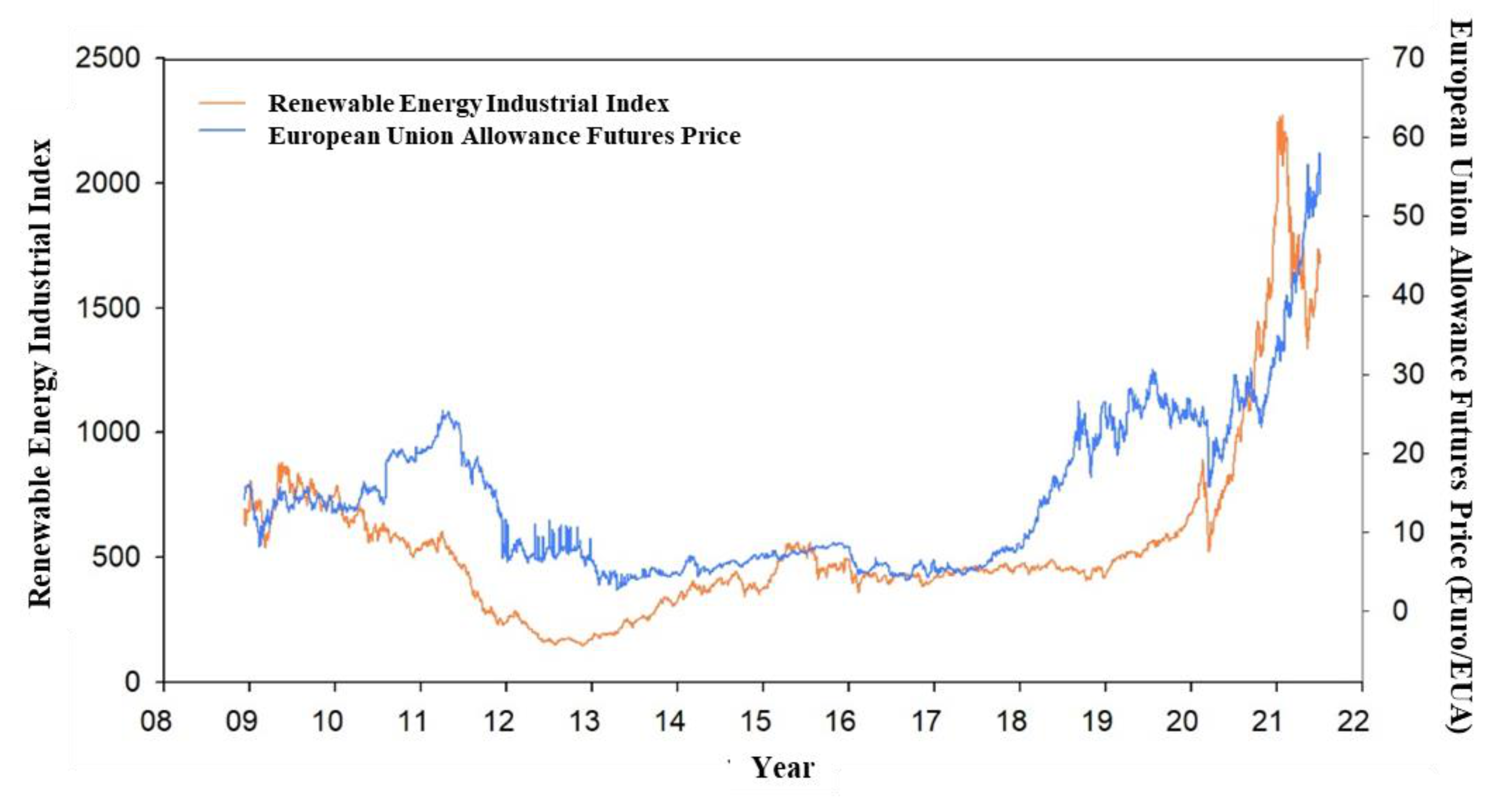
2.1. Data
2.2. Methods
3. Empirical Results
3.1. Return Spillover Table
3.1.1. “Carbon–Renewable Energy–Finance–Energy” Market System
3.1.2. “Carbon–Renewable Energy–Finance” and “Carbon–Renewable Energy–Energy” Market Systems
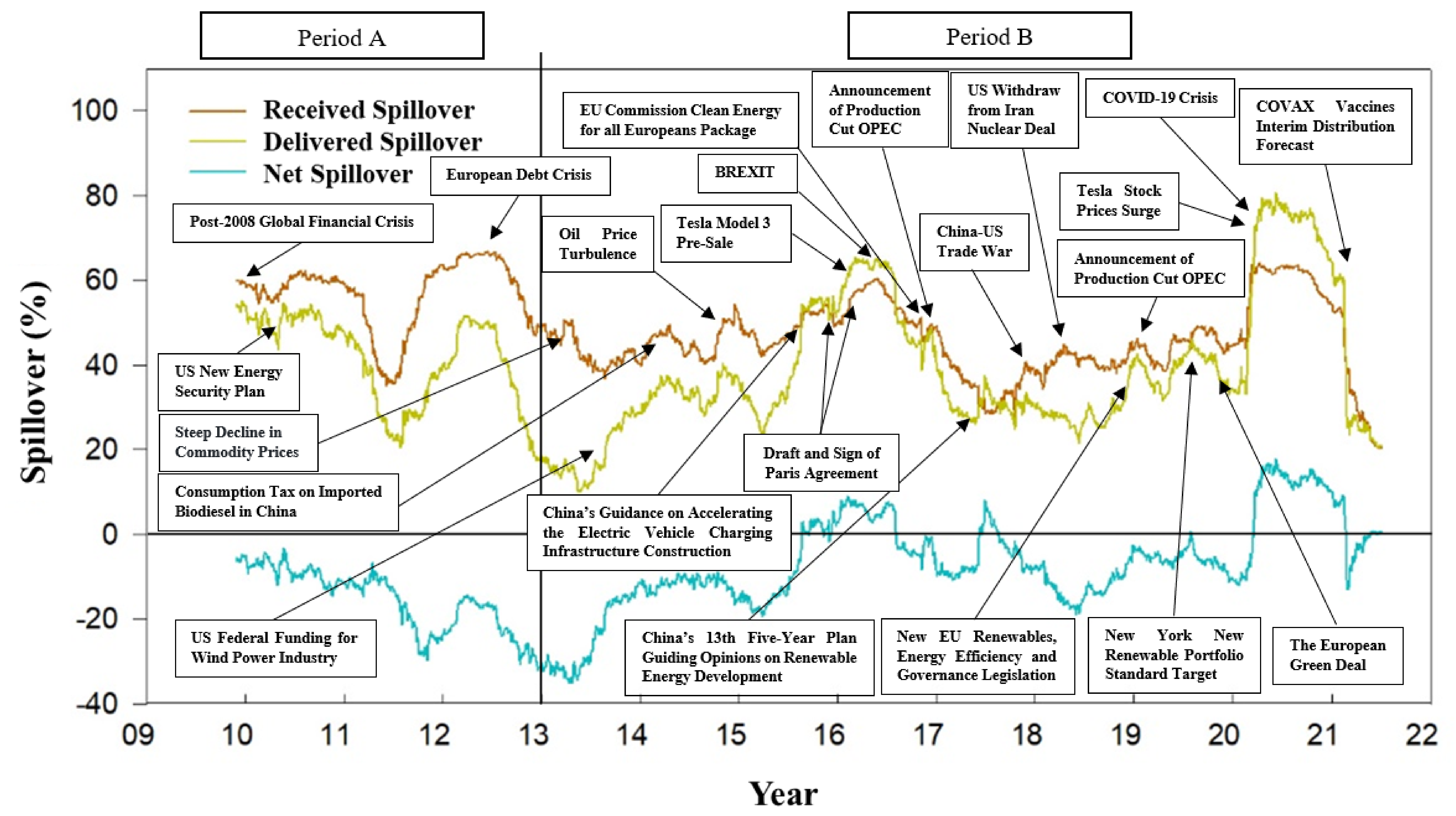
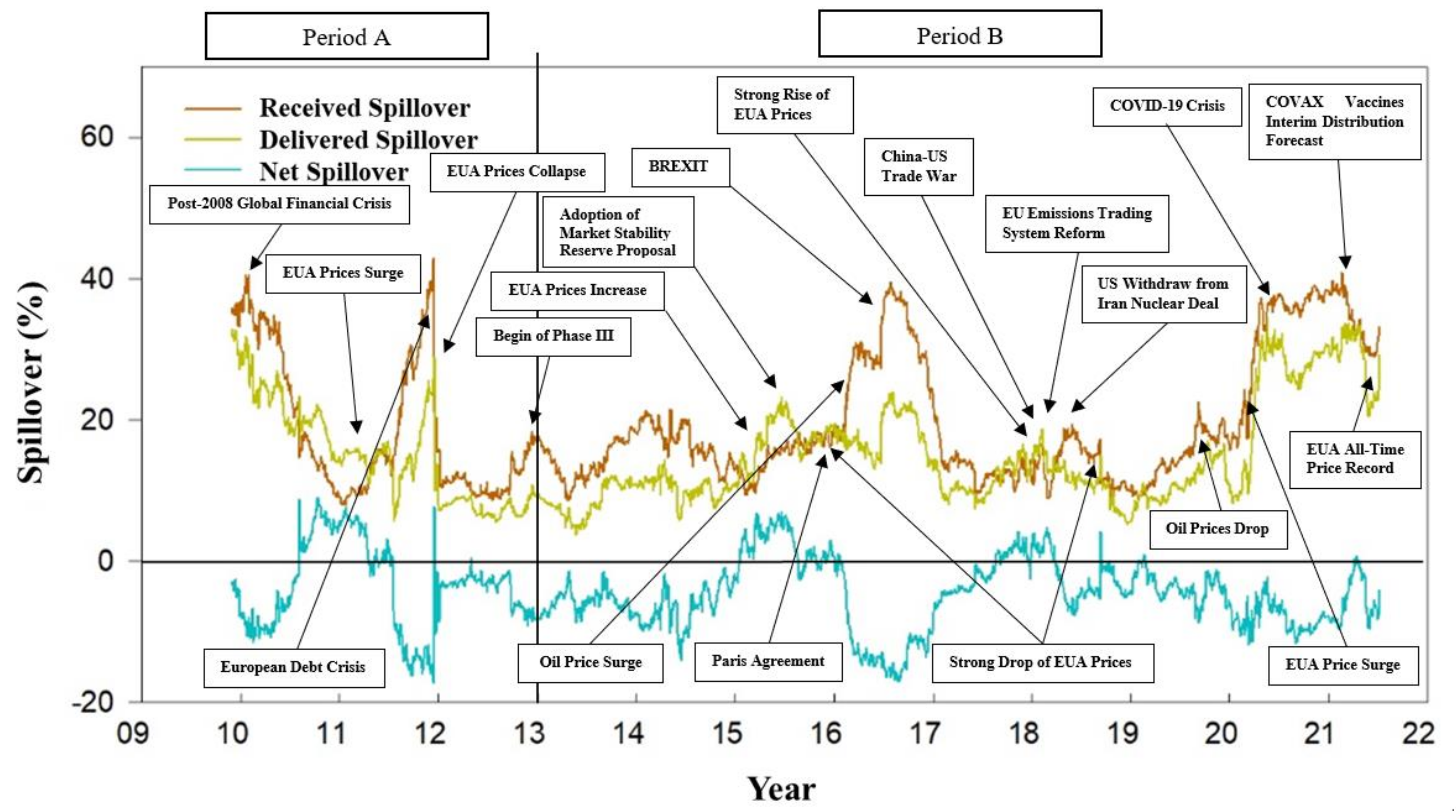
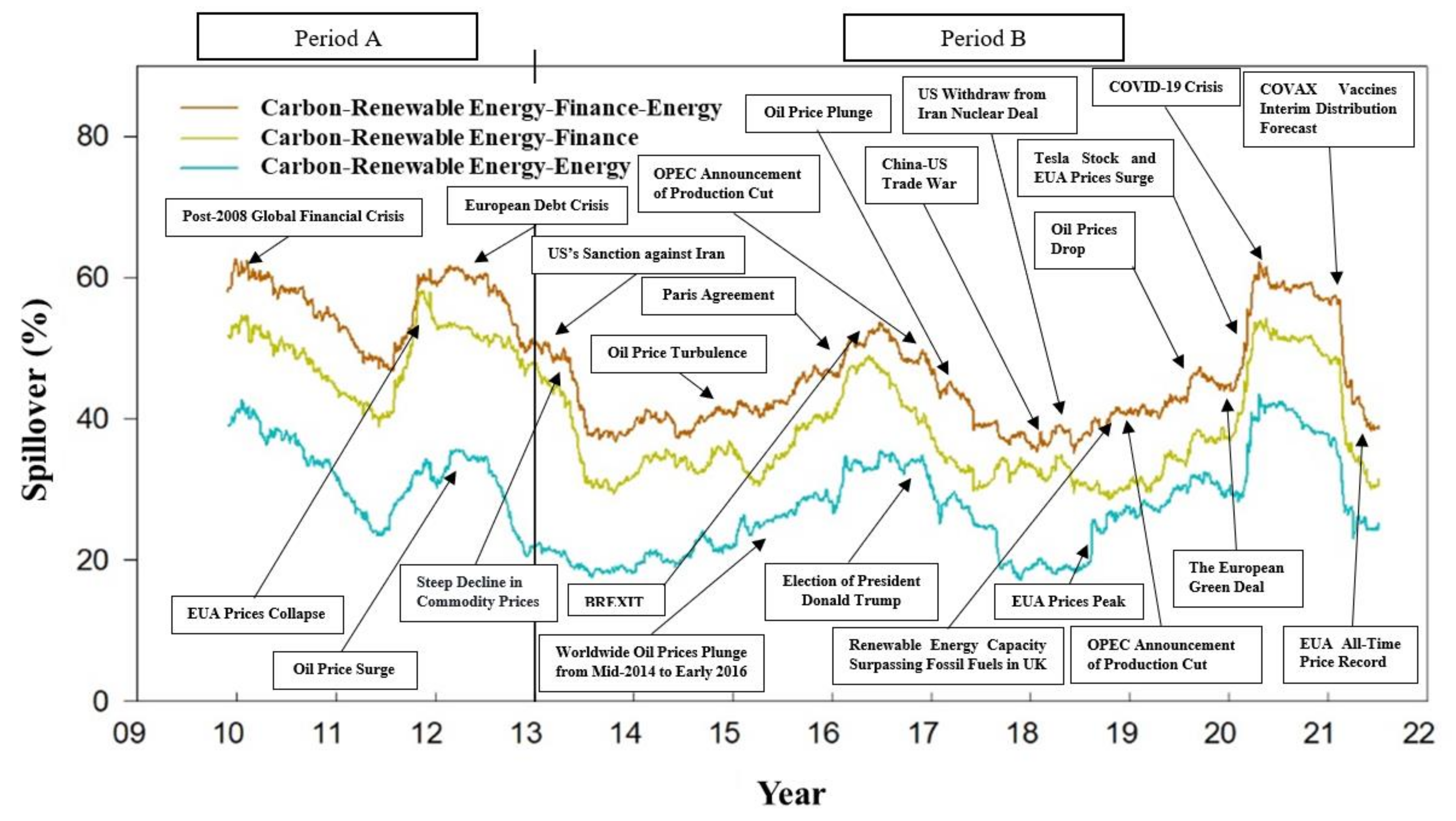
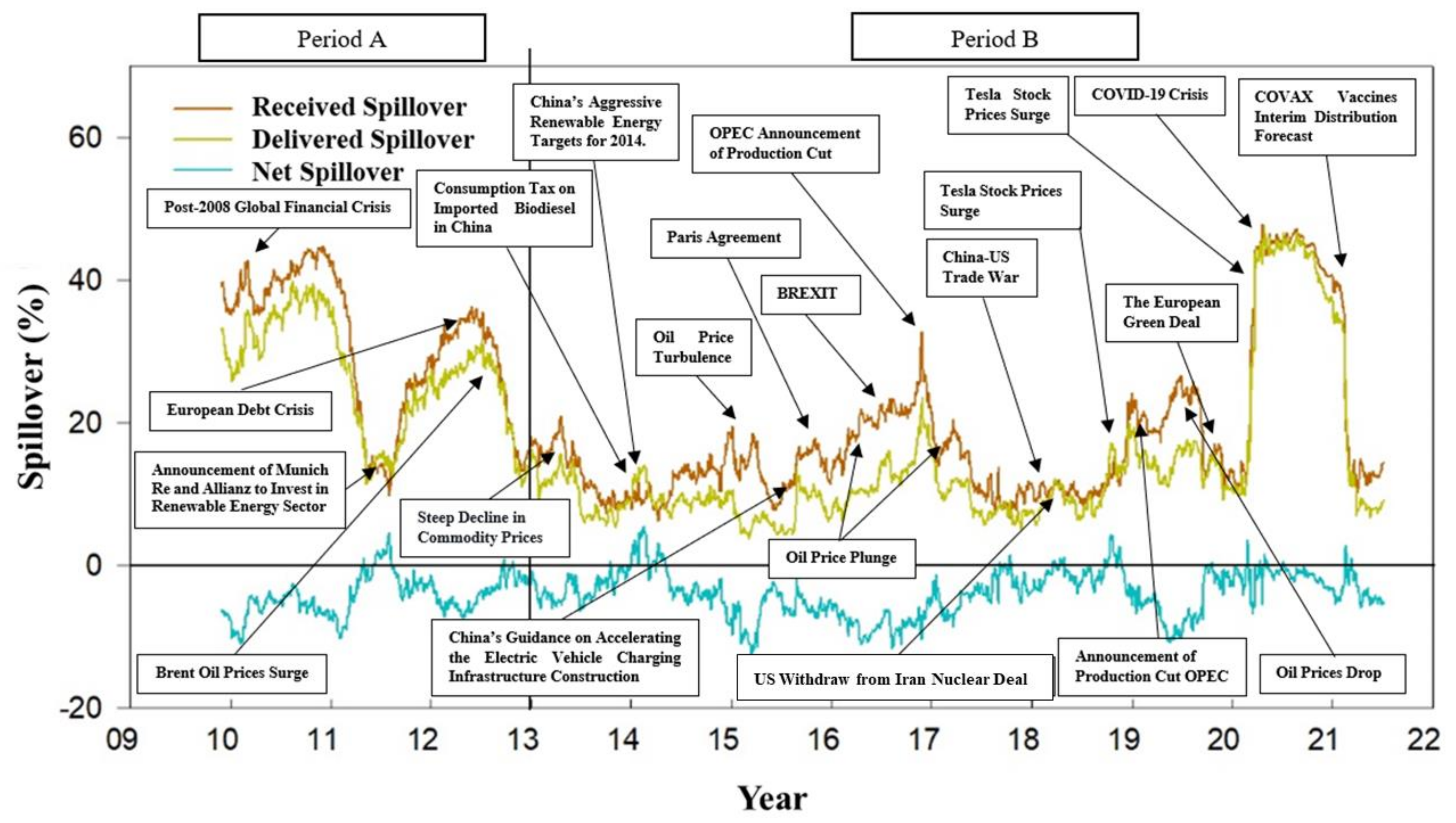
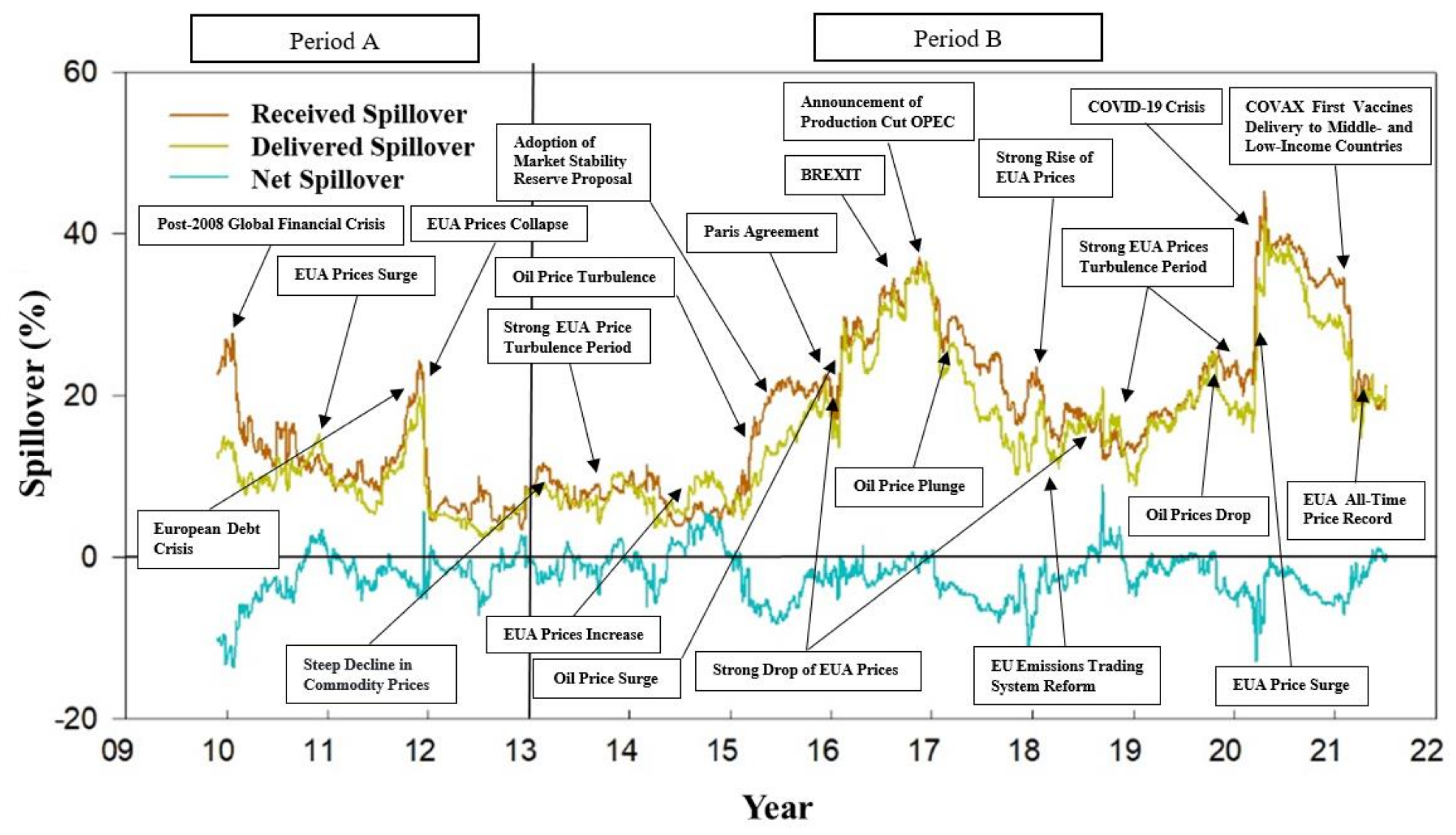
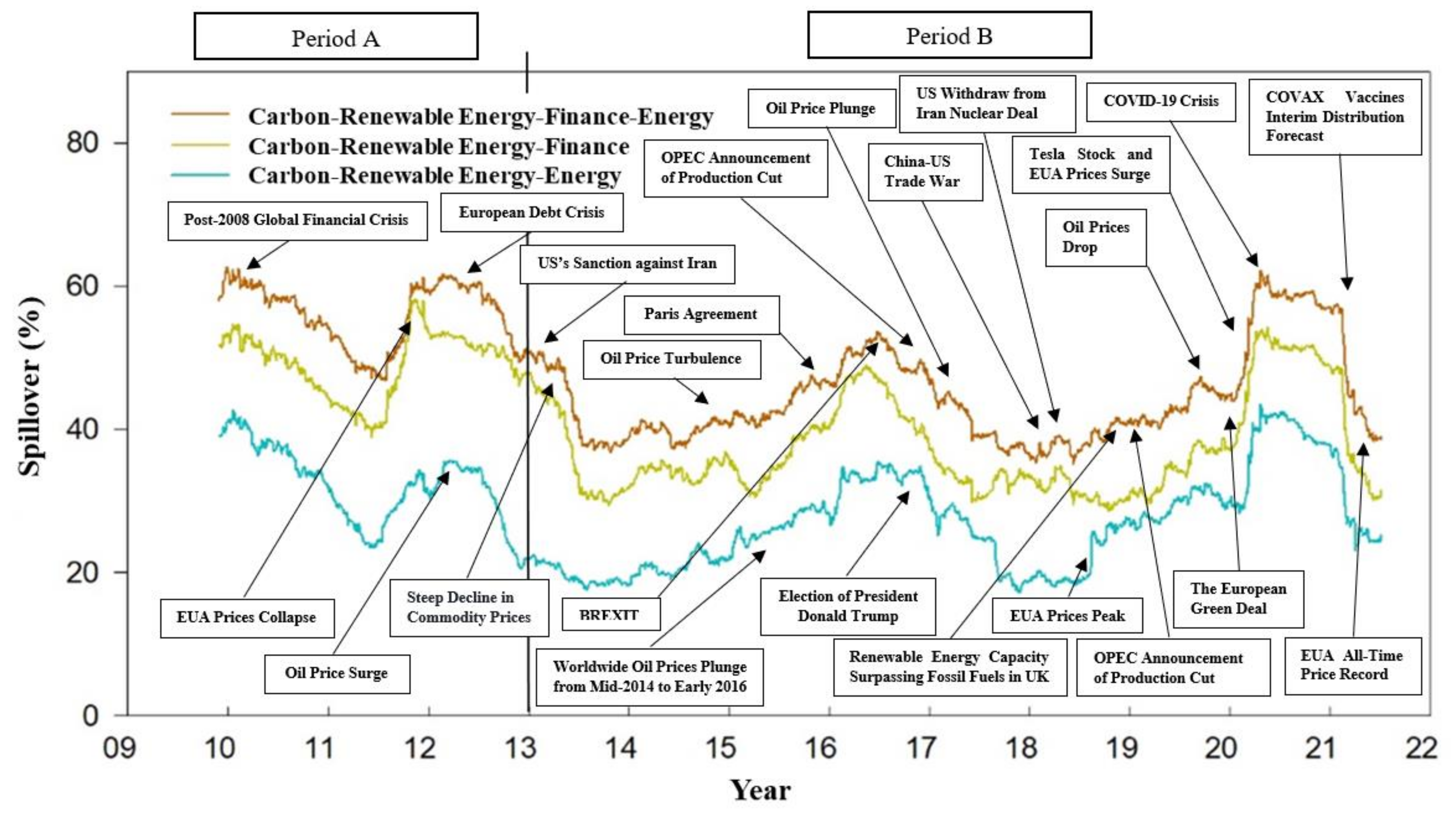
3.2. Return Spillover Plot
4. Robustness Check
5. Discussion
6. Conclusions
Author Contributions
Funding
Data Availability Statement
Acknowledgments
Conflicts of Interest
Appendix A

| Company | HQ | Branch | ISIN | Weight |
|---|---|---|---|---|
| Albioma | FRA | Wind and Solar Energy | FR0000060402 | 0.52% |
| Ballard Power Systems | CAN | Fuel Cell | CA0585861085 | 2.91% |
| Canadian Solar | CAN | Solar Energy | CA1366351098 | 1.14% |
| China Longyuan Power | CHN | Wind Power | CNE100000HD4 | 2.22% |
| Daqo New Energy | CHN | Solar Energy | US23703Q2030 | 2.31% |
| EDP Renováveis | ESP | Wind Power | ES0127797019 | 1.66% |
| ENCAVIS | GER | Wind and Solar Energy | DE0006095003 | 0.98% |
| Enphase Energy | USA | Solar Energy | US29355A1079 | 9.12% |
| First Solar | USA | Solar Energy | US3364331070 | 4.09% |
| Innergex Renewable Energy | USA | Hydro, Wind and Solar Energy | CA45790B1040 | 1.15% |
| ITM Power | GBR | Electrolysers | GB00B0130H42 | 1.16% |
| Jinko Solar | CHN | Solar Energy | US47759T1007 | 0.95% |
| Nel | NOR | Fuel Cell | NO0010081235 | 1.18% |
| Neoen | FRA | Wind and Solar Energy | FR0011675362 | 0.79% |
| Nordex | GER | Wind Power | DE000A0D6554 | 1.27% |
| Ormat Technologies | USA | Geothermal Power | US6866881021 | 1.00% |
| Ørsted | DNK | Wind Power | DK0060094928 | 10.00% |
| Plug Power | USA | Fuel Cell | US72919P2020 | 7.89% |
| PowerCell | SWE | Fuel Cell | SE0006425815 | 0.71% |
| Scatec | NOR | Solar Energy | NO0010715139 | 1.52% |
| Siemens Gamesa | ESP | Wind Power | ES0143416115 | 4.43% |
| SolarEdge | ISR | Solar Energy | US83417M1045 | 7.26% |
| Sunnova Energy | USA | Solar Energy | US86745K1043 | 1.55% |
| SunPower | USA | Solar Energy | US8676524064 | 1.32% |
| Sunrun | USA | Solar Energy | US86771W1053 | 5.94% |
| Tesla | USA | Electric Vehicle | US88160R1014 | 10.00% |
| Verbund | AUT | Hydropower | AT0000746409 | 2.41% |
| Vestas | DNK | Wind Power | DK0061539921 | 10.00% |
| Goldwind | CHN | Wind Power | CNE100000PP1 | 0.73% |
| Xinyi Solar | CHN | Solar Energy | KYG9829N1025 | 3.80% |
| From | |||||||||||||
|---|---|---|---|---|---|---|---|---|---|---|---|---|---|
| To | Financial | Energy | Emerging | Received Spillover | |||||||||
| ES | US | EB | UB | CY | FX | CO | GE | NG | CL | RE | CE | ||
| Panel A: Short-Term 2-Day-Ahead Forecast Window | |||||||||||||
| ES | 42.86 | 20.60 | 0.10 | 7.10 | 4.50 | 0.88 | 5.13 | 4.03 | 0.17 | 1.26 | 12.75 | 0.61 | 57.14 |
| US | 18.87 | 41.45 | 0.02 | 8.80 | 4.44 | 2.12 | 6.41 | 6.25 | 0.23 | 1.15 | 9.76 | 0.51 | 58.55 |
| EB | 0.83 | 0.11 | 91.18 | 6.34 | 0.15 | 0.64 | 0.06 | 0.07 | 0.11 | 0.15 | 0.35 | 0.01 | 8.82 |
| UB | 9.67 | 12.68 | 3.77 | 58.36 | 1.26 | 0.01 | 4.66 | 4.43 | 0.27 | 0.44 | 4.22 | 0.22 | 41.64 |
| CY | 6.42 | 6.78 | 0.17 | 1.34 | 62.49 | 5.29 | 7.04 | 4.41 | 0.94 | 1.68 | 3.07 | 0.37 | 37.51 |
| FX | 1.56 | 4.31 | 0.18 | 0.05 | 6.91 | 82.97 | 1.36 | 0.67 | 0.37 | 1.16 | 0.08 | 0.39 | 17.03 |
| CO | 5.35 | 7.05 | 0.03 | 3.52 | 5.17 | 0.74 | 45.58 | 25.29 | 0.63 | 2.89 | 3.12 | 0.63 | 54.42 |
| GE | 4.52 | 7.25 | 0.00 | 3.51 | 3.42 | 0.40 | 26.97 | 48.55 | 0.53 | 1.51 | 2.89 | 0.45 | 51.45 |
| NG | 0.38 | 0.53 | 0.08 | 0.54 | 1.34 | 0.57 | 1.36 | 1.01 | 93.52 | 0.19 | 0.32 | 0.15 | 6.48 |
| CL | 2.45 | 2.81 | 0.09 | 0.74 | 2.65 | 1.43 | 5.04 | 2.50 | 0.16 | 78.91 | 1.83 | 1.38 | 21.09 |
| RE | 16.45 | 15.76 | 0.19 | 4.00 | 3.03 | 0.03 | 3.88 | 3.36 | 0.23 | 1.08 | 51.56 | 0.45 | 48.45 |
| CE | 1.29 | 1.02 | 0.01 | 0.31 | 0.50 | 0.37 | 1.22 | 0.84 | 0.15 | 1.72 | 0.75 | 91.82 | 8.18 |
| Delivered Spillover | 67.81 | 78.90 | 4.63 | 36.25 | 33.37 | 12.48 | 63.13 | 52.87 | 3.80 | 13.22 | 39.14 | 5.18 | Total Spillover |
| Net Spillover | 10.67 | 20.35 | −4.19 | −5.39 | −4.15 | −4.55 | 8.71 | 1.41 | −2.68 | −7.87 | −9.30 | −3.01 | 34.23 |
| Panel B: Long-Term 10-Day-Ahead Forecast Window | |||||||||||||
| ES | 42.06 | 20.47 | 0.15 | 7.26 | 4.59 | 1.17 | 5.29 | 4.09 | 0.31 | 1.31 | 12.66 | 0.63 | 57.94 |
| US | 18.66 | 40.53 | 0.28 | 8.83 | 4.44 | 2.50 | 6.55 | 6.33 | 0.41 | 1.17 | 9.78 | 0.52 | 59.47 |
| EB | 1.08 | 0.42 | 87.35 | 7.24 | 0.36 | 1.05 | 0.50 | 0.52 | 0.22 | 0.19 | 0.70 | 0.37 | 12.65 |
| UB | 9.64 | 12.78 | 3.87 | 57.31 | 1.36 | 0.16 | 5.10 | 4.42 | 0.39 | 0.48 | 4.23 | 0.25 | 42.69 |
| CY | 6.50 | 6.81 | 0.53 | 1.59 | 61.10 | 5.31 | 7.07 | 4.41 | 1.19 | 1.75 | 3.26 | 0.49 | 38.90 |
| FX | 1.71 | 4.35 | 0.29 | 0.22 | 6.94 | 81.65 | 1.36 | 0.76 | 0.72 | 1.23 | 0.29 | 0.50 | 18.35 |
| CO | 5.57 | 7.31 | 0.22 | 3.96 | 5.13 | 0.86 | 44.56 | 24.96 | 0.67 | 2.89 | 3.23 | 0.63 | 55.44 |
| GE | 5.14 | 7.49 | 0.20 | 4.21 | 3.39 | 0.58 | 26.33 | 46.92 | 0.61 | 1.50 | 3.18 | 0.47 | 53.08 |
| NG | 0.47 | 0.85 | 0.21 | 0.73 | 1.42 | 0.67 | 1.73 | 1.17 | 91.36 | 0.39 | 0.68 | 0.31 | 8.64 |
| CL | 2.55 | 2.84 | 0.23 | 0.85 | 2.82 | 1.49 | 5.31 | 2.60 | 0.23 | 77.49 | 2.13 | 1.46 | 22.51 |
| RE | 16.21 | 15.75 | 0.33 | 4.10 | 3.10 | 0.18 | 4.25 | 3.52 | 0.34 | 1.19 | 50.50 | 0.54 | 49.50 |
| CE | 1.60 | 1.11 | 0.35 | 0.59 | 0.90 | 0.58 | 1.38 | 0.94 | 0.28 | 1.78 | 0.90 | 89.58 | 10.42 |
| Delivered Spillover | 69.13 | 80.19 | 6.66 | 39.57 | 34.44 | 14.56 | 64.88 | 53.73 | 5.36 | 13.87 | 41.04 | 6.16 | Total Spillover |
| Net Spillover | 11.19 | 20.72 | −5.99 | −3.11 | −4.46 | −3.79 | 9.44 | 0.65 | −3.28 | −8.64 | −8.46 | −4.25 | 34.23 |
| From | |||||||||
|---|---|---|---|---|---|---|---|---|---|
| To | Financial | Emerging | Received Spillover | ||||||
| ES | US | EB | UB | CY | FX | RE | CE | ||
| Panel A: Short-Term 2-Day-Ahead Forecast Window | |||||||||
| ES | 47.64 | 22.96 | 0.10 | 8.09 | 5.13 | 0.95 | 14.43 | 0.70 | 52.36 |
| US | 21.93 | 47.92 | 0.03 | 10.46 | 5.22 | 2.49 | 11.33 | 0.61 | 52.08 |
| EB | 0.75 | 0.08 | 91.69 | 6.32 | 0.16 | 0.66 | 0.33 | 0.02 | 8.31 |
| UB | 10.89 | 14.32 | 4.12 | 64.06 | 1.53 | 0.02 | 4.79 | 0.27 | 35.94 |
| CY | 7.65 | 7.99 | 0.19 | 1.73 | 72.25 | 5.99 | 3.72 | 0.48 | 27.75 |
| FX | 1.57 | 4.53 | 0.21 | 0.03 | 7.05 | 86.13 | 0.06 | 0.42 | 13.87 |
| RE | 18.18 | 17.15 | 0.17 | 4.51 | 3.39 | 0.03 | 56.05 | 0.52 | 43.95 |
| CE | 1.38 | 1.11 | 0.01 | 0.35 | 0.58 | 0.38 | 0.83 | 95.37 | 4.63 |
| Delivered Spillover | 62.36 | 68.14 | 4.83 | 31.50 | 23.06 | 10.51 | 35.50 | 3.02 | Total Spillover |
| Net Spillover | 10.00 | 16.05 | −3.49 | −4.45 | −4.69 | −3.36 | −8.45 | −1.62 | 29.86 |
| Panel B: Short-Term 5-Day-Ahead Forecast Window | |||||||||
| ES | 47.41 | 22.94 | 0.13 | 8.12 | 5.13 | 1.10 | 14.49 | 0.70 | 52.59 |
| US | 21.99 | 47.47 | 0.19 | 10.37 | 5.26 | 2.63 | 11.48 | 0.61 | 52.53 |
| EB | 0.83 | 0.14 | 90.92 | 6.41 | 0.30 | 0.68 | 0.48 | 0.24 | 9.08 |
| UB | 10.97 | 14.53 | 4.14 | 63.64 | 1.58 | 0.04 | 4.81 | 0.29 | 36.36 |
| CY | 7.77 | 8.03 | 0.44 | 1.88 | 71.56 | 5.96 | 3.82 | 0.54 | 28.44 |
| FX | 1.67 | 4.53 | 0.27 | 0.19 | 7.14 | 85.56 | 0.17 | 0.47 | 14.44 |
| RE | 18.15 | 17.08 | 0.31 | 4.54 | 3.41 | 0.08 | 55.88 | 0.55 | 44.12 |
| CE | 1.51 | 1.14 | 0.09 | 0.35 | 0.78 | 0.47 | 0.90 | 94.75 | 5.25 |
| Delivered Spillover | 62.90 | 68.38 | 5.57 | 31.85 | 23.60 | 10.95 | 36.15 | 3.40 | Total Spillover |
| Net Spillover | 10.31 | 15.85 | −3.51 | −4.50 | −4.84 | −3.49 | −7.97 | −1.85 | 30.35 |
| Panel C: Long-Term 10-Day-Ahead Forecast Window | |||||||||
| ES | 46.96 | 22.95 | 0.16 | 8.30 | 5.23 | 1.28 | 14.38 | 0.72 | 53.04 |
| US | 21.83 | 47.09 | 0.33 | 10.52 | 5.24 | 2.96 | 11.40 | 0.63 | 52.91 |
| EB | 1.00 | 0.42 | 88.79 | 7.29 | 0.35 | 1.07 | 0.70 | 0.38 | 11.21 |
| UB | 10.96 | 14.60 | 4.29 | 63.22 | 1.62 | 0.20 | 4.82 | 0.29 | 36.78 |
| CY | 7.77 | 8.04 | 0.58 | 1.98 | 71.00 | 6.04 | 3.96 | 0.63 | 29.00 |
| FX | 1.72 | 4.60 | 0.32 | 0.21 | 7.12 | 85.19 | 0.29 | 0.54 | 14.81 |
| RE | 18.06 | 17.29 | 0.33 | 4.67 | 3.49 | 0.19 | 55.34 | 0.62 | 44.66 |
| CE | 1.72 | 1.22 | 0.37 | 0.66 | 1.00 | 0.61 | 1.00 | 93.43 | 6.57 |
| Delivered Spillover | 110.03 | 116.21 | 95.17 | 96.86 | 95.05 | 97.54 | 91.89 | 97.25 | Total Spillover |
| Net Spillover | 10.03 | 16.21 | −4.83 | −3.14 | −4.95 | −2.46 | −8.11 | −2.75 | 31.12 |
| From | Received Spillover | ||||||
|---|---|---|---|---|---|---|---|
| Energy | Emerging | ||||||
| To | CO | GE | NG | CL | RE | CE | |
| Panel A: Short-Term 2-Day-Ahead Forecast Window | |||||||
| CO | 58.72 | 31.76 | 0.80 | 3.85 | 4.05 | 0.82 | 41.28 |
| GE | 32.63 | 60.30 | 0.65 | 1.97 | 3.83 | 0.62 | 39.70 |
| NG | 1.41 | 1.05 | 96.86 | 0.19 | 0.33 | 0.16 | 3.14 |
| CL | 5.78 | 2.87 | 0.17 | 87.13 | 2.46 | 1.60 | 12.87 |
| RE | 6.36 | 5.71 | 0.35 | 2.21 | 84.59 | 0.79 | 15.41 |
| CE | 1.28 | 0.95 | 0.16 | 1.89 | 0.83 | 94.89 | 5.11 |
| Delivered Spillover | 47.45 | 42.34 | 2.12 | 10.11 | 11.49 | 3.99 | Total Spillover |
| Net Spillover | 6.17 | 2.64 | −1.01 | −2.76 | −3.92 | −1.12 | 19.59 |
| Panel B: Short-Term 5-Day-Ahead Forecast Window | |||||||
| CO | 58.45 | 31.86 | 0.83 | 3.86 | 4.16 | 0.84 | 41.55 |
| GE | 32.75 | 59.92 | 0.67 | 1.99 | 4.05 | 0.63 | 40.08 |
| NG | 1.76 | 1.25 | 96.17 | 0.20 | 0.39 | 0.24 | 3.83 |
| CL | 5.84 | 2.90 | 0.24 | 86.69 | 2.67 | 1.66 | 13.31 |
| RE | 6.62 | 5.72 | 0.42 | 2.40 | 84.02 | 0.83 | 15.98 |
| CE | 1.35 | 1.06 | 0.20 | 1.92 | 0.89 | 94.58 | 5.42 |
| Delivered Spillover | 48.31 | 42.80 | 2.36 | 10.35 | 12.16 | 4.19 | Total Spillover |
| Net Spillover | 6.76 | 2.72 | −1.47 | −2.96 | −3.82 | −1.23 | 20.03 |
| Panel C: Long-Term 10-Day-Ahead Forecast Window | |||||||
| CO | 58.26 | 31.88 | 0.88 | 3.91 | 4.23 | 0.84 | 41.74 |
| GE | 32.72 | 59.77 | 0.77 | 1.98 | 4.11 | 0.64 | 40.23 |
| NG | 1.81 | 1.24 | 95.68 | 0.36 | 0.63 | 0.27 | 4.32 |
| CL | 6.13 | 2.97 | 0.25 | 86.25 | 2.71 | 1.69 | 13.75 |
| RE | 6.98 | 6.02 | 0.52 | 2.42 | 83.18 | 0.89 | 16.82 |
| CE | 1.39 | 1.07 | 0.28 | 1.92 | 0.98 | 94.36 | 5.64 |
| Delivered Spillover | 49.04 | 43.19 | 2.69 | 10.59 | 12.65 | 4.34 | Total Spillover |
| Net Spillover | 7.30 | 2.96 | −1.63 | −3.16 | −4.17 | −1.30 | 20.42 |
References
- Arshanapalli, B.; Doukas, J. International Stock Market Linkages: Evidence From the Pre- and Post-October 1987 Period. J. Bank. Financ. 1993, 17, 193–208. [Google Scholar] [CrossRef]
- Eun, C.S.; Shim, S. International Transmission of Stock Market Movements. J. Financ. Quant. Anal. 1989, 24, 241–256. [Google Scholar] [CrossRef]
- Jeon, B.N.; Furstenberg, G.M.V. Growing International Co-Movement in Stock Price Indexes. Q. Rev. Econ. Bus. 1990, 30, 15–31. [Google Scholar]
- King, M.A.; Wadhwani, S. Transmission of Volatility between Stock Markets. Rev. Financ. Stud. 1990, 3, 5–33. [Google Scholar] [CrossRef]
- King, M.; Sentana, E.; Wadhwani, S. Volatility and Links between National Stock Markets. Econometrica 1994, 62, 901–933. [Google Scholar] [CrossRef]
- Koutmos, G.; Booth, G.G. Asymmetric Volatility Transmission in International Stock Markets. J. Int. Money Financ. 1995, 14, 747–762. [Google Scholar] [CrossRef]
- Longin, F.; Solnik, B. Is the Correlation in International Equity Returns Constant: 1960–1990? J. Int. Money Financ. 1995, 14, 3–26. [Google Scholar] [CrossRef]
- Schöllhammer, H.; Sand, O. The Interdependece among the Stock Markets of Major European Countries and the United States: An Empirical Investigation of Interrelationships among National Stock Price Movements. Manag. Int. Rev. 1985, 25, 17–26. [Google Scholar]
- Taylor, M.P.; Tonks, I. The Internationalisation of Stock Markets and the Abolition of U.K. Exchange Control. Rev. Econ. Stat. 1989, 71, 332–336. [Google Scholar] [CrossRef]
- Bekaert, G.; Harvey, C.R. Time-Varying World Market Integration. J. Financ. 1995, 50, 403–444. [Google Scholar] [CrossRef]
- Bekaert, G.; Harvey, C.R. Market Integration and Contagion. In Working Paper Series; National Bureau of Economic Research: Cambridge, MA, USA, 2003. [Google Scholar]
- Abbas, G.; Hammoudeh, S.; Shahzad, S.J.H.; Wang, S.; Wei, Y. Return and Volatility Connectedness between Stock Markets and Macroeconomic Factors in the G-7 Countries. J. Syst. Sci. Syst. Eng. 2019, 28, 1–36. [Google Scholar] [CrossRef]
- Dungey, M.; Martin, V.L. Unravelling Financial Market Linkages during Crises. J. Appl. Econom. 2007, 22, 89–119. [Google Scholar] [CrossRef]
- Guimarães-Filho, R.; Hong, G.H. Dynamic Connectedness of Asian Equity Markets; International Monetary Fund: Washington, DC, USA, 2016; Volume 16, pp. 1–36. [Google Scholar]
- Zhou, X.; Zhang, W.; Zhang, J. Volatility Spillovers between the Chinese and World Equity Markets. Pac. Basin Financ. J. 2012, 20, 247–270. [Google Scholar] [CrossRef]
- Bekaert, G.; Harvey, C.R.; Lundblad, C.; Siegel, S. Global Growth Opportunities and Market Integration. J. Financ. 2007, 62, 1081–1137. [Google Scholar] [CrossRef]
- Forbes, K.J.; Rigobon, R. No Contagion, Only Interdependence: Measuring Stock Market Comovements. J. Financ. 2002, 57, 2223–2261. [Google Scholar] [CrossRef]
- Gulzar, S.; Kayani, G.M.; Xiaofeng, H.; Ayub, U.; Rafique, A. Financial Cointegration and Spillover Effect of Global Financial Crisis: A Study of Emerging Asian Financial Markets. Econ. Res. Ekon. 2019, 32, 187–218. [Google Scholar] [CrossRef] [Green Version]
- Masih, A.M.M.; Masih, R. Dynamic Linkages and the Propagation Mechanism Driving Major International Stock Markets: An Analysis of the Pre- and Post-Crash Eras. Q. Rev. Econ. Financ. 1997, 37, 859–885. [Google Scholar] [CrossRef]
- Tuluca, S.A.; Zwick, B. The Effects of the Asian Crisis on Global Equity Markets. Financ. Rev. 2001, 36, 125–142. [Google Scholar] [CrossRef]
- Levine, R. Financial Development and Economic Growth: Views and Agenda. J. Econ. Lit. 1997, 35, 688–726. [Google Scholar]
- Kose, M.A.; Prasad, E.; Rogoff, K.; Wei, S.-J. Financial Globalization: A Reappraisal. IMF Staff Pap. 2009, 56, 8–62. [Google Scholar] [CrossRef] [Green Version]
- Lewis, K.K. Trying to Explain Home Bias in Equities and Consumption. J. Econ. Lit. 1999, 37, 571–608. [Google Scholar] [CrossRef] [Green Version]
- Obstfeld, M. Risk-Taking, Global Diversification, and Growth. Am. Econ. Rev. 1994, 84, 1310–1329. [Google Scholar]
- Van Wincoop, E. How Big Are Potential Welfare Gains from International Risksharing? J. Int. Econ. 1999, 47, 109–135. [Google Scholar] [CrossRef] [Green Version]
- Ajadi, T.; Boyle, R.; Strahan, D.; Kimmel, M.; Collins, B.; Cheung, A.; Becker, L. Global Trends in Renewable Energy Investment 2020; Frankfurt School-UNEP Centre/BNEF: Frankfurt, Germany, 2020; Available online: https://www.fs-unep-centre.org/wp-content/uploads/2020/06/GTR_2020.pdf (accessed on 16 July 2021).
- Valuates Reportes. Renewable Energy Market Size, Share, Growth, Industry Analysis, Report; Bangalore, India, 2019. Available online: https://www.openpr.com/news/2409952/renewable-energy-market-size-worth-over-1-977-6-billion-by-2030 (accessed on 16 July 2021).
- Lecocq, F. State and Trends of the Carbon Market 2004. In World Bank Working Papers; The World Bank: Washington, DC, USA, 2005. [Google Scholar]
- Berntsen, J.; Fjellheim, H.; Maria, K.; Cathy, L.; Rihel, A.S.; Zelljadt, E. Carbon Market Year in Review 2020; Refinitiv: London, UK, 2021; Available online: https://www.refinitiv.com/content/dam/marketing/en_us/documents/reports/carbon-market-year-in-review-2020.pdf (accessed on 19 July 2021).
- Mansanet-Bataller, M.; Soriano, P. Volatility Transmission in the CO2 and Energy Markets. In Proceedings of the 2009 6th International Conference on the European Energy Market, Leuven, Belgium, 27–29 May 2009; pp. 1–7. [Google Scholar]
- Aatola, P.; Ollikainen, M.; Toppinen, A. Impact of the Carbon Price on the Integrating European Electricity Market. Energy Policy 2013, 61, 1236–1251. [Google Scholar] [CrossRef]
- Boersen, A.; Scholtens, B. The Relationship between European Electricity Markets and Emission Allowance Futures Prices in Phase II of the EU (European Union) Emission Trading Scheme. Energy 2014, 74, 585–594. [Google Scholar] [CrossRef]
- Chen, Y.; Qu, F.; Li, W.; Chen, M. Volatility Spillover and Dynamic Correlation between the Carbon Market and Energy Markets. J. Bus. Econ. Manag. 2019, 20, 979–999. [Google Scholar] [CrossRef] [Green Version]
- Dhamija, A.K.; Yadav, S.S.; Jain, P. Forecasting Volatility of Carbon under EU ETS: A Multi-Phase Study. Environ. Econ. Policy Stud. 2017, 19, 299–335. [Google Scholar] [CrossRef]
- Hammoudeh, S.; Lahiani, A.; Nguyen, D.K.; Sousa, R.M. An Empirical Analysis of Energy Cost Pass-through to CO2 Emission Prices. Energy Econ. 2015, 49, 149–156. [Google Scholar] [CrossRef]
- Ji, Q.; Zhang, D.; Geng, J. Information Linkage, Dynamic Spillovers in Prices and Volatility between the Carbon and Energy Markets. J. Clean. Prod. 2018, 198, 972–978. [Google Scholar] [CrossRef]
- Kanamura, T. Role of Carbon Swap Trading and Energy Prices in Price Correlations and Volatilities between Carbon Markets. Energy Econ. 2016, 54, 204–212. [Google Scholar] [CrossRef]
- Keppler, J.H.; Mansanet-Bataller, M. Causalities between CO2, Electricity, and Other Energy Variables during Phase I and Phase II of the EU ETS. Energy Policy 2010, 38, 3329–3341. [Google Scholar] [CrossRef] [Green Version]
- Reboredo, J.C. Volatility Spillovers between the Oil Market and the European Union Carbon Emission Market. Econ. Model. 2014, 36, 229–234. [Google Scholar] [CrossRef]
- Wang, Y.; Guo, Z. The Dynamic Spillover between Carbon and Energy Markets: New Evidence. Energy 2018, 149, 24–33. [Google Scholar] [CrossRef]
- Chevallier, J. Macroeconomics, Finance, Commodities: Interactions with Carbon Markets in a Data-Rich Model. Econ. Model. 2011, 28, 557–567. [Google Scholar] [CrossRef] [Green Version]
- Creti, A.; Jouvet, P.-A.; Mignon, V. Carbon Price Drivers: Phase I versus Phase II Equilibrium? Energy Econ. 2012, 34, 327–334. [Google Scholar] [CrossRef] [Green Version]
- Kumar, S.; Managi, S.; Matsuda, A. Stock Prices of Clean Energy Firms, Oil and Carbon Markets: A Vector Autoregressive Analysis. Energy Econ. 2012, 34, 215–226. [Google Scholar] [CrossRef]
- Oestreich, A.M.; Tsiakas, I. Carbon Emissions and Stock Returns: Evidence from the EU Emissions Trading Scheme. J. Bank. Financ. 2015, 58, 294–308. [Google Scholar] [CrossRef]
- Tian, Y.; Akimov, A.; Roca, E.; Wong, V. Does the Carbon Market Help or Hurt the Stock Price of Electricity Companies? Further Evidence from the European Context. J. Clean. Prod. 2016, 112, 1619–1626. [Google Scholar] [CrossRef] [Green Version]
- Koch, N. Dynamic Linkages among Carbon, Energy and Financial Markets: A Smooth Transition Approach. Appl. Econ. 2014, 46, 715–729. [Google Scholar] [CrossRef]
- Tan, X.; Sirichand, K.; Vivian, A.; Wang, X. How Connected Is the Carbon Market to Energy and Financial Markets? A Systematic Analysis of Spillovers and Dynamics. Energy Econ. 2020, 90, 104870. [Google Scholar] [CrossRef]
- Ferrer, R.; Shahzad, S.J.H.; López, R.; Jareño, F. Time and Frequency Dynamics of Connectedness between Renewable Energy Stocks and Crude Oil Prices. Energy Econ. 2018, 76, 1–20. [Google Scholar] [CrossRef]
- Song, Y.; Ji, Q.; Du, Y.-J.; Geng, J.-B. The Dynamic Dependence of Fossil Energy, Investor Sentiment and Renewable Energy Stock Markets. Energy Econ. 2019, 84, 104564. [Google Scholar] [CrossRef]
- Jiang, Y.; Wang, J.; Lie, J.; Mo, B. Dynamic Dependence Nexus and Causality of the Renewable Energy Stock Markets on the Fossil Energy Markets. Energy 2021, 233, 12119. [Google Scholar] [CrossRef]
- Mroua, M.; Bouattour, H.; Naifar, N. Dynamic Links between Renewable Energy, Commodities, and Financial Stock Markets: Implications for Portfolio Diversification. Int. J. Financ. Eng. 2021, 2150023. [Google Scholar] [CrossRef]
- Uddin, G.S.; Rahman, M.L.; Hedström, A.; Ahmed, A. Cross-Quantilogram-Based Correlation and Dependence between Renewable Energy Stock and Other Asset Classes. Energy Econ. 2019, 80, 743–759. [Google Scholar] [CrossRef]
- Kodres, L.E.; Pritsker, M. A Rational Expectations Model of Financial Contagion. J. Financ. 2002, 57, 769–799. [Google Scholar] [CrossRef] [Green Version]
- Diebold, F.X.; Yilmaz, K. Better to Give than to Receive: Predictive Directional Measurement of Volatility Spillovers. Int. J. Forecast. 2012, 28, 57–66. [Google Scholar] [CrossRef] [Green Version]
- Bouri, E.; Cepni, O.; Gabauer, D.; Gupta, R. Return Connectedness across Asset Classes around the COVID-19 Outbreak. Int. Rev. Financ. Anal. 2021, 73, 101646. [Google Scholar] [CrossRef]
- Diebold, F.X.; Yilmaz, K. Measuring Financial Asset Return and Volatility Spillovers, with Application to Global Equity Markets. Econ. J. 2009, 119, 158–171. [Google Scholar] [CrossRef] [Green Version]
- Koop, G.; Pesaran, M.H.; Potter, S.M. Impulse Response Analysis in Nonlinear Multivariate Models. J. Econom. 1996, 74, 119–147. [Google Scholar] [CrossRef]
- Pesaran, H.H.; Shin, Y. Generalized Impulse Response Analysis in Linear Multivariate Models. Econ. Lett. 1998, 58, 17–29. [Google Scholar] [CrossRef]
- Dickey, D.A.; Fuller, W.A. Distribution of the Estimators for Autoregressive Time Series with a Unit Root. J. Am. Stat. Assoc. 1979, 74, 427–431. [Google Scholar]
- Dickey, D.A.; Fuller, W.A. Likelihood Ratio Statistics for Autoregressive Time Series with a Unit Root. Econometrica 1981, 49, 1057–1072. [Google Scholar] [CrossRef]
- Kwiatkowski, D.; Phillips, P.C.B.; Schmidt, P.; Shin, Y. Testing the Null Hypothesis of Stationarity against the Alternative of a Unit Root. J. Econom. 1992, 54, 159–178. [Google Scholar] [CrossRef]
- Jarque, C.M.; Bera, A.K. A Test for Normality of Observations and Regression Residuals. Int. Stat. Rev. 1987, 55, 163–172. [Google Scholar] [CrossRef]
- Graham, M.; Hasselgren, A.; Peltomäki, J. Using CO2 Emission Allowances in Equity Portfolios. In Handbook of Environmental and Sustainable Finance, 1st ed.; Elsevier: Amsterdam, The Netherlands, 2016; pp. 359–370. [Google Scholar]
- Uddin, G.S.; Hernandez, J.A.; Shahzad, S.J.H.; Hedström, A. Multivariate Dependence and Spillover Effects across Energy Commodities and Diversification Potentials of Carbon Assets. Energy Econ. 2018, 71, 35–46. [Google Scholar] [CrossRef]
- Declercq, B.; Delarue, E.; D’haeseleer, W. Impact of the Economic Recession on the European Power Sector’s CO2 Emissions. Energy Policy 2011, 39, 1677–1686. [Google Scholar] [CrossRef]
- Koch, N.; Fuss, S.; Grosjean, G.; Edenhofer, O. Causes of the EU ETS Price Drop: Recession, CDM, Renewable Policies or a Bit of Everything?—New Evidence. Energy Policy 2014, 73, 676–685. [Google Scholar] [CrossRef] [Green Version]
- Benguria, F.; Choi, J.; Swenson, D.L.; Xu, M. Anxiety or Pain? The Impact of Tariffs and Uncertainty on Chinese Firms in the Trade War. In Working Paper Series; National Bureau of Economic Research: Cambridge, MA, USA, 2020. [Google Scholar]
- Grosjean, G.; Acworth, W.; Flachsland, C.; Marschinski, R. After Monetary Policy, Climate Policy: Is Delegation the Key to EU ETS Reform? Clim. Policy 2016, 16, 1–25. [Google Scholar] [CrossRef]
- S&P Global Platts Analysts See EU Carbon Prices at Eur56-Eur89/Mt by 2030. Available online: https://www.spglobal.com/platts/en/market-insights/latest-news/coal/120320-analysts-see-eu-carbon-prices-at-eur56-eur89mt-by-2030 (accessed on 20 August 2021).
- Zheng, Z.; Xiao, R.; Shi, H.; Li, G.; Zhou, X. Statistical Regularities of Carbon Emission Trading Market: Evidence from European Union Allowances. Phys. Stat. Mech. Its Appl. 2015, 426, 9–15. [Google Scholar] [CrossRef]
- Alberola, É.; Chevallier, J.; Chèze, B. The EU emissions trading scheme: The effects of industrial production and CO2 emissions on carbon prices. Econ. Int. 2008, 116, 93–125. [Google Scholar] [CrossRef] [Green Version]
- Christiansen, A.C.; Arvanitakis, A.; Tangen, K.; Hasselknippe, H. Price Determinants in the EU Emissions Trading Scheme. Clim. Policy 2005, 5, 15–30. [Google Scholar] [CrossRef]
- Mansanet-Bataller, M.; Pardo, A.; Valor, E. CO2 Prices, Energy and Weather. Energy J. 2007, 28, 73–92. [Google Scholar] [CrossRef]
- Wei, C.-C.; Lin, Y.-L. Carbon Future Price Return, Oil Future Price Return and Stock Index Future Price Return in the U.S. Int. J. Energy Econ. Policy 2016, 6, 655–662. [Google Scholar]
- Koop, G.; Tole, L. Forecasting the European Carbon Market. J. R. Stat. Soc. Ser. A 2013, 176, 723–741. [Google Scholar] [CrossRef] [Green Version]
- Newell, R.G.; Pizer, W.A.; Raimi, D. Carbon Markets: Past, Present, and Future. Annu. Rev. Resour. Econ. 2014, 6, 191–215. [Google Scholar] [CrossRef]
- Fan, Y.; Jia, J.-J.; Wang, X.; Xu, J.-H. What Policy Adjustments in the EU ETS Truly Affected the Carbon Prices? Energy Policy 2017, 103, 145–164. [Google Scholar] [CrossRef]
- Chevallier, J. Econometric Analysis of Carbon Markets: The European Union Emissions Trading Scheme and the Clean Development Mechanism; Springer: Dordrecht, The Netherlands, 2012. [Google Scholar]
- Wen, X.; Bouri, E.; Roubaud, D. Can Energy Commodity Futures Add to the Value of Carbon Assets? Econ. Model. 2017, 62, 194–206. [Google Scholar] [CrossRef]
- BloombergNEF Energy Transition Investment Hit $500 Billion in 2020—For First Time. Available online: https://about.bnef.com/blog/energy-transition-investment-hit-500-billion-in-2020-for-first-time/ (accessed on 22 August 2021).


| Mean | Median | Maximum | Minimum | Std. Dev. | Skewness | Kurtosis | |
|---|---|---|---|---|---|---|---|
| ES | 0.0150 | 0.0363 | 9.8466 | −13.2405 | 1.3405 | −0.4483 | 10.2932 |
| US | 0.0480 | 0.0689 | 8.9683 | −12.7652 | 1.1405 | −0.6267 | 16.4471 |
| EB | 0.0054 | 0.0184 | 2.2533 | −1.8533 | 0.2422 | −0.2200 | 12.8568 |
| UB | −0.0231 | −0.0907 | 36.7829 | −32.4130 | 2.9540 | 0.0424 | 29.5356 |
| CY | 0.0168 | 0.0018 | 4.1660 | −4.6204 | 0.8197 | −0.0365 | 5.3234 |
| FX | −0.0027 | 0.0000 | 3.7333 | −2.6529 | 0.5732 | 0.0756 | 5.3606 |
| CO | 0.0165 | 0.0773 | 19.0774 | −27.9762 | 2.3215 | −0.7468 | 20.5671 |
| GE | 0.0262 | 0.0779 | 22.3966 | −38.5352 | 2.6492 | −1.4300 | 32.7125 |
| NG | −0.0127 | −0.0697 | 26.7712 | −18.0545 | 3.0608 | 0.6486 | 8.1920 |
| CL | 0.0101 | 0.0000 | 7.1599 | −12.2328 | 1.2068 | −0.7283 | 14.6174 |
| RE | 0.0270 | 0.0713 | 9.7270 | −10.7929 | 1.6494 | −0.1467 | 6.8042 |
| CE | 0.0400 | 0.0000 | 55.7346 | −53.2805 | 5.1082 | −0.4107 | 39.5437 |
| KPSS Stationarity Test | Augmented Dicky–Fuller Test | Jarque–Bera Normality Test | ||
|---|---|---|---|---|
| Model I | Model II | |||
| ES | 0.0230 | 0.0218 | −15.39 *** | 7307 *** |
| US | 0.0306 | 0.0286 | −15.66 *** | 24,684 *** |
| EB | 0.0446 | 0.0447 | −15.89 *** | 13,175 *** |
| UB | 0.0561 | 0.0457 | −15.68 *** | 95,295 *** |
| CY | 0.2914 | 0.2566 | −13.74 *** | 731 *** |
| FX | 0.0597 | 0.0585 | −15.26 *** | 757 *** |
| CO | 0.1376 | 0.1095 | −14.30 *** | 42,066 *** |
| GE | 0.1217 | 0.0902 | −14.54 *** | 120,583 *** |
| NG | 0.0807 | 0.0308 | −15.13 *** | 3876 *** |
| CL | 0.1513 | 0.1487 | −14.63 *** | 18,552 *** |
| RE | 0.6796 * | 0.0739 | −13.86 *** | 1970 *** |
| CE | 0.4091 | 0.0609 | −15.88 *** | 180,821 *** |
| From | |||||||||||||
|---|---|---|---|---|---|---|---|---|---|---|---|---|---|
| To | Finance | Energy | Emerging | Received Spillover | |||||||||
| ES | US | EB | UB | CY | FX | CO | GE | NG | CL | RE | CE | ||
| ES | 42.57 | 20.53 | 0.12 | 7.11 | 4.49 | 1.01 | 5.18 | 4.03 | 0.27 | 1.29 | 12.79 | 0.61 | 57.43 |
| US | 18.80 | 40.86 | 0.17 | 8.67 | 4.45 | 2.22 | 6.57 | 6.39 | 0.37 | 1.16 | 9.84 | 0.50 | 59.14 |
| EB | 0.90 | 0.16 | 89.85 | 6.42 | 0.32 | 0.67 | 0.27 | 0.39 | 0.15 | 0.16 | 0.48 | 0.23 | 10.15 |
| UB | 9.67 | 12.73 | 3.77 | 57.80 | 1.31 | 0.03 | 5.01 | 4.41 | 0.35 | 0.47 | 4.21 | 0.25 | 42.20 |
| CY | 6.51 | 6.80 | 0.40 | 1.50 | 61.71 | 5.24 | 7.08 | 4.44 | 1.07 | 1.69 | 3.14 | 0.41 | 38.29 |
| FX | 1.66 | 4.29 | 0.25 | 0.19 | 6.98 | 82.31 | 1.36 | 0.72 | 0.44 | 1.19 | 0.17 | 0.43 | 17.69 |
| CO | 5.43 | 7.05 | 0.16 | 3.68 | 5.15 | 0.80 | 45.17 | 25.23 | 0.65 | 2.88 | 3.17 | 0.63 | 54.83 |
| GE | 4.87 | 7.27 | 0.07 | 3.54 | 3.43 | 0.49 | 26.85 | 47.88 | 0.55 | 1.51 | 3.09 | 0.46 | 52.12 |
| NG | 0.44 | 0.64 | 0.12 | 0.61 | 1.35 | 0.57 | 1.70 | 1.18 | 92.63 | 0.20 | 0.35 | 0.22 | 7.37 |
| CL | 2.56 | 2.82 | 0.18 | 0.79 | 2.84 | 1.43 | 5.06 | 2.51 | 0.22 | 78.13 | 2.04 | 1.44 | 21.87 |
| RE | 16.37 | 15.63 | 0.32 | 4.01 | 3.04 | 0.08 | 4.04 | 3.36 | 0.28 | 1.16 | 51.23 | 0.48 | 48.77 |
| CE | 1.41 | 1.04 | 0.09 | 0.31 | 0.71 | 0.45 | 1.28 | 0.92 | 0.21 | 1.74 | 0.82 | 91.03 | 8.97 |
| Delivered Spillover | 68.62 | 78.98 | 5.64 | 36.82 | 34.06 | 12.98 | 64.39 | 53.58 | 4.55 | 13.46 | 40.10 | 5.65 | Total Spillover |
| Net Spillover | 11.19 | 19.83 | −4.51 | −5.38 | −4.22 | −4.71 | 9.56 | 1.46 | −2.82 | −8.41 | −8.66 | −3.32 | 34.90 |
| From | |||||||||||||
|---|---|---|---|---|---|---|---|---|---|---|---|---|---|
| To | Finance | Energy | Emerging | Received Spillover | |||||||||
| ES | US | EB | UB | CY | FX | CO | GE | NG | CL | RE | CE | ||
| Panel A: Period A from 8 December 2008 to 31 December 2012 | |||||||||||||
| ES | 33.67 | 19.21 | 0.01 | 8.50 | 7.32 | 6.98 | 5.79 | 4.00 | 0.25 | 2.73 | 11.30 | 0.26 | 66.33 |
| US | 18.14 | 33.41 | 0.23 | 7.86 | 6.88 | 8.64 | 7.65 | 4.84 | 0.52 | 2.62 | 8.92 | 0.28 | 66.59 |
| EB | 1.35 | 0.88 | 88.48 | 3.92 | 0.44 | 2.02 | 1.23 | 0.61 | 0.01 | 0.34 | 0.33 | 0.38 | 11.52 |
| UB | 12.11 | 12.14 | 1.65 | 51.48 | 3.53 | 2.46 | 5.87 | 4.41 | 0.23 | 1.11 | 4.76 | 0.25 | 48.52 |
| CY | 9.14 | 8.80 | 0.34 | 3.06 | 42.04 | 6.69 | 11.90 | 8.12 | 1.43 | 3.05 | 4.90 | 0.54 | 57.96 |
| FX | 9.97 | 13.30 | 0.18 | 2.82 | 7.86 | 50.46 | 5.82 | 3.19 | 0.66 | 2.51 | 2.81 | 0.42 | 49.55 |
| CO | 6.00 | 8.04 | 0.52 | 3.93 | 9.75 | 4.01 | 34.72 | 22.27 | 1.00 | 5.47 | 4.09 | 0.20 | 65.28 |
| GE | 4.85 | 6.16 | 0.25 | 3.58 | 7.83 | 2.51 | 26.15 | 40.69 | 0.34 | 4.09 | 3.51 | 0.03 | 59.31 |
| NG | 0.72 | 1.70 | 0.05 | 0.25 | 2.63 | 1.27 | 2.25 | 1.11 | 88.94 | 0.47 | 0.34 | 0.25 | 11.06 |
| CL | 4.62 | 6.08 | 0.22 | 1.40 | 5.17 | 3.80 | 9.06 | 6.14 | 1.16 | 56.63 | 5.28 | 0.44 | 43.37 |
| RE | 15.62 | 15.54 | 0.37 | 5.57 | 5.34 | 3.78 | 5.00 | 3.92 | 0.16 | 3.62 | 40.79 | 0.31 | 59.21 |
| CE | 0.63 | 0.63 | 0.08 | 0.15 | 1.13 | 0.68 | 0.45 | 0.27 | 0.23 | 0.69 | 0.63 | 94.44 | 5.56 |
| Delivered Spillover | 83.14 | 92.49 | 3.90 | 41.03 | 57.88 | 42.85 | 81.16 | 58.89 | 5.99 | 26.71 | 46.85 | 3.36 | Total Spillover |
| Net Spillover | 16.81 | 25.90 | −7.62 | −7.49 | −0.08 | −6.69 | 15.88 | −0.42 | −5.07 | −16.66 | −12.36 | −2.19 | 45.35 |
| Panel B: Period B from 1 January 2013 to 7 July 2021 | |||||||||||||
| ES | 46.20 | 19.23 | 0.67 | 6.29 | 1.64 | 1.27 | 5.20 | 4.38 | 0.20 | 0.53 | 13.12 | 1.27 | 53.80 |
| US | 18.24 | 44.56 | 0.62 | 9.12 | 1.92 | 0.13 | 6.27 | 7.37 | 0.21 | 0.38 | 10.26 | 0.91 | 55.44 |
| EB | 1.60 | 0.52 | 84.17 | 9.08 | 0.26 | 1.42 | 0.23 | 0.94 | 0.26 | 0.14 | 1.30 | 0.08 | 15.84 |
| UB | 8.46 | 12.58 | 6.28 | 57.24 | 0.38 | 1.22 | 4.74 | 4.28 | 0.38 | 0.29 | 3.71 | 0.43 | 42.76 |
| CY | 2.94 | 3.29 | 0.14 | 0.80 | 79.04 | 2.71 | 4.71 | 3.02 | 0.49 | 0.69 | 1.84 | 0.32 | 20.96 |
| FX | 2.24 | 0.95 | 1.61 | 2.06 | 3.34 | 85.93 | 0.24 | 0.30 | 0.21 | 0.49 | 2.27 | 0.37 | 14.07 |
| CO | 5.06 | 6.22 | 0.26 | 3.52 | 2.64 | 0.19 | 48.86 | 26.80 | 0.56 | 1.94 | 2.60 | 1.35 | 51.14 |
| GE | 5.37 | 7.59 | 0.35 | 3.35 | 1.59 | 0.10 | 26.90 | 49.03 | 0.65 | 0.85 | 3.06 | 1.17 | 50.97 |
| NG | 0.95 | 0.48 | 0.26 | 0.82 | 0.61 | 0.45 | 1.37 | 1.23 | 92.97 | 0.09 | 0.61 | 0.16 | 7.03 |
| CL | 1.26 | 0.96 | 0.15 | 0.52 | 1.30 | 0.47 | 3.53 | 1.51 | 0.02 | 86.12 | 0.90 | 3.27 | 13.88 |
| RE | 15.63 | 14.88 | 0.41 | 3.01 | 1.42 | 1.75 | 3.48 | 3.22 | 0.28 | 0.36 | 55.02 | 0.54 | 44.98 |
| CE | 2.81 | 1.63 | 0.40 | 0.42 | 0.25 | 0.71 | 2.79 | 2.44 | 0.24 | 3.55 | 1.07 | 83.68 | 16.32 |
| Delivered Spillover | 64.58 | 68.33 | 11.15 | 39.00 | 15.35 | 10.41 | 59.46 | 55.48 | 3.50 | 9.32 | 40.75 | 9.86 | Total Spillover |
| Net Spillover | 10.78 | 12.89 | −4.68 | −3.76 | −5.61 | −3.66 | 8.32 | 4.50 | −3.53 | −4.56 | −4.23 | −6.46 | 32.27 |
| Panel C: Changes in Spillover Indexes between Periods A and B | |||||||||||||
| ES | 12.53 | 0.02 | 0.67 | −2.20 | −5.68 | −5.71 | −0.59 | 0.38 | −0.06 | −2.20 | 1.82 | 1.01 | −12.53 |
| US | 0.10 | 11.15 | 0.38 | 1.27 | −4.96 | −8.51 | −1.38 | 2.52 | −0.31 | −2.25 | 1.34 | 0.64 | −11.15 |
| EB | 0.25 | −0.36 | −4.31 | 5.15 | −0.18 | −0.60 | −1.00 | 0.33 | 0.25 | −0.20 | 0.97 | −0.30 | 4.31 |
| UB | −3.64 | 0.44 | 4.63 | 5.76 | −3.15 | −1.25 | −1.12 | −0.13 | 0.15 | −0.82 | −1.04 | 0.19 | −5.76 |
| CY | −6.20 | −5.51 | −0.19 | −2.26 | 37.00 | −3.98 | −7.19 | −5.10 | −0.93 | −2.36 | −3.06 | −0.22 | −37.00 |
| FX | −7.73 | −12.35 | 1.43 | −0.75 | −4.52 | 35.47 | −5.58 | −2.90 | −0.45 | −2.02 | −0.54 | −0.06 | −35.47 |
| CO | −0.94 | −1.82 | −0.26 | −0.41 | −7.11 | −3.82 | 14.14 | 4.53 | −0.44 | −3.53 | −1.49 | 1.15 | −14.14 |
| GE | 0.53 | 1.43 | 0.10 | −0.23 | −6.24 | −2.42 | 0.75 | 8.33 | 0.31 | −3.24 | −0.45 | 1.14 | −8.33 |
| NG | 0.23 | −1.22 | 0.20 | 0.57 | −2.02 | −0.82 | −0.89 | 0.12 | 4.04 | −0.38 | 0.27 | −0.09 | −4.04 |
| CL | −3.35 | −5.13 | −0.07 | −0.88 | −3.87 | −3.34 | −5.53 | −4.64 | −1.14 | 29.49 | −4.38 | 2.83 | −29.49 |
| RE | 0.01 | −0.66 | 0.04 | −2.56 | −3.92 | −2.03 | −1.51 | −0.69 | 0.12 | −3.26 | 14.23 | 0.23 | −14.23 |
| CE | 2.18 | 1.00 | 0.32 | 0.28 | −0.88 | 0.04 | 2.34 | 2.17 | 0.01 | 2.86 | 0.45 | −10.77 | 10.77 |
| Delivered Spillover | −18.56 | −24.16 | 7.25 | −2.03 | −42.53 | −32.44 | −21.70 | −3.41 | −2.50 | −17.39 | −6.10 | 6.50 | Total Spillover |
| Net Spillover | −6.03 | −13.01 | 2.94 | 3.74 | −5.53 | 3.03 | −7.56 | 4.92 | 1.54 | 12.10 | 8.13 | −4.27 | −13.09 |
| From | |||||||||
|---|---|---|---|---|---|---|---|---|---|
| To | Finance | Emerging | Received Spillover | ||||||
| ES | US | EB | UB | CY | FX | RE | CE | ||
| Panel A: Period A from 8 December 2008 to 31 December 2012 | |||||||||
| ES | 38.46 | 22.07 | 0.01 | 9.68 | 8.53 | 7.87 | 13.07 | 0.31 | 61.54 |
| US | 21.60 | 39.50 | 0.26 | 9.26 | 8.25 | 10.17 | 10.60 | 0.35 | 60.50 |
| EB | 1.35 | 0.85 | 90.64 | 3.97 | 0.42 | 2.05 | 0.34 | 0.39 | 9.36 |
| UB | 13.71 | 13.72 | 1.84 | 58.39 | 3.95 | 2.71 | 5.43 | 0.25 | 41.61 |
| CY | 12.30 | 11.75 | 0.42 | 3.97 | 55.39 | 8.78 | 6.64 | 0.75 | 44.61 |
| FX | 11.26 | 15.10 | 0.21 | 3.14 | 8.95 | 57.63 | 3.19 | 0.52 | 42.37 |
| RE | 18.02 | 17.77 | 0.42 | 6.40 | 6.24 | 4.26 | 46.55 | 0.34 | 53.45 |
| CE | 0.63 | 0.67 | 0.10 | 0.11 | 1.16 | 0.76 | 0.60 | 95.97 | 4.03 |
| Delivered Spillover | 78.88 | 81.93 | 3.26 | 36.53 | 37.51 | 36.58 | 39.87 | 2.91 | Total Spillover |
| Net Spillover | 17.34 | 21.43 | −6.10 | −5.08 | −7.11 | −5.78 | −13.58 | −1.13 | 39.68 |
| Panel B: Period B from 1 January 2013 to 7 July 2021 | |||||||||
| ES | 51.39 | 21.15 | 0.56 | 7.74 | 1.82 | 1.36 | 14.52 | 1.46 | 48.61 |
| US | 20.76 | 51.98 | 0.59 | 11.43 | 2.36 | 0.10 | 11.70 | 1.07 | 48.02 |
| EB | 1.32 | 0.41 | 86.16 | 8.96 | 0.41 | 1.48 | 1.18 | 0.09 | 13.84 |
| UB | 9.92 | 14.37 | 6.50 | 62.50 | 0.60 | 1.25 | 4.33 | 0.54 | 37.50 |
| CY | 3.31 | 3.84 | 0.15 | 1.09 | 86.13 | 2.85 | 2.23 | 0.40 | 13.87 |
| FX | 2.25 | 1.02 | 1.60 | 1.99 | 3.25 | 87.15 | 2.37 | 0.36 | 12.85 |
| RE | 16.78 | 15.82 | 0.31 | 3.62 | 1.59 | 1.96 | 59.21 | 0.70 | 40.79 |
| CE | 3.09 | 1.82 | 0.46 | 0.58 | 0.33 | 0.84 | 1.29 | 91.59 | 8.41 |
| Delivered Spillover | 57.43 | 58.44 | 10.17 | 35.42 | 10.35 | 9.84 | 37.61 | 4.63 | Total Spillover |
| Net Spillover | 8.82 | 10.42 | −3.67 | −2.08 | −3.52 | −3.02 | −3.18 | −3.78 | 27.99 |
| Panel C: Changes in Spillover Indexes between Periods A and B | |||||||||
| ES | 12.93 | −0.92 | 0.55 | −1.93 | −6.71 | −6.51 | 1.45 | 1.15 | −12.93 |
| US | −0.84 | 12.48 | 0.33 | 2.17 | −5.90 | −10.06 | 1.09 | 0.73 | −12.48 |
| EB | −0.03 | −0.44 | −4.48 | 4.99 | −0.01 | −0.57 | 0.84 | −0.30 | 4.48 |
| UB | −3.79 | 0.65 | 4.66 | 4.11 | −3.36 | −1.46 | −1.10 | 0.29 | −4.11 |
| CY | −8.99 | −7.91 | −0.27 | −2.88 | 30.74 | −5.93 | −4.41 | −0.35 | −30.74 |
| FX | −9.01 | −14.08 | 1.40 | −1.15 | −5.70 | 29.51 | −0.81 | −0.16 | −29.51 |
| RE | −1.25 | −1.95 | −0.10 | −2.78 | −4.64 | −2.29 | 12.65 | 0.36 | −12.65 |
| CE | 2.45 | 1.16 | 0.35 | 0.47 | −0.83 | 0.08 | 0.69 | −4.38 | 4.38 |
| Delivered Spillover | −21.46 | −23.49 | 6.91 | −1.11 | −27.15 | −26.75 | −2.25 | 1.73 | Total Spillover |
| Net Spillover | −8.52 | −11.01 | 2.44 | 3.00 | 3.59 | 2.77 | 10.40 | −2.65 | −11.70 |
| From | Received Spillover | ||||||
|---|---|---|---|---|---|---|---|
| Energy | Emerging | ||||||
| To | CO | GE | NG | CL | RE | CE | |
| Panel A: Period A from 8 December 2008 to 31 December 2012 | |||||||
| CO | 50.86 | 32.74 | 1.58 | 8.33 | 6.20 | 0.29 | 49.14 |
| GE | 34.88 | 54.18 | 0.53 | 5.43 | 4.94 | 0.04 | 45.82 |
| NG | 2.57 | 1.33 | 94.79 | 0.58 | 0.50 | 0.24 | 5.21 |
| CL | 11.82 | 7.74 | 1.45 | 70.76 | 7.65 | 0.57 | 29.24 |
| RE | 9.44 | 7.49 | 0.29 | 7.76 | 74.39 | 0.62 | 25.61 |
| CE | 0.47 | 0.28 | 0.22 | 0.75 | 0.72 | 97.56 | 2.44 |
| Delivered Spillover | 59.18 | 49.58 | 4.08 | 22.86 | 20.00 | 1.75 | Total Spillover |
| Net Spillover | 10.04 | 3.76 | −1.13 | −6.38 | −5.60 | −0.68 | 26.24 |
| Panel B: Period B from 1 January 2013 to 7 July 2021 | |||||||
| CO | 60.60 | 31.49 | 0.66 | 2.44 | 3.12 | 1.68 | 39.40 |
| GE | 31.59 | 60.93 | 0.78 | 1.10 | 3.92 | 1.68 | 39.07 |
| NG | 1.41 | 1.31 | 96.27 | 0.07 | 0.76 | 0.18 | 3.73 |
| CL | 3.72 | 1.61 | 0.02 | 90.10 | 1.00 | 3.55 | 9.90 |
| RE | 5.30 | 5.06 | 0.43 | 0.73 | 87.43 | 1.06 | 12.57 |
| CE | 2.94 | 2.88 | 0.24 | 3.91 | 1.25 | 88.77 | 11.23 |
| Delivered Spillover | 44.96 | 42.34 | 2.14 | 8.26 | 10.06 | 8.15 | Total Spillover |
| Net Spillover | 5.56 | 3.27 | −1.59 | −1.64 | −2.51 | −3.08 | 19.32 |
| Panel C: Changes in Spillover Indexes between Periods A and B | |||||||
| CO | 9.74 | −1.25 | −0.91 | −5.89 | −3.07 | 1.39 | −9.74 |
| GE | −3.29 | 6.75 | 0.25 | −4.33 | −1.02 | 1.64 | −6.75 |
| NG | −1.15 | −0.02 | 1.48 | −0.51 | 0.26 | −0.06 | −1.48 |
| CL | −8.10 | −6.13 | −1.43 | 19.34 | −6.65 | 2.98 | −19.34 |
| RE | −4.14 | −2.44 | 0.13 | −7.03 | 13.03 | 0.44 | −13.03 |
| CE | 2.47 | 2.60 | 0.02 | 3.16 | 0.54 | −8.79 | 8.79 |
| Delivered Spillover | −14.22 | −7.24 | −1.94 | −14.60 | −9.94 | 6.39 | Total Spillover |
| Net Spillover | −4.48 | −0.49 | −0.46 | 4.74 | 3.09 | −2.40 | −6.93 |
| From | |||||||||||||
|---|---|---|---|---|---|---|---|---|---|---|---|---|---|
| To | Financial | Energy | Emerging | Received Spillover | |||||||||
| ES | US | EB | UB | CY | FX | CO | GE | NG | CL | RE | CE | ||
| Panel A: Lag of Order = 6 | |||||||||||||
| ES | 42.64 | 20.54 | 0.12 | 7.05 | 4.47 | 0.96 | 5.21 | 4.11 | 0.26 | 1.27 | 12.77 | 0.60 | 57.36 |
| US | 18.87 | 40.93 | 0.18 | 8.64 | 4.35 | 2.15 | 6.56 | 6.48 | 0.36 | 1.16 | 9.83 | 0.49 | 59.07 |
| EB | 0.91 | 0.18 | 89.49 | 6.72 | 0.29 | 0.72 | 0.25 | 0.40 | 0.12 | 0.15 | 0.54 | 0.23 | 10.51 |
| UB | 9.60 | 12.83 | 3.94 | 58.00 | 1.22 | 0.02 | 4.88 | 4.28 | 0.32 | 0.48 | 4.21 | 0.21 | 42.00 |
| CY | 6.51 | 6.69 | 0.43 | 1.40 | 61.90 | 5.26 | 7.11 | 4.42 | 1.08 | 1.69 | 3.11 | 0.41 | 38.10 |
| FX | 1.58 | 4.15 | 0.23 | 0.22 | 7.02 | 82.60 | 1.33 | 0.65 | 0.43 | 1.18 | 0.15 | 0.45 | 17.40 |
| CO | 5.47 | 7.07 | 0.16 | 3.54 | 5.17 | 0.77 | 45.23 | 25.26 | 0.67 | 2.87 | 3.18 | 0.62 | 54.77 |
| GE | 4.95 | 7.38 | 0.07 | 3.45 | 3.40 | 0.44 | 26.84 | 47.84 | 0.57 | 1.50 | 3.10 | 0.45 | 52.16 |
| NG | 0.46 | 0.63 | 0.12 | 0.56 | 1.37 | 0.52 | 1.73 | 1.25 | 92.58 | 0.18 | 0.35 | 0.23 | 7.42 |
| CL | 2.54 | 2.83 | 0.18 | 0.82 | 2.82 | 1.43 | 5.06 | 2.49 | 0.20 | 78.16 | 2.05 | 1.43 | 21.84 |
| RE | 16.37 | 15.63 | 0.34 | 3.95 | 3.01 | 0.08 | 4.03 | 3.37 | 0.27 | 1.17 | 51.34 | 0.46 | 48.66 |
| CE | 1.38 | 1.03 | 0.10 | 0.27 | 0.70 | 0.45 | 1.25 | 0.92 | 0.19 | 1.74 | 0.80 | 91.18 | 8.82 |
| Delivered Spillover | 68.63 | 78.95 | 5.88 | 36.63 | 33.81 | 12.80 | 64.26 | 53.62 | 4.47 | 13.38 | 40.09 | 5.58 | Total Spillover |
| Net Spillover | 11.28 | 19.88 | −4.63 | −5.37 | −4.29 | −4.60 | 9.48 | 1.46 | −2.95 | −8.46 | −8.57 | −3.24 | 34.84 |
| Panel B: Lag of Order = 8 | |||||||||||||
| ES | 42.38 | 20.62 | 0.13 | 7.29 | 4.50 | 1.01 | 5.18 | 4.04 | 0.27 | 1.29 | 12.72 | 0.59 | 57.63 |
| US | 18.93 | 40.82 | 0.15 | 8.59 | 4.45 | 2.20 | 6.59 | 6.41 | 0.37 | 1.15 | 9.86 | 0.50 | 59.18 |
| EB | 0.89 | 0.17 | 89.72 | 6.51 | 0.32 | 0.69 | 0.27 | 0.41 | 0.14 | 0.16 | 0.47 | 0.25 | 10.28 |
| UB | 9.89 | 12.55 | 3.79 | 57.67 | 1.31 | 0.04 | 4.96 | 4.40 | 0.33 | 0.49 | 4.31 | 0.25 | 42.33 |
| CY | 6.55 | 6.80 | 0.41 | 1.51 | 61.67 | 5.23 | 7.08 | 4.44 | 1.07 | 1.68 | 3.15 | 0.42 | 38.33 |
| FX | 1.69 | 4.25 | 0.26 | 0.19 | 6.99 | 82.38 | 1.32 | 0.69 | 0.46 | 1.15 | 0.18 | 0.43 | 17.62 |
| CO | 5.45 | 7.09 | 0.17 | 3.67 | 5.15 | 0.78 | 45.10 | 25.21 | 0.66 | 2.84 | 3.26 | 0.63 | 54.90 |
| GE | 4.89 | 7.30 | 0.07 | 3.54 | 3.42 | 0.50 | 26.83 | 47.81 | 0.56 | 1.48 | 3.14 | 0.45 | 52.19 |
| NG | 0.44 | 0.67 | 0.12 | 0.64 | 1.37 | 0.61 | 1.69 | 1.21 | 92.48 | 0.20 | 0.36 | 0.23 | 7.52 |
| CL | 2.57 | 2.84 | 0.17 | 0.84 | 2.85 | 1.40 | 5.00 | 2.45 | 0.22 | 78.14 | 2.06 | 1.44 | 21.86 |
| RE | 16.32 | 15.66 | 0.29 | 4.13 | 3.02 | 0.07 | 4.11 | 3.40 | 0.29 | 1.18 | 51.06 | 0.47 | 48.94 |
| CE | 1.39 | 1.04 | 0.10 | 0.32 | 0.71 | 0.45 | 1.29 | 0.92 | 0.22 | 1.75 | 0.81 | 91.00 | 9.01 |
| Delivered Spillover | 69.02 | 78.99 | 5.65 | 37.22 | 34.08 | 12.97 | 64.33 | 53.58 | 4.59 | 13.37 | 40.30 | 5.67 | Total Spillover |
| Net Spillover | 11.39 | 19.80 | −4.63 | −5.11 | −4.24 | −4.65 | 9.43 | 1.39 | −2.93 | −8.48 | −8.64 | −3.34 | 34.98 |
Publisher’s Note: MDPI stays neutral with regard to jurisdictional claims in published maps and institutional affiliations. |
© 2021 by the authors. Licensee MDPI, Basel, Switzerland. This article is an open access article distributed under the terms and conditions of the Creative Commons Attribution (CC BY) license (https://creativecommons.org/licenses/by/4.0/).
Share and Cite
Liu, Y.; Yang, X.; Wang, M. Global Transmission of Returns among Financial, Traditional Energy, Renewable Energy and Carbon Markets: New Evidence. Energies 2021, 14, 7286. https://doi.org/10.3390/en14217286
Liu Y, Yang X, Wang M. Global Transmission of Returns among Financial, Traditional Energy, Renewable Energy and Carbon Markets: New Evidence. Energies. 2021; 14(21):7286. https://doi.org/10.3390/en14217286
Chicago/Turabian StyleLiu, Yang, Xueqing Yang, and Mei Wang. 2021. "Global Transmission of Returns among Financial, Traditional Energy, Renewable Energy and Carbon Markets: New Evidence" Energies 14, no. 21: 7286. https://doi.org/10.3390/en14217286
APA StyleLiu, Y., Yang, X., & Wang, M. (2021). Global Transmission of Returns among Financial, Traditional Energy, Renewable Energy and Carbon Markets: New Evidence. Energies, 14(21), 7286. https://doi.org/10.3390/en14217286