
Comprehensive Evaluation of a Landscape Fabric Based Solar Air Heater in a Pig Nursery


Abstract
:1. Introduction
- evaluate fTSC performance in terms of Δt and η;
- compare indoor air quality and environmental conditions in the Test room (with fTSC) with an adjacent and identical Control room (without fTSC);
- compare propane use in the Test and Control rooms; and
- compare pig performance in the Test and Control rooms.
2. Materials and Methods
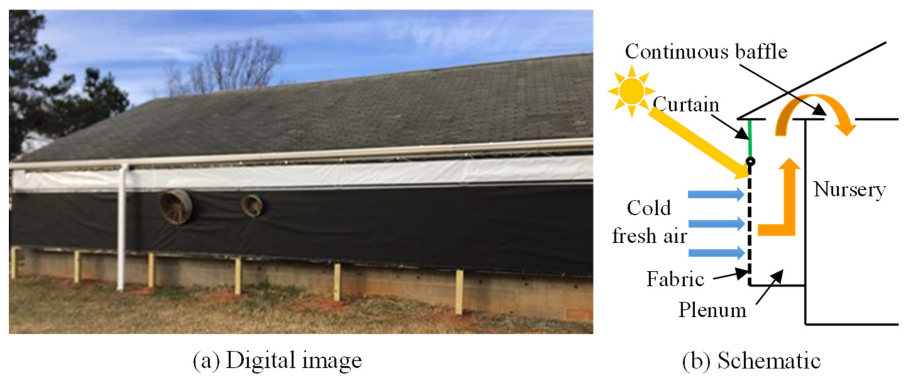
2.1. Nursery Description
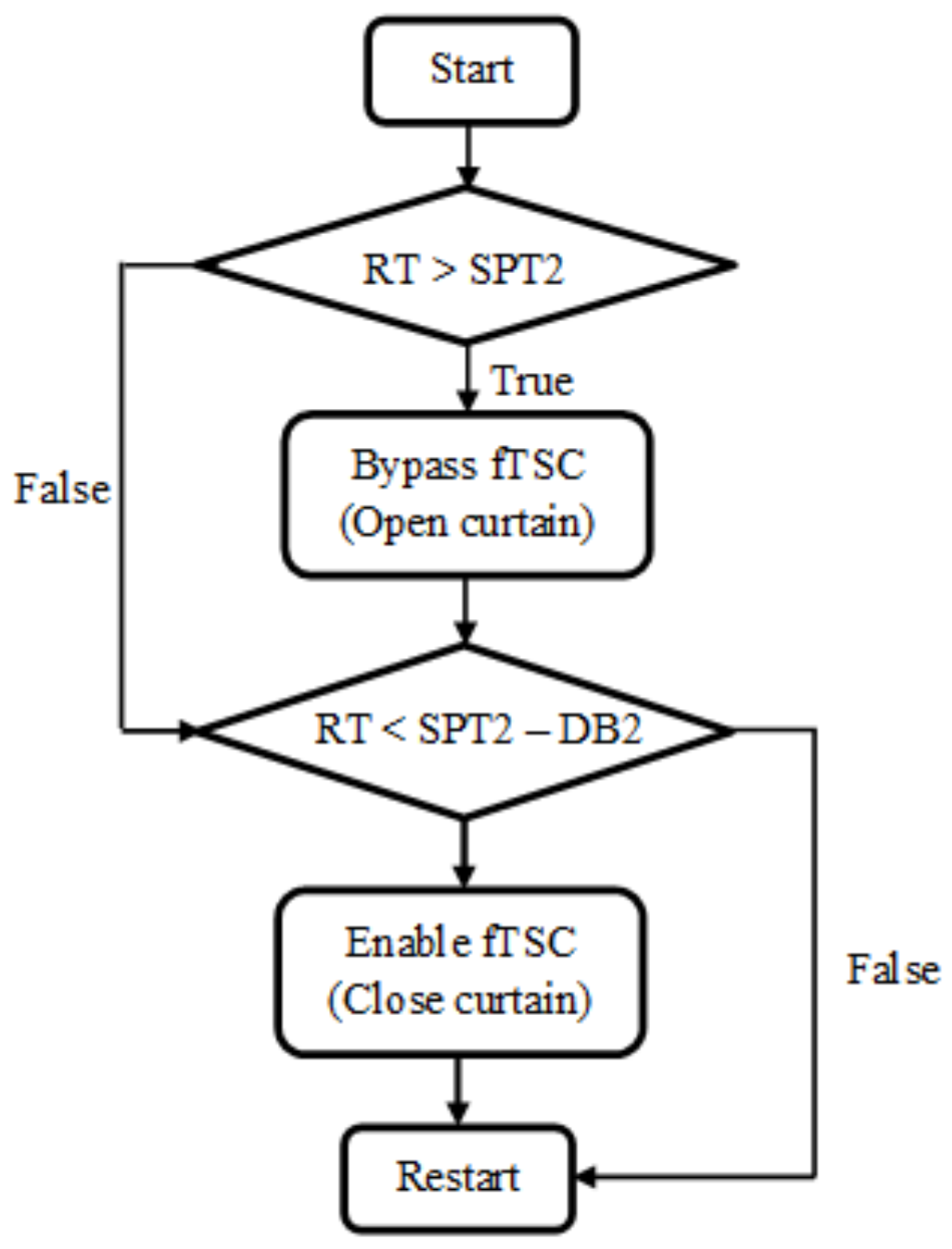
2.2. System Design, Fabrication, and Control
2.3. System Instrumentation and Analyses
2.4. Pig Placement and Management
3. Results and Discussion
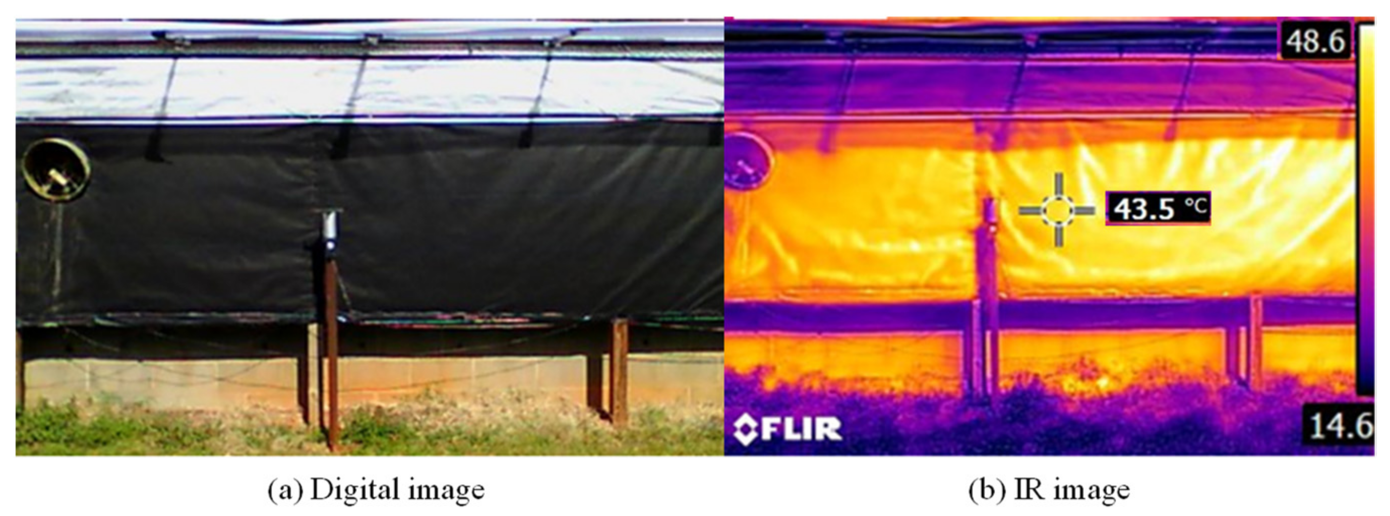
3.1. Performance of fTSC
3.2. Environmental Conditions
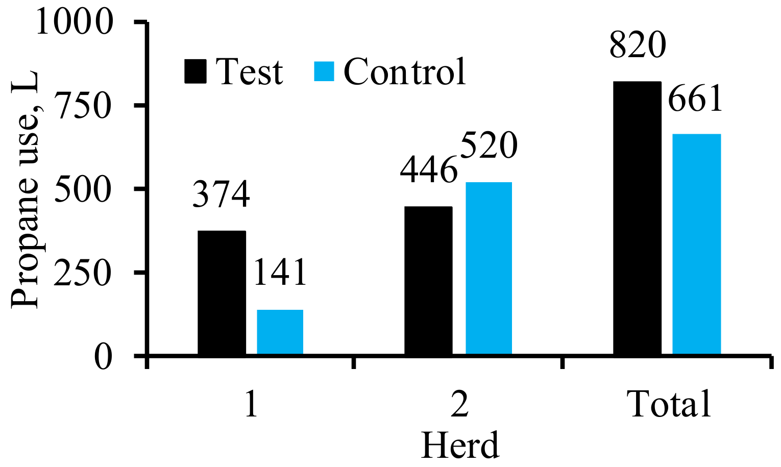
3.3. Propane Use
3.4. Pig Performance
3.5. Scale-Up Considerations
- The fTSC must face preferably, south (or southwest or southeast) in the Northern hemisphere for greater I receipt during winter. Vertical deployment will allow greater I receipt in winter and reduce rainwater ingress than inclined deployment.
- Since heat losses increase with decreasing Vs, operating the fTSC at a higher vs. (perhaps, >0.04 m/s) [10] could improve performance and reduce cost.
- Controlling the fTSC with the barn environmental controller will allow the fans, heaters, and fTSC to work seamlessly. Since commercial houses have lower (and more appropriate) heater capacities [4,5] and ventilation rates [11], the integrated fTSC could work for longer durations, and provide more energy savings.
- While heat recovery increases with PCM area, modeling could be used to determine its cost-effectiveness. Modeling could also include two PCMs with different activation temperatures (e.g., [13]) which might be beneficial also with older piglets that require less heating during daytime while still requiring air tempering after sundown.
4. Conclusions
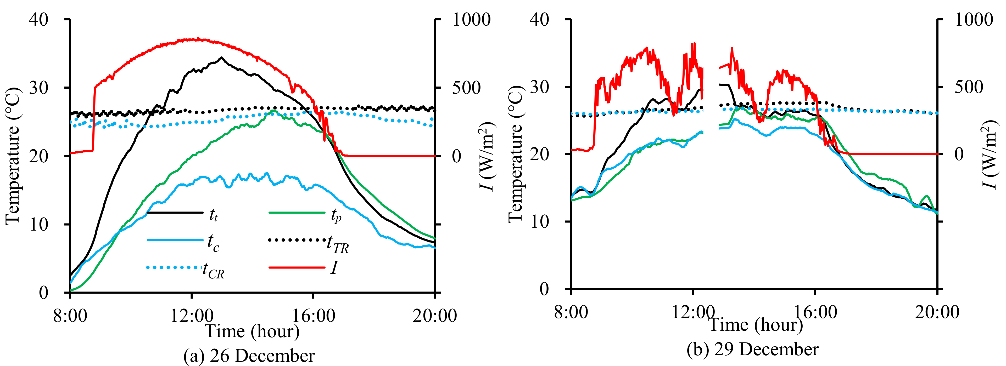
- During 9 h of operation on 26 December 2018, with a mean I of 592 W/m2 the fTSC increased air temperature by a mean of 11.6 °C (maximum of 19.8 °C) with a mean η of 89%. Lower performance on other days might have been due to sub-optimal operating (e.g., intermittent operation) and environmental (e.g., U) conditions.
- For 5 h beginning 4 pm on 26 December 2018, the PCM increased mean air temperature by 3.9 °C, showing that it offered the potential to provide air tempering after sundown.
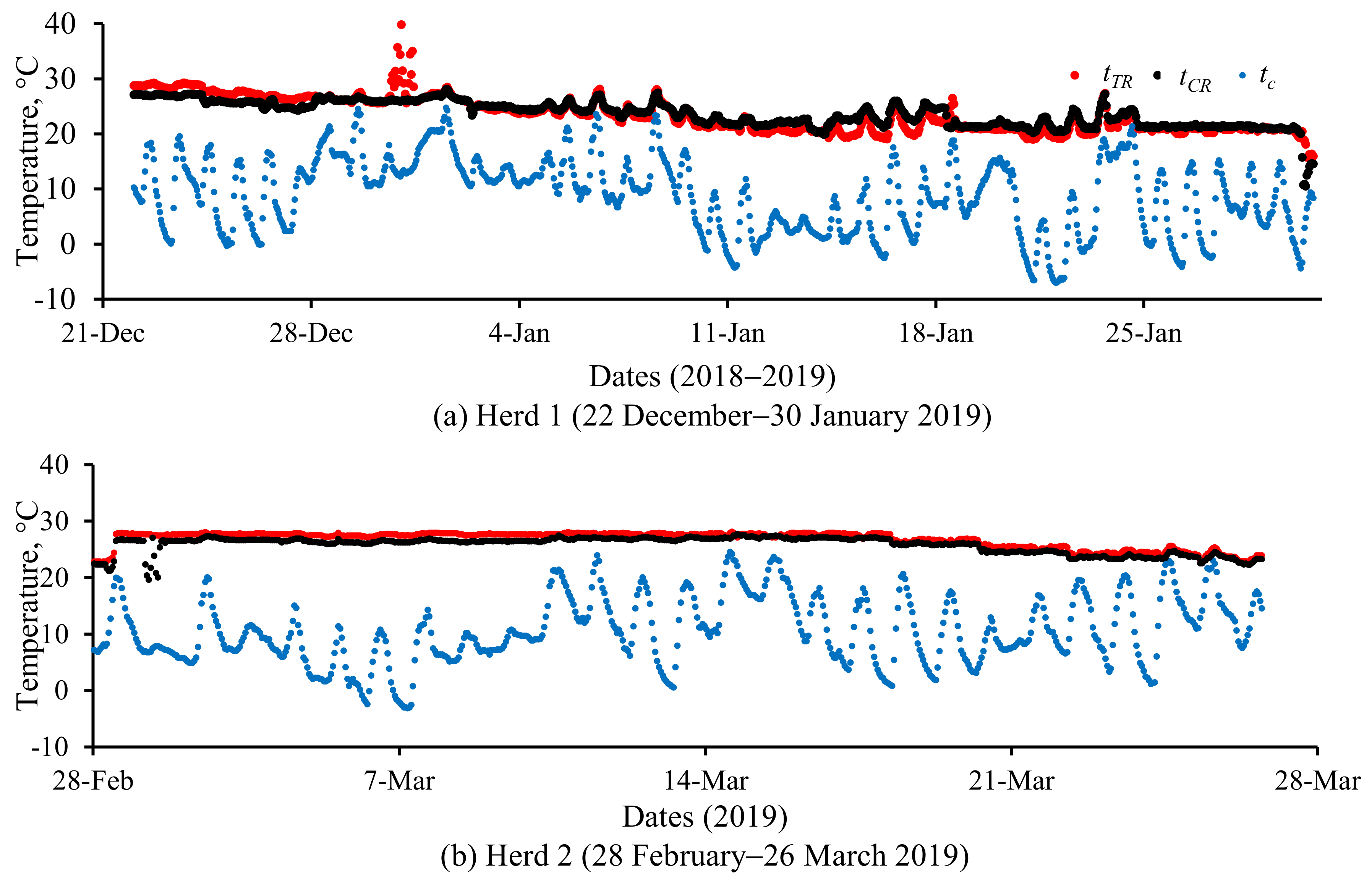
- The Test and Control rooms had the same average air temperatures in Herd 1 but the Test room was slightly warmer in Herd 2. In Herd 1, CO2 concentration was slightly lower and CO concentration slightly higher in the Test room.
- Despite substantial heating of the fresh air, the fTSC did not reduce propane use, probably due to its reduced operation (mainly, breakdowns) and because environmental and fTSC controllers did not work seamlessly.
- Pig performance was unaffected by the treatment.
Author Contributions
Funding
Data Availability Statement
Acknowledgments
Conflicts of Interest
Animal Care and Use
References
- American Society of Heating, Refrigerating and Air-Conditioning Engineers (ASHRAE). Combustion and fuels. In ASHRAE Handbook–Fundamentals; ASHRAE: Atlanta, GA, USA, 2005; Chapter 18. [Google Scholar]
- Kalogirou, S. Solar thermal collectors and applications. Prog. Energy Combust. Sci. 2004, 30, 231–295. [Google Scholar] [CrossRef]
- Kutscher, C.F. Transpired solar collector systems: A major advance in solar heating. In Energy Business Technology Sourcebook, Proceedings of the 19th World Energy Engineering Congress, Atlanta, GA, USA, 6–8 November 1996; NREL Report (No. 24373); National Renewable Energy Laboratory: Golden, CO, USA, 1997; pp. 481–489. [Google Scholar]
- Shah, S.; Marshall, T.; Matthis, S. Transpired solar wall for tempering air in a swine nursery in a humid subtropical climate. Appl. Eng. Agric. 2016, 32, 115–123. [Google Scholar] [CrossRef]
- Love, C.D.; Shah, S.B.; Grimes, J.L.; Willits, D.W. Transpired solar collector duct for tempering air in North Carolina turkey brooder barn and swine nursery. Sol. Energy 2014, 102, 308–317. [Google Scholar] [CrossRef]
- Cordeau, S.; Barrington, S. Performance of unglazed solar ventilation air pre-heaters for broiler barns. Sol. Energy 2011, 85, 1418–1429. [Google Scholar] [CrossRef]
- Bansal, N.; Uhlemann, R. Development and testing of low cost solar energy collectors for heating air. Sol. Energy 1984, 33, 197–208. [Google Scholar] [CrossRef]
- Gawlik, K.M.; Kutscher, C.F. A Numerical and experimental investigation of low-conductivity unglazed, transpired solar air heaters. Sol. Energy 2002, 47–55. [Google Scholar] [CrossRef]
- Poole, M.R.; Shah, S.B.; Grimes, J.L.; Boyette, M.D.; Stikeleather, L.F. Evaluation of a novel, low-cost plastic solar air heater for turkey brooding. Energy Sustain. Dev. 2018, 45, 1–10. [Google Scholar] [CrossRef]
- Poole, M.R.; Shah, S.B.; Boyette, M.D.; Grimes, J.L.; Stikeleather, L.F. Evaluation of landscape fabric as a solar air heater. Renew. Energy 2018, 127, 998–1003. [Google Scholar] [CrossRef]
- Yu, L. Comprehensive Evaluation of a Landscape Fabric Based Transpired Solar Collector in a Pig Nursery. Master’s Thesis, NC State University, Raleigh, NC, USA, 2019. [Google Scholar]
- Liang, Y.; Janorschke, M.; Hayes, C.E. Low-Cost Solar Collectors to Pre-heat Ventilation Air in Broiler Buildings. In Proceedings of the 2021 ASABE Annual International Virtual Meeting, Virtual, 12–16 July 2021; American Society of Agricultural and Biological Engineers (ASABE): St. Joseph, MI, USA, 2021; p. 1. [Google Scholar]
- Poole, M.R.; Shah, S.B.; Boyette, M.D.; Stikeleather, L.F.; Cleveland, T. Performance of a coupled transpired solar collec-tor—phase change material-based thermal energy storage system. Energy Build. 2018, 161, 72–79. [Google Scholar] [CrossRef]
- MidWest Plan Service. MWPS-32 Mechanical Ventilating Systems for Livestock Housing, 1st ed.; Iowa State University: Ames, IA, USA, 1990. [Google Scholar]
- Kutscher, C.F. Heat Exchange Effectiveness and Pressure Drop for Air Flow Through Perforated Plates with and without Crosswind. J. Heat Transf. 1994, 116, 391–399. [Google Scholar] [CrossRef]
- Kaisen Online Calculator. Available online: https://keisan.casio.com/exec/system/1224682277 (accessed on 29 July 2021).
- Kutscher, C.F.; Christensen, C.B.; Barker, G.M. Unglazed Transpired Solar Collectors: Heat Loss Theory. J. Sol. Energy Eng. 1993, 115, 182–188. [Google Scholar] [CrossRef]
- Leon, M.A.; Kumar, S. Mathematical modeling and thermal performance analysis of unglazed transpired solar collectors. Sol. Energy 2007, 81, 62–75. [Google Scholar] [CrossRef]
- Alternative Fuels Data Center (AFDC). Fuel Properties Comparison. Available online: http://www.afdc.energy.gov/fuels/fuel_comparison_chart.pdf (accessed on 29 July 2021).


| Parameters | Fan Setting | |||||
|---|---|---|---|---|---|---|
| 50% | 60% | 70% | 80% | 90% | 100% | |
| Fan speed (rpm) 1 | 907 | 1046 | 1300 | 1376 | 1455 | 1626 |
| Vol. airflow rate (Q, m3/s) 2 | 0.337 | 0.363 | 0.434 | 0.472 | 0.529 | 0.566 |
| Suction velocity (Vs, m/s) 3 | 0.027 | 0.029 | 0.034 | 0.037 | 0.042 | 0.045 |
| Mass airflow rate (kg/s) 4 | 0.399 | 0.430 | 0.514 | 0.559 | 0.626 | 0.670 |
| Period | Pig Age & Dates | tc (°C) | I (W/m2) | Vs (m/s) | Δt (°C) | Δtp (°C) | η (%) | fTSC Operation (%) |
|---|---|---|---|---|---|---|---|---|
| 1 | Day 17–24 1 22–29 December 2018 | 15.5 | 431 | 0.027 | 5.5 | −4.6 | 89 | 98 |
| 2 | Day 3–16 2–15 March 2019 | 14.1 | 258 | 0.027 | 2.6 | −1.0 | 45 | 51 |
| Date & Time | Duration of fTSC Operation (h) | tc (°C) | I (W/m2) | Δt (°C) | Δtp (°C) | η (%) | |
|---|---|---|---|---|---|---|---|
| 26 December | 9.0 | Mean | 13.4 | 592 | 11.6 | −6.9 | 89 |
| Max. 1 | 19.3 | 864 | 19.8 | 0.9 | |||
| 29 December | 8.5 | Mean | 21.2 | 455 | 3.1 | −3.7 | 20 |
| Max. 1 | 26.2 | 822 | 8.2 | 2.3 |
| Date & TIME | Duration of fTSC Operation (h) | tc (°C) | U (m/s) | I (W/m2) | Vs (m/s) | Δt (°C) | Δtp (°C) | η (%) | |
|---|---|---|---|---|---|---|---|---|---|
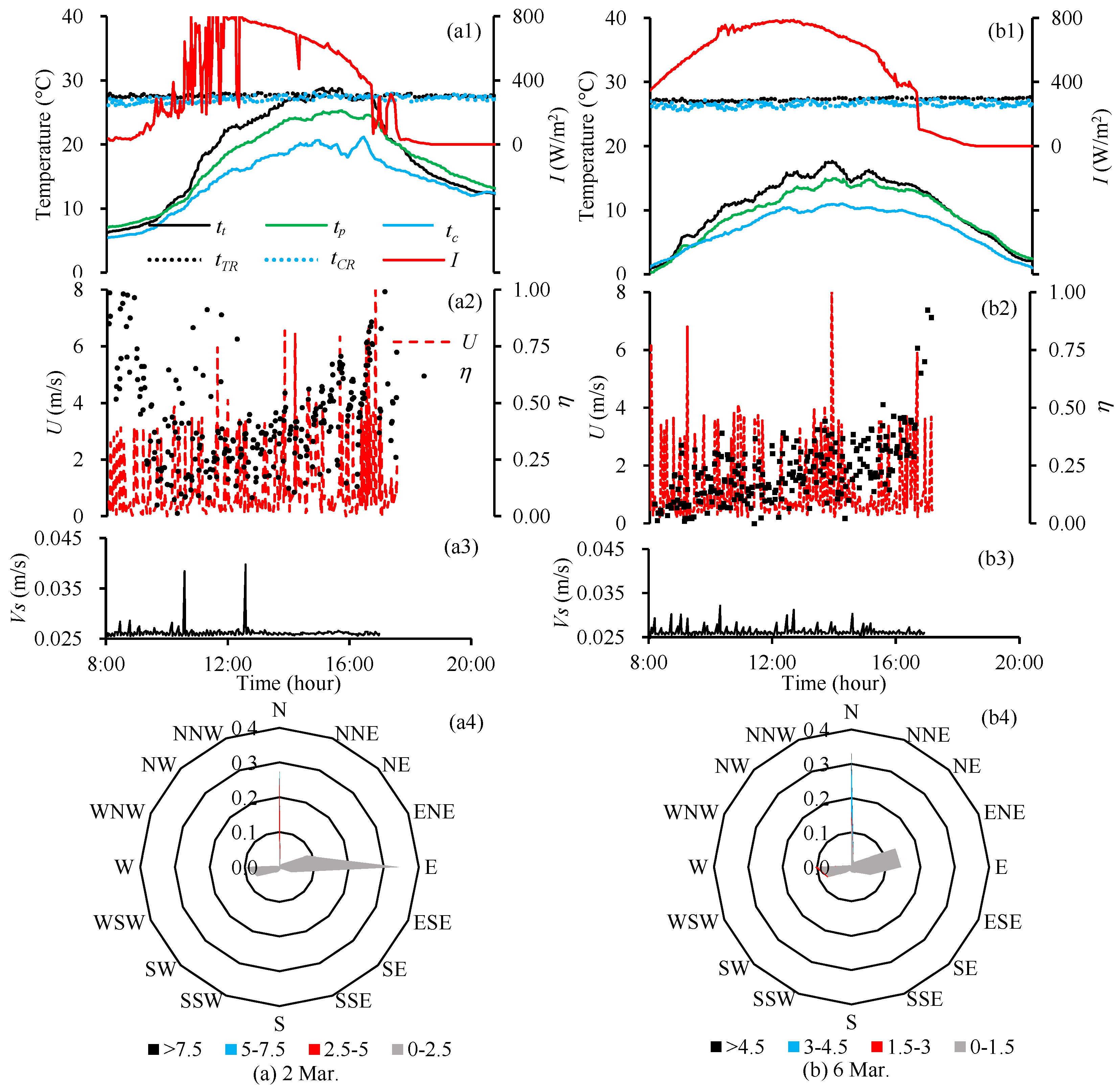
| 2 March | 5.8 | Mean | 15.1 | 1.1 | 450 | 0.027 | 5.6 | −2.1 | 52 |
| Max. 1 | 22.9 | 9.9 | 907 | 0.040 | 12.5 | 2.0 | |||
| 6 March | 5.1 | Mean | 8.0 | 1.2 | 596 | 0.027 | 3.9 | −1.5 | 25 |
| Max. 1 | 12.3 | 8.2 | 788 | 0.032 | 9.9 | 1.7 |
| Herd (Dates) | Temperature (°C) 1 | CO2 (ppm) 2 | CO (ppm) 3 | |||
|---|---|---|---|---|---|---|
| Test | Control | Test | Control | Test | Control | |
| 1 (6 December 2018–30 January 2019) | 23.4 4 | 23.4 4 | 1371 5 | 1441 5 | 1.7 | 1.2 |
| 2 (28 February–4 April 2019) | 26.8 6 | 25.9 6 | Not measured | |||
| Treatment | ADMG 1 (kg/d) | FCR 2 (kg-Feed/kg-Live Mass) | Mortality (%) | |||
|---|---|---|---|---|---|---|
| Herd 1 | Herd 2 | Herd 1 | Herd 2 | Herd 1 | Herd 2 | |
| Test | 0.54 ± 0.08 | 0.36 ± 0.08 | 1.36 | 1.49 | 0.8 | 4.2 |
| Control | 0.55 ± 0.09 | 0.39 ± 0.08 | 1.39 | 1.41 | 0 | 0 |
| p-value 3 | 0.33 | 0.04 | Not analyzed due to lack of replicates | |||
Publisher’s Note: MDPI stays neutral with regard to jurisdictional claims in published maps and institutional affiliations. |
© 2021 by the authors. Licensee MDPI, Basel, Switzerland. This article is an open access article distributed under the terms and conditions of the Creative Commons Attribution (CC BY) license (https://creativecommons.org/licenses/by/4.0/).
Share and Cite
Yu, L.; Shah, S.B.; Knauer, M.T.; Boyette, M.D.; Stikeleather, L.F. Comprehensive Evaluation of a Landscape Fabric Based Solar Air Heater in a Pig Nursery. Energies 2021, 14, 7258. https://doi.org/10.3390/en14217258
Yu L, Shah SB, Knauer MT, Boyette MD, Stikeleather LF. Comprehensive Evaluation of a Landscape Fabric Based Solar Air Heater in a Pig Nursery. Energies. 2021; 14(21):7258. https://doi.org/10.3390/en14217258
Chicago/Turabian StyleYu, Li, Sanjay B. Shah, Mark T. Knauer, Michael D. Boyette, and Larry F. Stikeleather. 2021. "Comprehensive Evaluation of a Landscape Fabric Based Solar Air Heater in a Pig Nursery" Energies 14, no. 21: 7258. https://doi.org/10.3390/en14217258
APA StyleYu, L., Shah, S. B., Knauer, M. T., Boyette, M. D., & Stikeleather, L. F. (2021). Comprehensive Evaluation of a Landscape Fabric Based Solar Air Heater in a Pig Nursery. Energies, 14(21), 7258. https://doi.org/10.3390/en14217258