State-Space Approach for SPMSM Sensorless Passive Algorithm Tuning

Abstract

Sensorless algorithms for Permanent Magnet Synchronous Motors (PMSM) have achieved increasing interest in the technical literature over the last few years. They can be divided into active methods and passive methods: the first inject high-frequency signals exploiting rotor anisotropy, whereas the second are based on observers. Recently, a sensorless control based on a rotor flux observer has been presented in the technical literature, which gives very accurate results in terms of rotor position estimation and robustness. In this paper, the aforementioned observer is considered and a procedure for choosing stabilizing gains of the observer is proposed. The contribution of the paper is three-fold: the mathematical modelling of the rotor flux observer, the methodology for the definition of the observer gains, and the presentation of the experimental results.

1. Introduction

Permanent Magnet Synchronous Motors (PMSMs) are today widely used in industrial applications since they can offer many advantages such as high-power density, high reliability, and efficiency. The field-oriented control (FOC) is one of the most used techniques in order to obtain a good dynamic response [1]; position information is therefore a must-have data for FOC of PMSMs. The main drawbacks arising from the use of position sensors such as resolvers and encoders are the great noise vulnerability and the increasing cost and sizing of the drive, especially for low-power drives [2]. Consequently, many sensorless algorithms for PMSMs have been studied and proposed over the last few years [2,3,4,5,6,7,8,9,10,11,12,13,14,15,16,17,18,19,20,21,22] in order to control the motor without any position sensor, offering significant advantages in terms of reduction of costs, increase of reliability, and removal of wires [3,4]. Sensorless control strategies can be mainly divided into two types: the active methods, using high-frequency signal injection to obtain the information of the rotor position, and the passive methods, consisting of model-based observers, which extract the rotor position by estimating the back electromotive force (back-EMF) or the rotor flux. Since the active methods work well in the low-speed region, while the passive methods guarantee a good performance in the mid to high-speed region, a combination of the two techniques is often used.

Regarding the active methods, some of the possible solutions are the anisotropy-based techniques proposed in [5], and the high-frequency algorithms in [6,7], whereas, among the passive methods, many sensorless control strategies have been proposed, such as the direct back-EMF disturbance observers analysed in [8,9,10,11]. As the back-EMF is proportional to the rotor speed, the efficiency provided by these methods deteriorates at low speeds. For this reason, other common strategies are the Kalman filter-based observers proposed in [4,12], the linkage flux-based observer in [13], and the sliding mode-based observers studied in [14,15,16,17,18,19,20].

The preponderance of the observers proposed in the literature over the past few years work properly under the condition that all electrical motor parameters are exactly known and constant, but these parameters are usually time-varying and uncertain, hence, the design of a robust observer against parameters variation is currently a topic of interest. In [21], Ortega et al. propose a new non-linear flux observer, which is then tested experimentally in [22], and gives very accurate results in terms of rotor position estimation and robustness. A similar observer is introduced by Bobstov et al. [23], and is improved by Choi et al. in [24] by adding a feedback loop to surmount the effect of the permanent-magnet flux linkage constant uncertainty. This robust adaptive observer is tested in different experimental conditions [25].

None of the papers in which this observer is presented show a methodology for the tuning of the two observer gains. Hence, in this paper, the authors are interested in the problem of the design of the two gains of the observer proposed in [24] for a Surface Permanent Magnet Synchronous Motor (SPMSM). Thanks to the linearization of the system and the stability analysis, a satisfactory result is achieved and validated through experimental results. The contents are organized as follows. Section 2 presents the observer and its mathematical modelling, while simulation results are reported in Section 3. Section 4 contains the linearization of the system and the stability analysis which lead to the optimal gains definition. The experimental results are shown in Section 5. Finally, conclusions are drawn in Section 6.

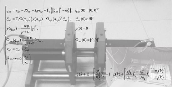
2. RFO Algorithm and Mathematical Modelling

As mentioned in the Introduction, the rotor flux observer (RFO) presented in [23,24] is considered in this paper. Hence, the theoretic description of this algorithm is carried out more deeply in the following. Firstly, the observer proposed in [23] is introduced, and secondly, the feedback loop developed in [24] in order to avoid DC disturbances is explained.

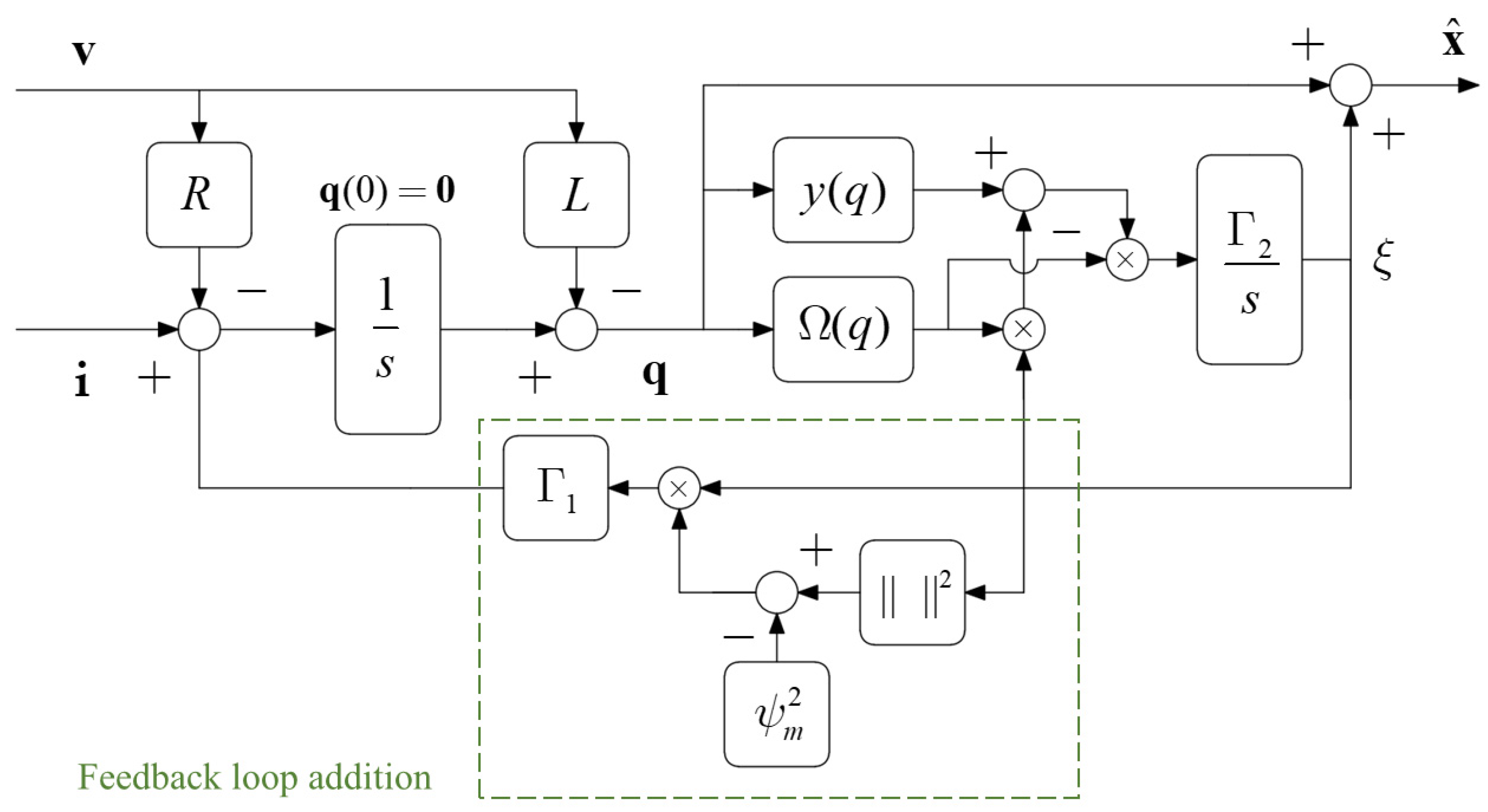
2.1. Observer without the Feedback Loop to Avoid DC Disturbances

If one considers the model of a SPMSM in the stationary $\alpha -\beta$ frame, the stator flux derivative (${\dot{\lambda }}_{\alpha \beta }={[{\dot{\lambda }}_{\alpha },\hspace{0.17em}{\dot{\lambda }}_{\beta }]}^T$) can be defined as in Equation (1) and the stator flux (${\lambda }_{\alpha \beta }={[{\lambda }_{\alpha },\hspace{0.17em}{\lambda }_{\beta }]}^T$) as in Equation (2), being ${\phi }_m$ the Permanent Magnet flux linkage constant and $C_{\alpha \beta }(\theta )={[\cos \theta ,\hspace{0.17em}\sin \theta ]}^T$, while $\theta \in \mathbb{S}:=[0,2\pi ]$ is the rotor flux angle.

$${\dot{\lambda }}_{\alpha \beta }=v_{\alpha \beta }-R{i}_{\alpha \beta }$$

(1)

$${\lambda }_{\alpha \beta }=L{i}_{\alpha \beta }+{\phi }_m{C}_{\alpha \beta }(\theta )$$

(2)

$$\dot{\theta }=\omega$$

(3)

The rotor flux ($x_{\alpha \beta }={[x_{\alpha },\hspace{0.17em}{x}_{\beta }]}^T$) of a SPMSM can be given by Equation (4). If one differentiates both sides of Equation (4), one obtains Equation (5), where J is given by Equation (6) and $p\equiv \frac{d}{dt}$ represents the differential operator.

$$x_{\alpha \beta }\equiv {\lambda }_{\alpha \beta }-L{i}_{\alpha \beta }={\phi }_m{C}_{\alpha \beta }(\theta )$$

(4)

$${\dot{x}}_{\alpha \beta }=v_{\alpha \beta }-R{i}_{\alpha \beta }-Lp{i}_{\alpha \beta }=-{\phi }_m\omega J{C}_{\alpha \beta }(\theta )$$

(5)

$$J=\left[\begin{array}{cc}0& 1\\ -1& 0\end{array}\right]$$

(6)

Since the sensorless algorithm aims to estimate the rotor position, one can calculate such a quantity taking into account Equation (7).

$$\widehat{\theta }={\tan }^{-1}\left(\frac{{\widehat{x}}_{\beta }}{{\widehat{x}}_{\alpha }}\right)$$

(7)

In [23] an observer with zero initial value is proposed; the state observer $q_{\alpha \beta }$ is defined as in Equation (8).

$${\dot{q}}_{\alpha \beta }(t)=v_{\alpha \beta }-R{i}_{\alpha \beta }-Lp{i}_{\alpha \beta },\hspace{0.17em}\hspace{0.17em}\hspace{0.17em}\hspace{0.17em}\hspace{0.17em}q(0)={[0,\hspace{0.17em}\hspace{0.17em}0]}^T$$

(8)

Please note that $q_{\alpha \beta }$ and $x_{\alpha \beta }$ have the same dynamics, but different initial conditions. If one defines ${\xi }_{\alpha \beta }={\lambda }_{\alpha \beta }(0)-L{i}_{\alpha \beta }(0)$, it follows Equation (9).

$$x_{\alpha \beta }(t)=q_{\alpha \beta }(t)+{\xi }_{\alpha \beta }$$

(9)

Since ${\Vert q_{\alpha \beta }+{\xi }_{\alpha \beta }\Vert }^2={\Vert x_{\alpha \beta }\Vert }^2$ and ${\Vert x_{\alpha \beta }\Vert }^2={\phi }_m^2$, one can obtain from Equation (9) the relation in Equation (10)

$$-{\Vert q_{\alpha \beta }\Vert }^2=2q_{\alpha \beta }^T\hspace{0.17em}{\xi }_{\alpha \beta }+{\Vert {\xi }_{\alpha \beta }\Vert }^2-{\phi }_m^2$$

(10)

In order to obtain a linear regression form, it is necessary to differentiate Equation (10). However, a pure derivative is always associated with noise amplification in real applications, therefore a high-pass filter $\frac{\alpha p}{p+\alpha }$ can be applied to both sides of Equation (10). Indeed, $\frac{\alpha p}{p+\alpha }=p\cdot \frac{\alpha }{p+\alpha }$, i.e., it is a derivative for low-frequencies but with a low-pass filter form. Applying the high-pass filter to Equation (10) one obtains Equation (11), where $y(q_{\alpha \beta })$ and ${\mathrm{\Omega }}_{\alpha \beta }(q_{\alpha \beta })$ are defined in Equations (12) and (13).

$$y(q_{\alpha \beta })={\mathrm{\Omega }}_{\alpha \beta }{(q_{\alpha \beta })}^T{\xi }_{\alpha \beta }+\epsilon (t)$$

(11)

$$y(q_{\alpha \beta })=\frac{-\alpha p}{p+\alpha }\left({\Vert q_{\alpha \beta }\Vert }^2\right)$$

(12)

$${\mathrm{\Omega }}_{\alpha \beta }(q_{\alpha \beta })=\frac{2\alpha p}{p+\alpha }(q_{\alpha \beta })$$

(13)

Since ${\Vert \xi \Vert }^2-{\phi }_m^2$ is a constant, one obtains Equation (14) for some C > 0.

$$\epsilon (t)=\frac{p\alpha }{p+\alpha }\left({\Vert \xi \Vert }^2-{\phi }_m^2\right)=\alpha C{e}^{-\alpha t}$$

(14)

Equation (11) represents a linear regression equation with an unknown parameter $\xi$. Indeed, it is a product of a known vector ${\mathrm{\Omega }}_{\alpha \beta }(q_{\alpha \beta })$, by ${\xi }_{\alpha \beta }$. Therefore, a parameter estimator can be derived using the descent gradient method, obtaining Equations (15) and (16), where $\mathrm{\Gamma }$ is a gain matrix. The derived sensorless control scheme is shown in Figure 1.

$${\dot{\xi }}_{\alpha \beta }=\mathrm{\Gamma }{\mathrm{\Omega }}_{\alpha \beta }(q_{\alpha \beta })(y(q_{\alpha \beta })-{\mathrm{\Omega }}_{\alpha \beta }{(q_{\alpha \beta })}^T{\xi }_{\alpha \beta }),\hspace{0.17em}\hspace{0.17em}\hspace{0.17em}\hspace{0.17em}\hspace{0.17em}{\xi }_{\alpha \beta }(0)\in {\Re }^2$$

(15)

$$\hspace{0.17em}{\xi }_{\alpha \beta }(0)={\phi }_m\left[\cos ({\theta }_0);\hspace{0.17em}\hspace{0.17em}\sin ({\theta }_0)\right]$$

(16)

2.2. Feedback Addition to Avoid DC Disturbances

A non-linear feedback loop was added in [24] in order to avoid the problems connected to DC disturbances, as highlighted in blue in Figure 2.

Adding the feedback containing ${\mathrm{\Gamma }}_1$ gain, the observer defined by Equation (17) is obtained.

$$\{\begin{array}{l}{\dot{q}}_{\alpha \beta }=v_{\alpha \beta }-R{i}_{\alpha \beta }-Lp{i}_{\alpha \beta }+{\mathrm{\Gamma }}_1\left({\Vert {\xi }_{\alpha \beta }\Vert }^2-{\phi }_m^2\right),\hspace{0.17em}\hspace{0.17em}\hspace{0.17em}{q}_{\alpha \beta }(0)={[0,\hspace{0.17em}\hspace{0.17em}0]}^T\\ {\dot{\xi }}_{\alpha \beta }={\mathrm{\Gamma }}_2\mathrm{\Omega }(q_{\alpha \beta })\left(y(q_{\alpha \beta })-{\mathrm{\Omega }}_{\alpha \beta }{(q_{\alpha \beta })}^T{\xi }_{\alpha \beta }\right),\hspace{0.17em}\hspace{0.17em}\hspace{0.17em}\hspace{0.17em}\hspace{0.17em}\hspace{0.17em}\hspace{0.17em}\hspace{0.17em}\hspace{0.17em}\hspace{0.17em}{\xi }_{\alpha \beta }(0)\in {\Re }^2\\ y(q_{\alpha \beta })=\frac{-\alpha p}{p+\alpha }{\Vert q\Vert }^2,\hspace{0.17em}\hspace{0.17em}\hspace{0.17em}\hspace{0.17em}\hspace{0.17em}\hspace{0.17em}\hspace{0.17em}\hspace{0.17em}\hspace{0.17em}\hspace{0.17em}\hspace{0.17em}\hspace{0.17em}\hspace{0.17em}\hspace{0.17em}\hspace{0.17em}\hspace{0.17em}\hspace{0.17em}\hspace{0.17em}\hspace{0.17em}\hspace{0.17em}\hspace{0.17em}\hspace{0.17em}\hspace{0.17em}\hspace{0.17em}\hspace{0.17em}\hspace{0.17em}\hspace{0.17em}\hspace{0.17em}\hspace{0.17em}\hspace{0.17em}\hspace{0.17em}\hspace{0.17em}\hspace{0.17em}\hspace{0.17em}\hspace{0.17em}\hspace{0.17em}\hspace{0.17em}\hspace{0.17em}\hspace{0.17em}\hspace{0.17em}\hspace{0.17em}y(0)=0\\ {\mathrm{\Omega }}_{\alpha \beta }(q_{\alpha \beta })=\frac{\alpha p}{p+\alpha }2q_{\alpha \beta },\hspace{0.17em}\hspace{0.17em}\hspace{0.17em}\hspace{0.17em}\hspace{0.17em}\hspace{0.17em}\hspace{0.17em}\hspace{0.17em}\hspace{0.17em}\hspace{0.17em}\hspace{0.17em}\hspace{0.17em}\hspace{0.17em}\hspace{0.17em}\hspace{0.17em}\hspace{0.17em}\hspace{0.17em}\hspace{0.17em}\hspace{0.17em}\hspace{0.17em}\hspace{0.17em}\hspace{0.17em}\hspace{0.17em}\hspace{0.17em}\hspace{0.17em}\hspace{0.17em}\hspace{0.17em}\hspace{0.17em}\hspace{0.17em}\hspace{0.17em}\hspace{0.17em}\hspace{0.17em}\hspace{0.17em}\hspace{0.17em}\hspace{0.17em}\hspace{0.17em}\hspace{0.17em}\hspace{0.17em}{\mathrm{\Omega }}_{\alpha \beta }(0)={[0,\hspace{0.17em}0]}^T\\ x_{\alpha \beta }=q_{\alpha \beta }+{\xi }_{\alpha \beta }\\ \widehat{\theta }=atan2\left(\frac{x_{\beta }}{x_{\alpha }}\right)\end{array}$$

(17)

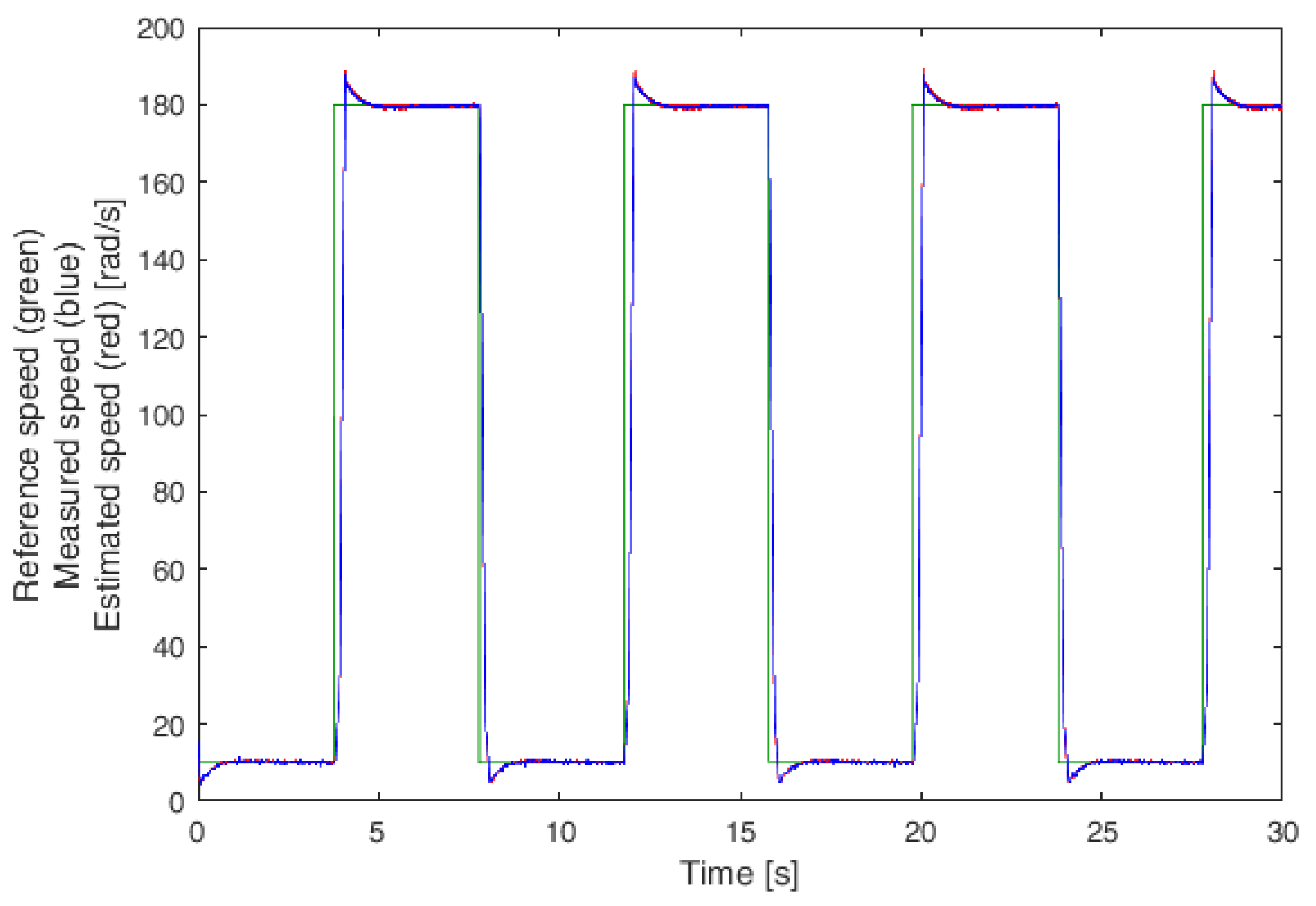
3. Simulation Results

In this section, some simulation results are reported in order to better understand the working principle of the RFO considered in this study. Both simulations for the observer proposed in [23] and for the one with the addition of the feedback loop to eliminate DC disturbances [24] are shown below, respectively, as similarly shown in Section 2 for the theoretical description.

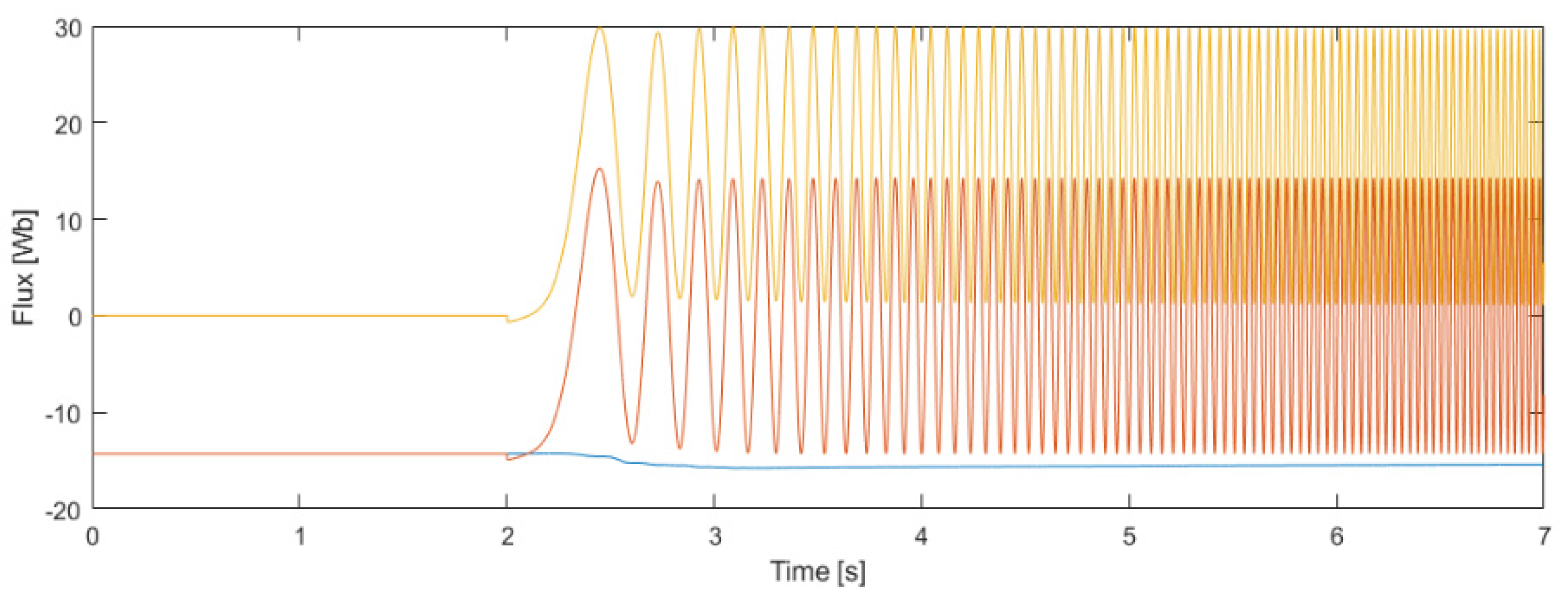
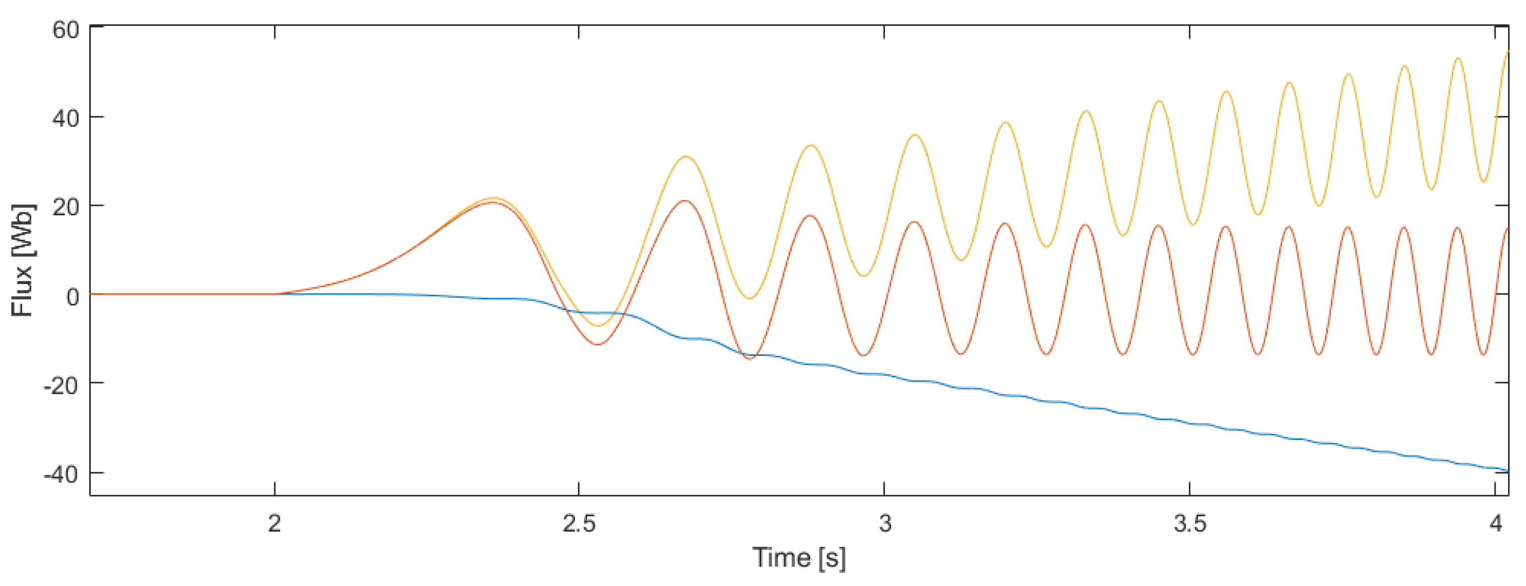
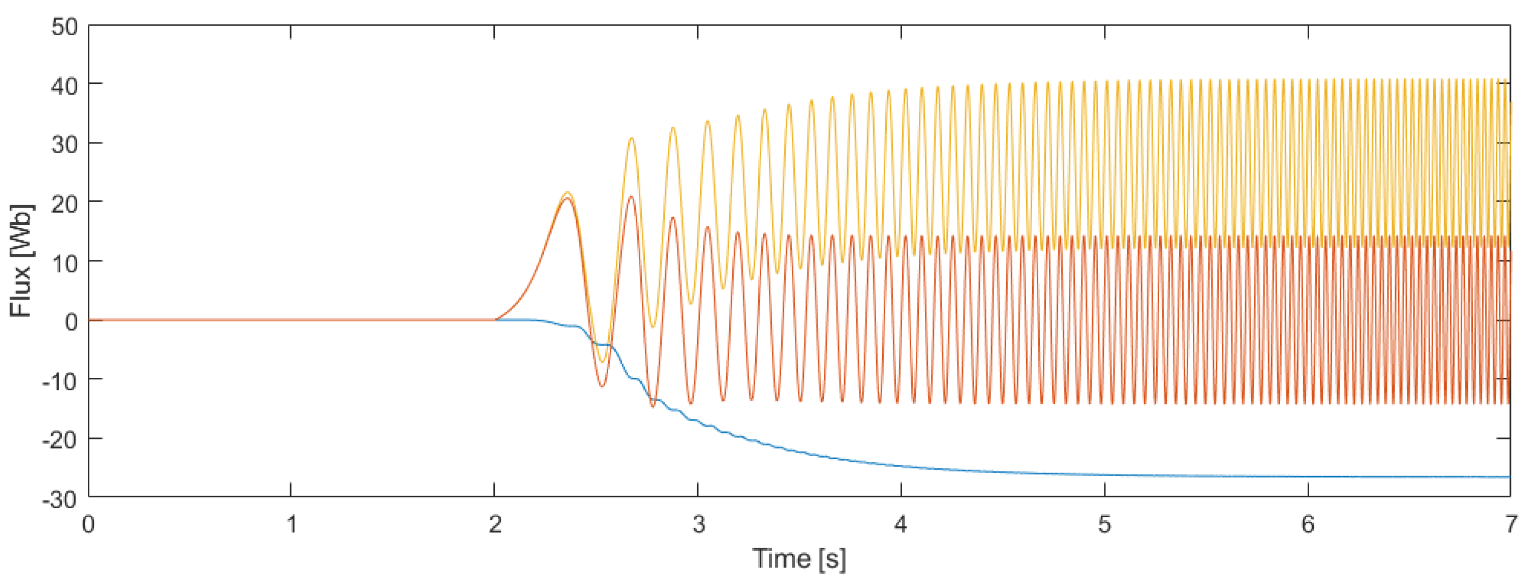
3.1. Observer without the Feedback Loop to Avoid DC Disturbances

The RFO proposed in [23] has been built in MATLAB/Simulink environment, and some simulation results are shown in the following. Since $q_{\alpha \beta }$ is initialized at zero, the two vector components are affected by a bias error. This bias is related to the real initial rotor angle. For simplicity, one can consider the case in which ${\theta }_0=-90°$ and ${\xi }_{\alpha \beta }$ is correctly initialized, i.e., as in Equation (18). In this condition, $q_{\alpha \beta }$ is given by Equation (19) and $x_{\alpha \beta }$ is given by Equation (20). Indeed, the bias of $q_{\beta }$ is corrected by ${\xi }_{\beta }$, as shown in Figure 3, where simulation results in this particular condition are shown and $q_{\beta }$, ${\xi }_{\beta }$, and $x_{\beta }$ are plotted. In this case, the bias is corrected from the beginning because ${\xi }_{\alpha \beta }$ is initialized correctly, otherwise, the estimator loop provides the correct bias correction. Please note that the bias of $q_{\beta }$ is inherent in the observer definition; indeed both Equations (18) and (19), and simulation results of Figure 3 are obtained in ideal conditions.

$$\{\begin{array}{l}{\xi }_{\alpha }={\phi }_m\cos ({\theta }_0)=0\\ {\xi }_{\beta }={\phi }_m\sin ({\theta }_0)=-{\phi }_m\end{array}$$

(18)

$$\{\begin{array}{l}{q}_{\alpha }={\displaystyle \int v_{\alpha }-R{i}_{\alpha }=}\hspace{0.17em}{\phi }_m\cos (\theta )\\ q_{\beta }={\displaystyle \int v_{\beta }-R{i}_{\beta }={\phi }_m+{\phi }_m\sin (\theta )}\end{array}$$

(19)

$$\{\begin{array}{l}{x}_{\alpha }={\phi }_m\cos (\theta )\\ x_{\beta }={\phi }_m\sin (\theta )\end{array}$$

(20)

The observer proposed in [23] is straightforward and easy to implement. However, it is sensible to DC disturbances, due to the presence of a pure integrator. As an example, one can consider the previous case, with a negative DC error on $i_{\alpha }$ measure. In this case, $q_{\alpha }$ is given by Equation (21) and therefore it diverges. The same simulation results of Figure 3 are shown for this case in Figure 4.

Please note that the observer diverges even if ${\xi }_{\alpha \beta }$ is correctly initialized, as it can be shown more easily in the simulation plot with time enlargement in Figure 5.

$$q_{\alpha }={\displaystyle \int v_{\alpha }-R(i_{\alpha }-i_{\alpha DC})=}\hspace{0.17em}{\phi }_m\cos (\theta )+{\displaystyle \int R{i}_{\alpha DC}}$$

(21)

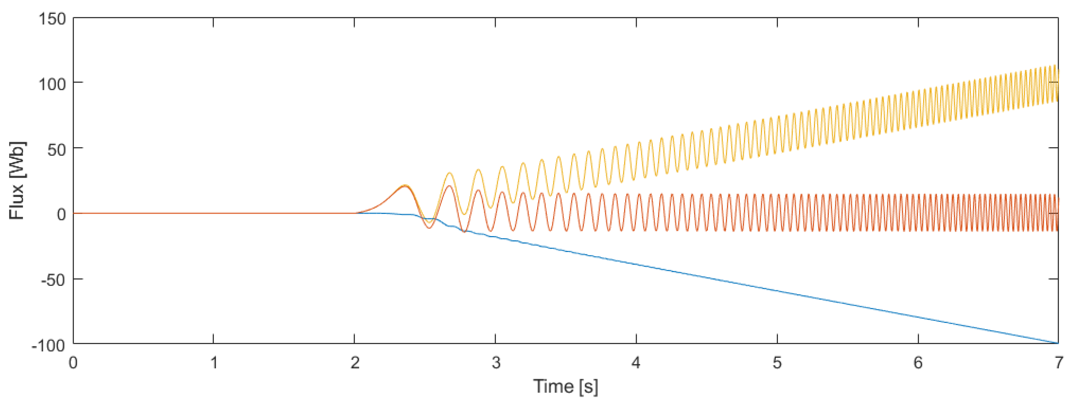
3.2. Observer with the Addition of the Feedback Loop to Avoid DC Disturbances

The simulation with $i_{\alpha }$ DC disturbance was carried out with the sensorless algorithm defined in Equation (17) and the results are shown in Figure 6. One can note that with the addition of the feedback containing ${\mathrm{\Gamma }}_1$ gain, has a null average value and $q_{\alpha }$ does not diverge anymore; hence, a more robust result is achieved.

4. Definition of ${\mathrm{\Gamma }}_2$ Gain

From the results shown in the previous section, one can note that the feedback loop containing ${\mathrm{\Gamma }}_1$ gain aims at increasing the robustness of the system avoiding $q_{\alpha \beta }$ divergence. Since it does not directly affect the estimator inner loop (containing ${\mathrm{\Gamma }}_2$ gain), its influence on the estimator dynamic is limited. On the contrary, the estimator loop containing ${\mathrm{\Gamma }}_2$ gain is the core of the RFO observer, therefore an appropriate tuning of such a parameter is fundamental to achieve a good drive dynamic response.

Even if this sensorless technique was proposed in [23,24], none of these papers show a methodology for ${\mathrm{\Gamma }}_2$ tuning, which is proposed in this paper. If one considers the loop shown in Figure 7, the inputs of the loop are $u_1=y(q_{\alpha \beta })$ and $u_2={\mathrm{\Omega }}_{\alpha \beta }(q_{\alpha \beta })$.

${\dot{\xi }}_{\alpha \beta }$ is defined in Equation (22). Please note that for notation simplicity, the αβ subscripts are omitted in the following Equations and complex number notation is exploited. Since the function $f_1$ is non-linear, a linearization process should be carried out, as shown in Equation (23). Moreover, since motor drives are discrete systems, Equation (23) is linearized as in Equation (24), obtaining the linearized and discretized Equation of the loop in (27) after the algebraic simplifications of Equations (25) and (26). Evaluating the eigenvalues as in Equation (28), one obtains Equation (29), where Tc is the sampling time.

$$\dot{\xi }=f_1={\mathrm{\Gamma }}_2{u}_2(u_1-u_2\xi )$$

(22)

$$\dot{\xi }=\left[\frac{\partial f_1}{\partial \widehat{\xi }}\right]\left[\xi \right]+\left[\frac{\partial f_1}{\partial u_1}\frac{\partial f_1}{\partial u_2}\right]\left[\begin{array}{c}{u}_1\\ u_2\end{array}\right]$$

(23)

$$\frac{\xi (k+1)-\xi (k)}{T_C}=\frac{\partial f_1}{\partial \widehat{\xi }}\xi (k)+\left[\frac{\partial f_1}{\partial u_1}\hspace{0.17em}\hspace{0.17em}\hspace{0.17em}\frac{\partial f_1}{\partial u_2}\right]\left[\begin{array}{c}{u}_1(k)\\ u_2(k)\end{array}\right]$$

(24)

$$\xi (k+1)=\frac{\partial f_1}{\partial \widehat{\xi }}\xi (k)T_C+\xi (k)+\left[\frac{\partial f_1}{\partial u_1}\hspace{0.17em}\hspace{0.17em}\hspace{0.17em}\hspace{0.17em}\frac{\partial f_1}{\partial u_2}\right]\left[\begin{array}{c}{u}_1(k)\\ u_2(k)\end{array}\right]T_C$$

(25)

$$\xi (k+1)=\left[\frac{\partial f_1}{\partial \widehat{\xi }}{T}_C+1\right]\xi (k)+\left[\frac{\partial f_1}{\partial u_1}{T}_C\hspace{0.17em}\hspace{0.17em}\hspace{0.17em}\hspace{0.17em}\frac{\partial f_1}{\partial u_2}{T}_C\right]\left[\begin{array}{c}{u}_1(k)\\ u_2(k)\end{array}\right]$$

(26)

$$\xi (k+1)=A\hspace{0.17em}\xi (k)+B\left[\begin{array}{c}{u}_1(k)\\ u_2(k)\end{array}\right],\hspace{0.17em}\hspace{0.17em}\hspace{0.17em}\hspace{0.17em}\hspace{0.17em}\hspace{0.17em}\hspace{0.17em}\hspace{0.17em}\hspace{0.17em}\hspace{0.17em}A=-{\mathrm{\Gamma }}_2{u}_2^2{T}_C+1$$

(27)

$$A-\lambda =-{\mathrm{\Gamma }}_2{u}_2^2{T}_C+1-\lambda$$

(28)

$$\lambda =-{\mathrm{\Gamma }}_2{u}_2^2{T}_C+1$$

(29)

If one approximates the output of the observer as a sinusoidal function, as in Equation (30), and neglects the low-pass filter of ${\mathrm{\Omega }}_{\alpha \beta }(q_{\alpha \beta })$ function, Equation (31) is derived. Neglecting the stator resistance and the stator inductance, i.e., considering $\Vert \psi \omega \Vert =\Vert v\Vert$, where $v$ represents the peak phase voltage value (e.g., 310 V for a 380 V motor), since the $\alpha -\beta$ domain is used, one can define the eigenvalues as in Equation (32).

$$q_{\alpha \beta }={\left[{\phi }_m\cos (\omega t),\hspace{0.17em}\hspace{0.17em}\hspace{0.17em}{\phi }_m\sin (\omega t)\right]}^T$$

(30)

$$u_2=2pq={[-2\phi \omega \sin (\omega t),\hspace{0.17em}\hspace{0.17em}2\phi \omega \cos (\omega t)\hspace{0.17em}]}^T$$

(31)

$$\lambda =-4{\mathrm{\Gamma }}_2{v}^2{T}_C+1$$

(32)

Since, according to the classical control theory, a discrete system is stable if the eigenvalues are inside the circle with a centre in the axis origin and a unitary radius, it follows that the loop of Figure 7 is stable if the condition in Equation (33) is verified. Imposing null eigenvalue, the gain ${\mathrm{\Gamma }}_2$ can be defined as in Equation (34).

$$-2<-4{\mathrm{\Gamma }}_2{v}^2{T}_C<0$$

(33)

$$\lambda =0\hspace{0.17em}\hspace{0.17em}\hspace{0.17em}\hspace{0.17em}\to \hspace{0.17em}{\mathrm{\Gamma }}_2=\frac{1}{4v^2{T}_C}$$

(34)

In Equation (31) the low pass filter is neglected, i.e., the condition in Equation (35) is imposed. Indeed, the high-pass filter can be seen as a combination of a low-pass filter with the derivative operation, as specified in Equation (36). It is interesting to note that when the frequency of the stator voltage is higher than the cut-off frequency of the filter, the eigenvalue is defined as in Equation (37). Since this condition in Equation (38) is verified, it follows that, from a stability point of view, neglecting the low-pass filter is a conservative hypothesis.

$$u_2=\frac{p\alpha }{p+\alpha }2q\cong 2pq$$

(35)

$$\frac{s\alpha }{s+\alpha }=s\frac{\alpha }{s+\alpha }$$

(36)

$$\omega \gg \alpha \to \lambda =-4{\mathrm{\Gamma }}_2{(\psi \alpha )}^2{T}_C+1$$

(37)

$$4{\mathrm{\Gamma }}_2{(\psi \alpha )}^2{T}_C<4{\mathrm{\Gamma }}_2{v}^2{T}_C$$

(38)

As mentioned above, the gain ${\mathrm{\Gamma }}_1$ is not critical and its design does not affect significantly the stability of the system compared to ${\mathrm{\Gamma }}_2$; hence, in the following, the relation ${\mathrm{\Gamma }}_1={\mathrm{\Gamma }}_2$ has been imposed.

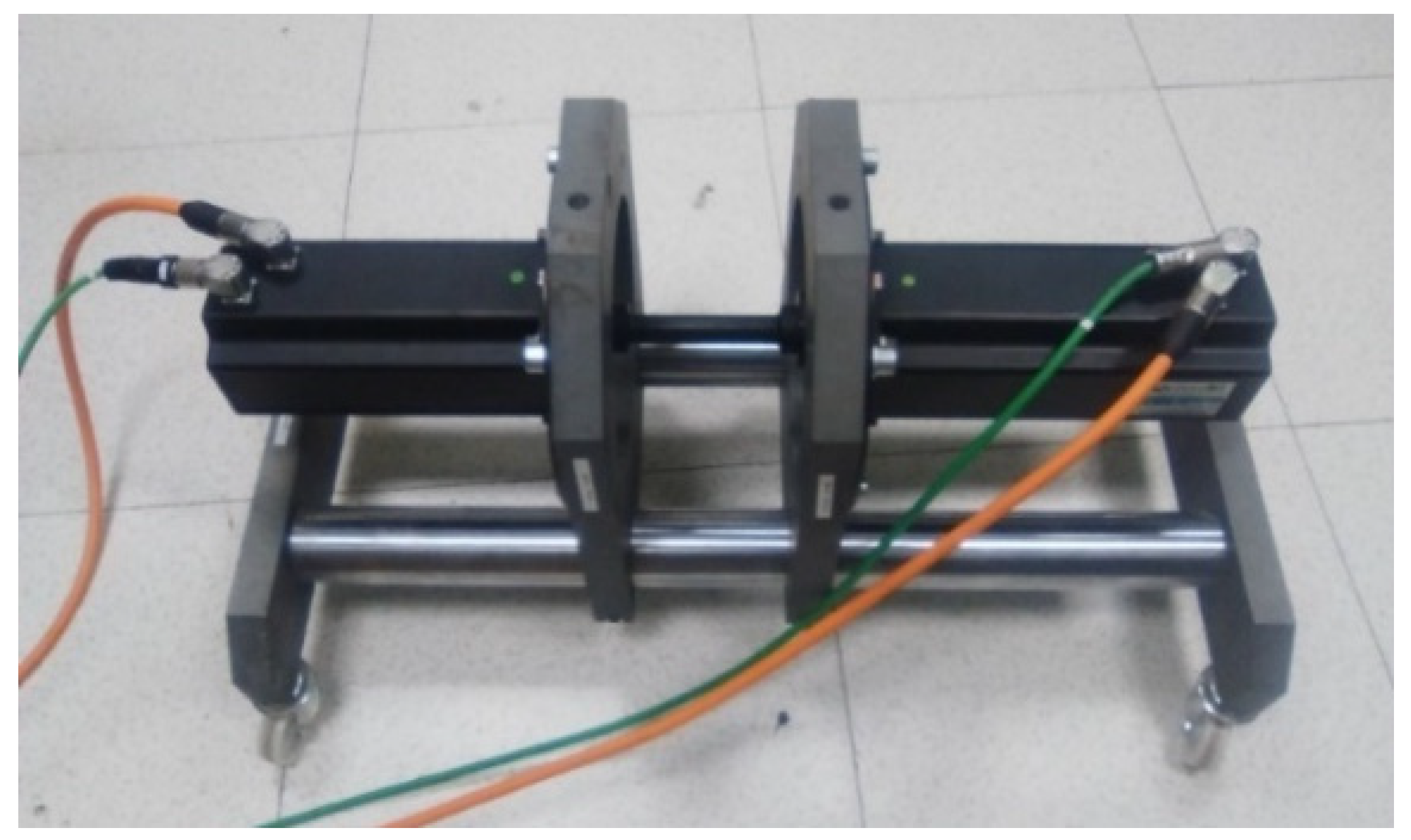
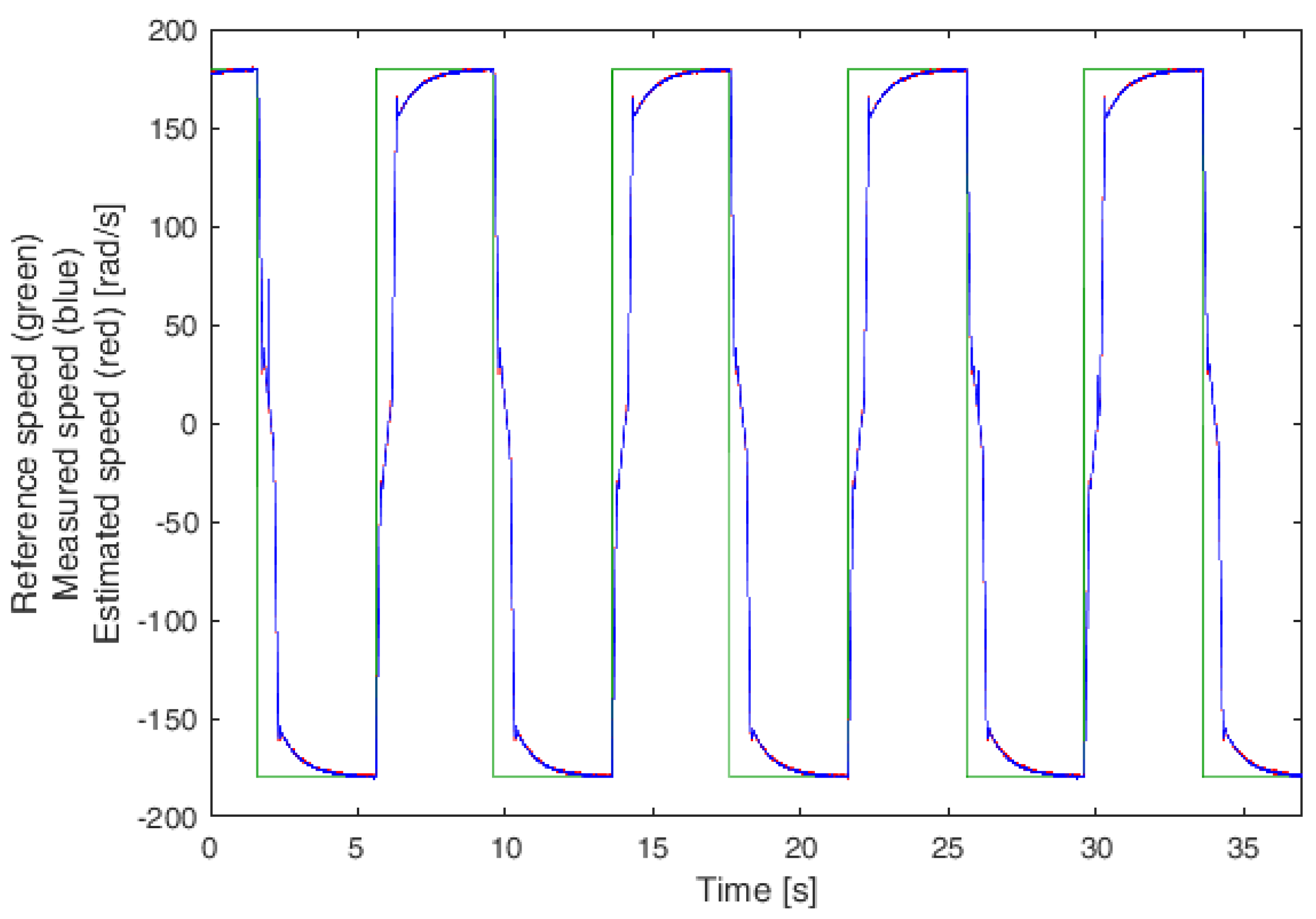
5. Experimental Results

Some experimental tests have been carried out in order to evaluate the performance of the gain definition analysis presented in the previous section. The observer was implemented in DSpace Microlab Box (dSPACE GmbH, Paderborn, Germany) control platform and the test bench is reported in Figure 8.

Table 1. Motor data.

Parameter	Value
Rated output power	5600 W
Rated phase voltage RMS	380 V
Pole pairs	4
Rated speed	2000 rpm
Rated torque	27 Nm
Rated current	11.9 A
$\mathrm{Flux} \mathrm{constant} {\phi }_m$	0.335 Wb
Stator resistance Rs	0.68 Ω
Stator inductance Ls	5.0 mH
Sampling time Tc	200 μs

and

Table 2. Observer gains.

Parameter	Value
$\mathrm{Gain} {\mathrm{\Gamma }}_1$	0.013
$\mathrm{Gain} {\mathrm{\Gamma }}_2$	0.013

show, respectively, the motor parameters and the observer gains, which are selected with the methodology presented in the previous section.

The DSpace system outputs were sent to a PWM inverter (rated current: 300 A, DC link voltage: 550 V) connected to the SPMSM. Both the sampling frequency and the PWM switching frequency were set to 5 kHz. The inverter nonlinearities were non-compensated and the deadtime was 4 µs. A 27 Nm SPMSM was coupled with the test motor and used to provide the load torque when needed. The two tests performed are listed as follows:

Test 1: a speed reference variation between 180 rad/s and −180 rad/s with linear load torque (rated torque at rated speed);

Test 2: a speed reference variation between 180 rad/s and 5 rad/s with no-load.

Figure 9 shows measured and estimated speed during a reference variation between 180 rad/s and −180 rad/s (Test 1), while in Figure 10, the results of Test 2 are reported. It can be noted from Figure 9 and Figure 10 that the speed reference is correctly followed both with and without the starting load torque.

6. Conclusions

A robust sensorless algorithm for a SPMSM is considered. It is based on the rotor flux observer proposed in [21,22,23], and it was improved with a non-linear feedback loop in [24]. The mathematical modelling of the observer is presented in Section 2, while Section 3 contains some simulation results. None of the papers in which this observer is analysed show a methodology for an optimal design of the two observer gains.

This paper discusses the architecture of the observer and the effects of the gains ${\mathrm{\Gamma }}_1$ and ${\mathrm{\Gamma }}_2$ on the system. In particular, since the feedback loop containing ${\mathrm{\Gamma }}_1$ gain aims at increasing the robustness of the system with DC disturbances, but it does not directly affect the estimator inner loop (containing ${\mathrm{\Gamma }}_2$ gain), its influence on the observer dynamic is limited. Hence, the contribution of ${\mathrm{\Gamma }}_1$ can be neglected, while the procedure used to define an optimal solution for ${\mathrm{\Gamma }}_2$ is proposed in Section 4. The linearization of the non-linear discrete system and the stability analysis are achieved and validated through the experimental results presented in Section 5. The two tests reported in Figure 9 and Figure 10 show that the speed reference is correctly followed both with and without the starting load torque, with the gains selected with the methodology presented.

References

1. Lara, J.; Chandra, A. Performance Investigation of Two Novel HSFSI Demodulation Algorithms for Encoderless FOC of PMSMs Intended for EV Propulsion. IEEE Trans. Ind. Electron. 2017, 65, 1074–1083. [Google Scholar] [CrossRef]
2. Pando-Acedo, J.; Romero-Cadaval, E.; Milanes-Montero, M.I.; Barrero-Gonzalez, F. Improvements on a Sensorless Scheme for a Surface-Mounted Permanent Magnet Synchronous Motor Using Very Low Voltage Injection. Energies 2020, 13, 2732. [Google Scholar] [CrossRef]
3. Dwivedi, P.K.; Seth, A.K.; Singh, M. Sensorless Speed Control of PMSM Motor for Wide Speed Range. In Proceedings of the 2021 1st International Conference on Power Electronics and Energy (ICPEE), Bhubaneswar, India, 2–3 January 2021. [Google Scholar]
4. Dilys, J.; Stankevič, V.; Łuksza, K. Implementation of Extended Kalman Filter with Optimized Execution Time for Sensorless Control of a PMSM Using ARM Cortex-M3 Microcontroller. Energies 2021, 14, 3491. [Google Scholar] [CrossRef]
5. Ogasawara, S.; Akagi, H. Implementation and Position Control Performance of a Position-Sensorless IPM Motor Drive System Based on Magnetic Saliency. IEEE Trans. Ind. Appl. 1998, 34, 806–812. [Google Scholar] [CrossRef] [Green Version]
6. Liu, J.M.; Zhu, Z.Q. Sensorless Control Strategy by Square-Waveform High-Frequency Pulsating Signal Injection Into Stationary Reference Frame. IEEE J. Emerg. Sel. Top. Power Electron. 2013, 2, 171–180. [Google Scholar] [CrossRef]
7. Tuovinen, T.; Hinkkanen, M. Adaptive Full-Order Observer with High-Frequency Signal Injection for Synchronous Reluctance Motor Drives. IEEE J. Emerg. Sel. Top. Power Electron. 2013, 2, 181–189. [Google Scholar] [CrossRef] [Green Version]
8. Chen, Z.; Tomita, M.; Doki, S.; Okuma, S. An extended electromotive force model for sensorless control of interior permanent-magnet synchronous motors. IEEE Trans. Ind. Electron. 2003, 50, 288–295. [Google Scholar] [CrossRef]
9. Wang, G.; Ding, L.; Li, L.; Xu, J.; Zhang, G.; Zhan, H.; Ni, R.; Xu, D. Enhanced Position Observer Using Second-Order Generalized Integrator for Sensorless Interior Permanent Magnet Synchronous Motor Drives. IEEE Trans. Energy Convers. 2014, 29, 486–495. [Google Scholar]
10. Kim, J.; Jeong, I.; Nam, K.; Yang, J.; Hwang, T. Sensorless Control of PMSM in a High-Speed Region Considering Iron Loss. IEEE Trans. Ind. Electron. 2015, 62, 6151–6159. [Google Scholar] [CrossRef]
11. Rajamani, R. Observers for Lipschitz nonlinear systems. IEEE Trans. Autom. Control. 1998, 43, 397–401. [Google Scholar] [CrossRef]
12. Quang, N.K.; Hieu, N.T.; Ha, Q. FPGA-Based Sensorless PMSM Speed Control Using Reduced-Order Extended Kalman Filters. IEEE Trans. Ind. Electron. 2014, 61, 6574–6582. [Google Scholar] [CrossRef]
13. Gierczynski, M.; Grzesiak, L. Comparative Analysis of the Steady-State Model Including Non-Linear Flux Linkage Surfaces and the Simplified Linearized Model when Applied to a Highly-Saturated Permanent Magnet Synchronous Machine—Evaluation Based on the Example of the BMW i3 Traction Motor. Energies 2021, 14, 2343. [Google Scholar]
14. Yan, Z.; Utkin, V. Sliding mode observers for electric machines—An overview. In Proceedings of the IEEE 2002 28th Annual Conference of the Industrial Electronics Society. IECON 02, Seville, Spain, 5–8 November 2002; pp. 1842–1847. [Google Scholar]
15. Wang, G.; Li, Z.; Zhang, G.; Yu, Y.; Xu, D. Quadrature PLL-Based High-Order Sliding-Mode Observer for IPMSM Sensorless Control With Online MTPA Control Strategy. IEEE Trans. Energy Convers. 2013, 28, 214–224. [Google Scholar] [CrossRef]
16. Hongryel, K.; Jubum, S.; Jangmyung, L. A High-Speed Sliding-Mode Observer for the Sensorless Speed Control of a PMSM. IEEE Trans. Ind. Electron. 2011, 58, 4069–4077. [Google Scholar] [CrossRef]
17. Qiao, Z.; Shi, T.; Wang, Y.; Yan, Y.; Xia, C.; He, X. New Sliding-Mode Observer for Position Sensorless Control of Permanent-Magnet Synchronous Motor. IEEE Trans. Ind. Electron. 2013, 60, 710–719. [Google Scholar] [CrossRef]
18. Liang, D.; Li, J.; Qu, R. Sensorless Control of Permanent Magnet Synchronous Machine Based on Second-Order Sliding-Mode Observer With Online Resistance Estimation. IEEE Trans. Ind. Appl. 2017, 53, 3672–3682. [Google Scholar] [CrossRef]
19. Bao, D.; Wu, H.; Wang, R.; Zhao, F.; Pan, X. Full-Order Sliding Mode Observer Based on Synchronous Frequency Tracking Filter for High-Speed Interior PMSM Sensorless Drives. Energies 2020, 13, 6511. [Google Scholar] [CrossRef]
20. Haus, B.; Mercorelli, P.; Aschemann, H. Gain Adaptation in Sliding Mode Control Using Model Predictive Control and Disturbance Compensation with Application to Actuators. Information 2019, 10, 182. [Google Scholar] [CrossRef] [Green Version]
21. Ortega, R.; Praly, L.; Astolfi, A.; Lee, J.; Nam, K. Estimation of Rotor Position and Speed of Permanent Magnet Synchronous Motors With Guaranteed Stability. IEEE Trans. Control. Syst. Technol. 2010, 19, 601–614. [Google Scholar] [CrossRef]
22. Junggi, L.; Jinseok, H.; Kwanghee, N.; Ortega, R.; Praly, L.; Astolfi, A. Sensorless Control of Surface-Mount Permanent-Magnet Synchronous Motors Based on a Nonlinear Observer. IEEE Trans. Power Electron. 2010, 25, 290–297. [Google Scholar] [CrossRef] [Green Version]
23. Bobtsov, A.A.; Pyrkin, A.A.; Ortega, R.; Vukosavic, S.N.; Stankovic, A.M.; Panteley, E.V. A robust globally convergent position observer for the permanent magnet synchronous motor. Automatica 2015, 61, 47–54. [Google Scholar] [CrossRef]
24. Choi, J.; Nam, K.; Bobtsov, A.; Pyrkin, A.; Ortega, R. Robust Adaptive Sensorless Control for Permanent-Magnet Synchronous Motors. IEEE Trans. Power Electron. 2017, 32, 3989–3997. [Google Scholar] [CrossRef]
25. Marchesoni, M.; Passalacqua, M.; Vaccaro, L.; Calvini, M.; Venturini, M. Performance improvement in a sensorless surface-mounted PMSM drive based on rotor flux observer. Control. Eng. Pract. 2020, 96, 104276. [Google Scholar] [CrossRef]
Figure 1. Observer and parameter estimator proposed in [23].
Energies 14 07180 g001
Figure 2. Observer and parameter estimator proposed in [24].
Energies 14 07180 g002
Figure 3. qβ (yellow), ξβ (blue) and xβ (red) when θ0 = 0, estimator shown in [23], φ m = 14 Wb.
Energies 14 07180 g003
Figure 4. qα (yellow), ξα (blue) and xα (red) when θ0 = 0 and with iα negative DC error, estimator shown in [23], φ m = 14 Wb.
Energies 14 07180 g004
Figure 5. qα (yellow), ξα (blue) and xα (red) when θ0 = 0 and with iα negative DC error, estimator shown in [23], time axis enlargement, φ m = 14 Wb.
Energies 14 07180 g005
Figure 6. qα (yellow), ξα (blue) and xα (red) when θ0 = 0 and with iα negative DC error, estimator shown in [24].
Energies 14 07180 g006
Figure 7. Γ2 loop of estimator proposed in [24].
Energies 14 07180 g007
Figure 8. Test bench.
Energies 14 07180 g008
Figure 9. Reference, measured and estimated speed during Test 1 (speed step from 180 rad/s to −180 rad/s with linear load torque).
Energies 14 07180 g009
Figure 10. Reference, measured and estimated speed during Test 2 (speed step from 180 rad/s to 5 rad/s with no-load).
Energies 14 07180 g010