Abstract
This paper presents a comparison between two design methodologies applied to permanent magnet synchronous machines for hybrid and electric vehicles (HEVs and EVs). Both methodologies are based on 2D finite element models and coupled to a genetic algorithm to optimize complex non-linear geometries such as multi-layer permanent magnet machines. To reduce the computation duration to evaluate Induced Voltage and Iron Losses for a given electrical machine configuration, a new methodology based on geometrical symmetries and magnetic symmetries are used and is detailed. Two electromagnetic models have been developed and used in the design stage. The first model was the stepped rotor position finite element analysis called abc model which considered the spatial harmonics without any approximation of the waveform of flux linkage inside the stator, and the second model was based on a fixed rotor position called dq model, with the approximation that the waveform of flux linkage inside the stator was sinuous. These two methodologies are applied to the design of a synchronous machine for HEVs and EVs applications. Design results and performances are analyzed, and the advantages and drawbacks of each methodology are presented. It was found that the dq model is at least 5 times faster than the abc model with high precision for both the torque and induce voltage evaluation in most cases. However, it is not the case for the iron losses computation. The iron loss model based on dq model is less accurate than the abc model with a relative deviation from the abc model greater than 70% at high control angle. The choice of the electromagnetic model during the optimization process will therefore influence the geometry and the performances of the obtained electrical machine after the optimization.
1. Introduction
Electric vehicles (EVs) appear today as one of the solutions supported by the policies of many countries to reduce pollution and achieve global climate change objectives. The electric vehicle is suitable for urban use. The main obstacles to its deployment are the cost of the vehicle and access to charging. Reducing the cost of electric vehicles involves reducing the cost of powertrain components. The main components of an electric vehicle’s powertrain are the battery, the power converter, and the electric motor. The battery is one of the most important parts of the conversion chain due to its limited on-board energy and high cost (around 30% of the vehicle price). To efficiently use this on-board energy, we would need to optimize the energy efficiency of the other powertrain components. In this article, we are interested in the optimal design of the electrical machine.
The optimization of electrical machines is a multi-objective, multi-physics, high-dimensional, highly non-linear and coupled problem challenging both industries and research communities [1,2,3,4,5,6,7]. An electrical machine dedicated to automotive applications, has to be designed against driving cycles rather than against one single point [8]. Driving cycles are generally composed of more than thousands of operating points. Thus, the optimization of electrical machines based on finite elements calculation is generally time consuming, especially in the case where parameter control of each operating point has to be found during the optimization process. Only some works have been done on optimization of electrical machines by considering the whole operating points. These studies are based on using electromagnetic analytical models for simple geometry and validated by finite element (FE) calculation [2]. In [3], a parametric design method for surface-mounted permanent magnet synchronous machines (SPM) is presented by an electromagnetic design against driving cycle and validated by a magnetic equivalent circuit model of the machine. However, most electrical machines used for automotive applications are synchro-reluctant and highly saturated machines [4]. The saturation of magnetic materials is generally not considered in analytical models. Therefore, they are not suitable for designing these types of machines.
The FE has the advantage to be accurate compared to the analytical models and is applicable to solve non-linear and highly saturated problems and especially complex machine’s geometries but may suffer from high computation time. To reduce the computation time for optimization of electric machines using finite element calculations, the driving cycle is reduced to few equivalent operating points [9,10,11,12]. The energy over the entire driving cycle is evaluated and some equivalent operating points are extracted with appropriate weights to have an equal energy consumption. In [5], a clustering methodology is applied to reduce the NEDC operating points to 12 representative operating points. The energy consumption calculated with the 12 points is 2% lower than the real energy over the torque speed envelope. From these few representative operating points, optimization based on finite elements calculation can be made by considering different electromagnetic models such as the stepped rotor position and the fixed rotor position [6].
In the same way of reducing computation time of FE calculation, some approximate models have been developed such as response surface models (RSM), radial basis functions models (RBF), Kriging model and artificial neural network models [7]. Response surface models (RSM) is the most popular optimization methodology to design an electrical machine for EV/HEV. It is based on semi finite elements approach (FEA) and more adapted to design an electrical machine against driving cycle constraints [8]. This methodology combines fixed rotor position FEA and analytical models based on flux linkage maps extracted from FEA to compute the objectives and constraints. Fixed rotor position FEA is used to create a flux linkage map. The flux linkage maps are used by the analytical models to evaluate the machine performances on the entire torque-speed envelope. The approximate models are more efficient for the design of an electrical machine that has more than 20 operating points. A computationally efficient technique for fast and accurate electrical machine performance evaluations over the entire operating envelope is proposed in [8]. This method used a response surface model based on FEA to generate a polynomial expression for flux linkage and loss. The proposed methods have been validated with experimental measurements on their in-house 35 kW IPM traction motor and from published data on the 2004 Toyota Prius motor.
The methodologies described above are quite promising in the scope of electrical machine design for automotive applications, especially the approximate response surface model (RSM). However, these papers did not discuss the limits of these analytical models used for creating the RSM. The analytical flux linkage models are computed in d-axis and q-axis flux linkages which are based on the first harmonic flux linkage hypothesis. Regarding the high weakening region, especially in the design of high-speed machines, this hypothesis is no longer valid because the wave form of flux linkages is not sinuous. Therefore, the contribution of this paper is twofold. At first, we will propose a fast and accurate multi-objective and multi-physical optimization method for the design of an electrical machine based on finite element evaluation. The electromagnetic models of the proposed methodology use geometrical symmetries and magnetic symmetries to reduce the computation time of the classical stepped rotor position by 3. Secondly, we analyzed and compared the fixed rotor position model used to build SRM to the stepped rotor position model and show the limits of the fixed rotor position model for complex geometry in high weakening region.
2. Multi-Objective and Multi-Physics Optimization Methodology
The global optimization framework is shown in Figure 1. The optimization methodology has been developed on MATLAB® and based on 2D finite element-modeling tool XFEMM® to calculate the electromagnetic performances of the machine [13]. For the choice of optimization algorithms in optimization process, we used the platform PlatEmo [14]. PlatEmo is an open source MATLAB platform for evolutionary multi-objective optimization, which includes more than 50 multi-objective evolutionary algorithms with several used performance indicators.
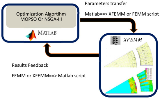
Figure 1.
MATLAB and XFEMM connection for the optimization process.
2.1. Optimization Procedure
An optimization problem for multi-objective with constraints can be defined as:
where and . are respectively the objective functions, constraints, and design parameters.
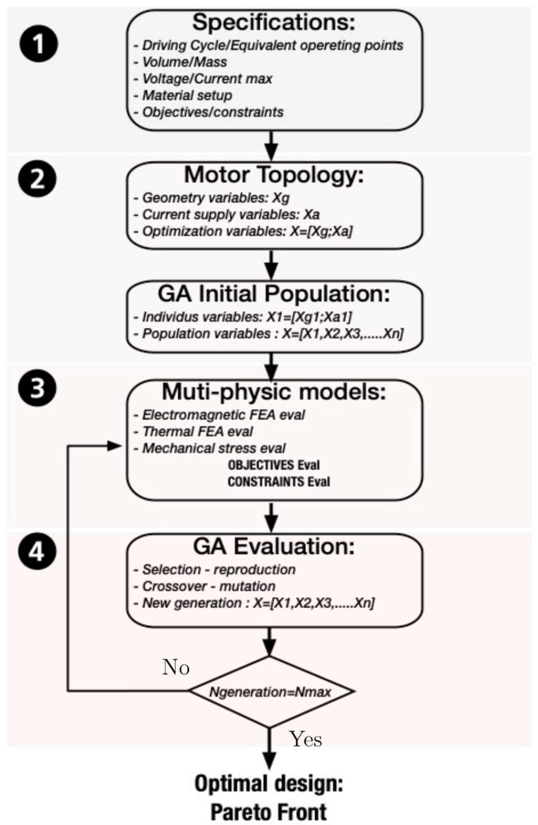
A flow chart of the proposed multi-physics optimization design based on the Genetic Algorithm (NSGA III) is shown in Figure 2. The optimization methodology proposed in this paper is an iterative process based on Genetic Algorithm (GA) [15,16,17] evaluation which consists of four parts:
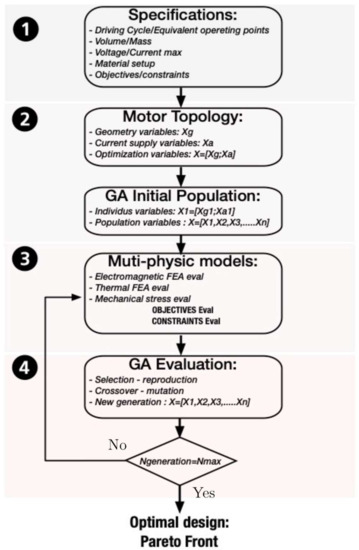
Figure 2.
Optimization Algorithm Flow chart.
Step 1: To design the powertrain system, the specifications of the drive system must be defined such as requiring torque-speed operating points, the rated power, voltage, current, speed range, volume, cost, etc.
Step 2: From the specifications, we chose a specific motor topology and we parametrized its geometry (Figures 4 and 5). For geometrical variables, we had to add the control parameter variables. Two variables for each operating point, the current (Imax) and the torque angle control ψ. The optimization variables combine geometric variables and supply variables. Then, based on the optimization variables defined, we used GA to generate randomly the first generation of the population (by MATLAB® “rand” function) or directly imposed by the user.
Step 3: we computed the multi-physical FEA (electromagnetic, thermal, and mechanical) to evaluate the objective functions and constraints which will be used by GA to optimize the electrical machine.
Step 4: From objective functions and constraints evaluation, the GA performs some operations such as selection, crossovers and mutation to produce the following generations. The GA parameters used by default in PlatEmo are given in [18]: probability of crossover (proC): 1; distribution index of crossover (disC): 20; probability of mutation (proM): 1; distribution index of mutation (disM): 20
The optimization process is terminated when the number of generations reaches a given value.
2.2. Motor Topology
By analyzing the different types of powertrains (EVs/HEVs) already commercialized, we noticed a diversity of electric machine technologies such as permanent magnet synchronous machines (PMs), induction machines and wound field synchronous machines. The most used are PMs due to their high torque and power density. Figure 3 shows the different rotor geometries used in the recent EV and HEV powertrains. These rotor topologies are principally based on V-shaped, double V-shaped, or double layer topologies, etc.

Figure 3.
Rotors of electric machines for the recent hybrid electric vehicles (HEVs) and electric vehicles (EVs).
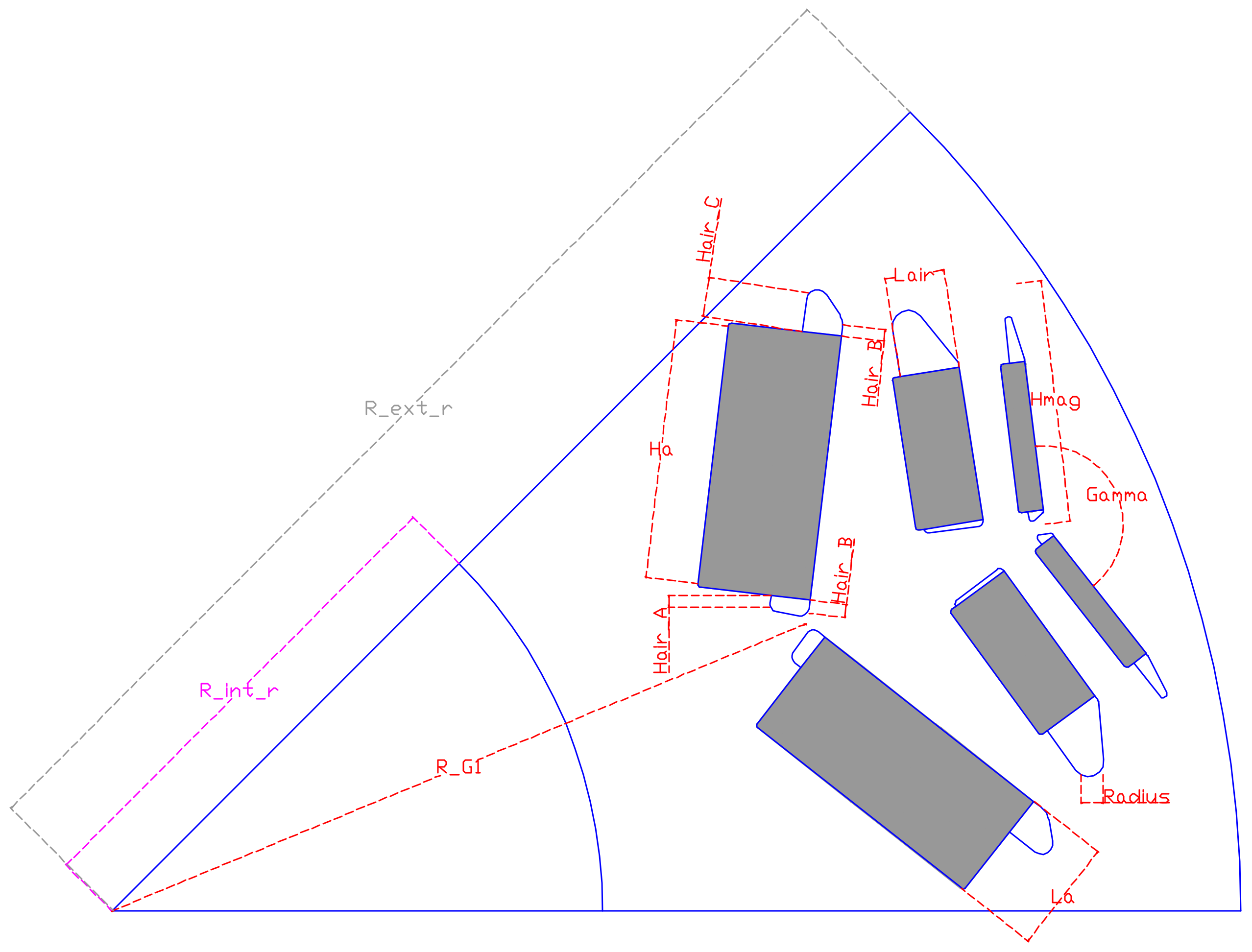
We propose in this paper a multi-layer topology allowing modeling the rotor topologies presented in Figure 3. All the geometry is parameterized, and optimization variables have been shown in Figure 4 and Figure 5 (in red and magenta). We add fillet variable around the corner for each magnet layer to have better evaluation of mechanical stress. The discrete variables such as phase numbers, pole numbers, slots per pole per phase, winding configurations are fixed parameters during the optimization routine and can be modified at the beginning of each optimization process.
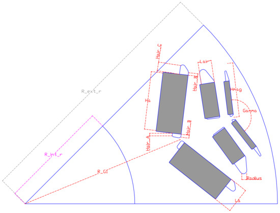
Figure 4.
Rotor geometry parameters.

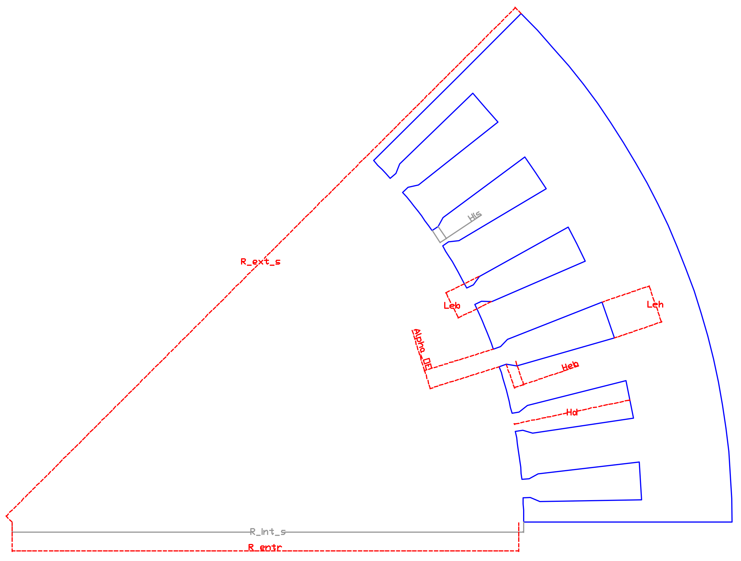
Figure 5.
Stator geometry parameters.
The optimization geometric parameters depend on the number of magnet layers. The description of all geometric optimization parameters is given in Figure 4 and Figure 5 and Table 1. Each magnet layer has 10 variables to well describe its shape, direction, position, the bridge between two magnets of the same layer and air pocket around. To magnet variables, the interior rotor radius variable is added to well describes the rotor. The total variables of the rotor are then , where is the number of magnet layers.

Table 1.
Optimization parameters description.
The stator has variables allowing to model, the active length of laminations, the stator external diameter, the opening slot, stator tooth length, the bottom stator slot width, the top stator slot width, and the isthmus height. The optimization variables are dimensionless and normalized with respect to its maximum available length, to have comparable variables on a unit basis.
The total optimization variables are:
- Geometric variables:
- Supply variables:
is the number of electric machine operating points.
2.3. Electromagnetic Models Stepped Rotor Position (abc Model) vs. Fixed Rotor Position (dq Model)
The electromagnetic performances are evaluated by FE calculations to have the most generic design tool for modeling complex geometries. Indeed, the FE modeling allows an easy adaptation of the models developed for the evaltion of the performances of the machine in the case we have to change the geometry of the machine. The main disadvantage of FE modeling is the high computation time. To overcome the computation time issue, we developed two electromagnetic models (stepped rotor position and fixed rotor position) and computed magnetostatics FEA on XFEMM®, which is an “open source code” directly integrated into MATLAB® and allows a fast evaluation of FE calculations [13]. Indeed, XFEMM® does not have a graphical interface unlike commercial software finite element calculations, which significantly reduces the computation time during the optimization process. It also benefits from easy integration with MATLAB®, allowing MATLAB® and XFEMM® to combine their own functions. Therefore, this association allows easy integration of the loss models developed. The FE electromagnetic evaluation on XFEMM® is performed by taking as input the geometry of the machine obtained via the geometric parameters and optimal supply parameters.
2.3.1. Stepped Rotor Position (abc Model)
Machine steady state performances such as iron losses, average torque, torque ripple, cogging torque, back emf are obtained by multi-magnetostatics FE evaluations. To reduce the magnetostatics FE evaluations, we exploited the symmetries of electric and magnetic circuits offer by 3-phases synchronous machines. The magnetic flux and magnetic induction at the stator are 180° electrical degrees anti-periodic. Thus, we will only need to assess the magnetic flux and magnetic induction in the stator on only 180° electrical degrees range instead of 360° electrical degrees range. Then we used the symmetry offered by the spatial distribution of the currents of the three geometrically phase-shifted phases of 120°/p mechanical degrees. Thus, we can reconstruct the magnetic flux of one phase of the machine over a complete period from the calculation of the flux of the three phases over 1/3 of its half-period. To evaluate the magnetic induction in all stator mesh elements, we used the same approach as that of the calculation of the magnetic flux of each phase.
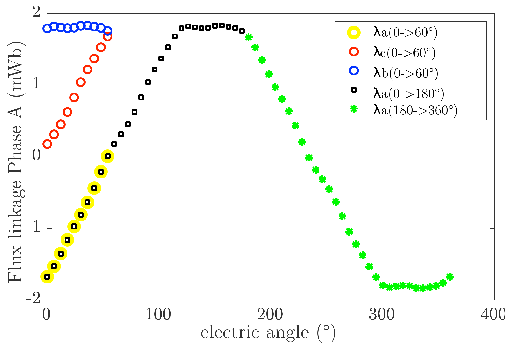
Reconstruction of Flux Linkage
We would like to reconstruct the flux linkage of “phase a” over a full period of 360° electrical degrees, from the evaluation of the magnetic flux of the three “phases a, b, c,” over an interval of 60° electrical degrees (Figure 6). The flux linkages have an electrical periodicity of , corresponding to a mechanical periodicity of .

Figure 6.
Flux linkages reconstruction.
The Fourier series decomposition of the flux linkages of the three phases is given by:
where:
- n is the number of the n-th harmonic
- is the angular position of the rotor in electrical degrees.
- is the phase shift of the n-th harmonic of the flux linkage.
- is the amplitude of the n-th harmonic of the flux linkage.
The reconstruction of phase A flux linkage is made by following the two steps:
Step 1: This step allows the reconstitution of the flux linkage of phase A over 180° electrical degrees range from the evaluation of the flux linkage of the three phases over 60° electrical degrees range.
Let , with .
If °,
Then .
By setting We obtain:
Therefore .
is a data vector of over the interval
In the similar way, we can prove that:
By concatenation, we have:
Step 2: The flux linkage is 180 electrical degrees anti-periodic.
Thus
Reconstruction of Magnetic Induction at the Stator
For iron losses evaluation, we need normal and tangential components of the magnetic induction in each mesh element over a period of 360° electrical degrees. The reconstruction of magnetic induction vector is slightly different from the method used for reconstructing the linkage. Indeed, magnetic induction is a vector and local quantity unlike flux linkage, which is a scalar and global quantity. To reconstruct the magnetic induction in the machine, we proceed as follows:
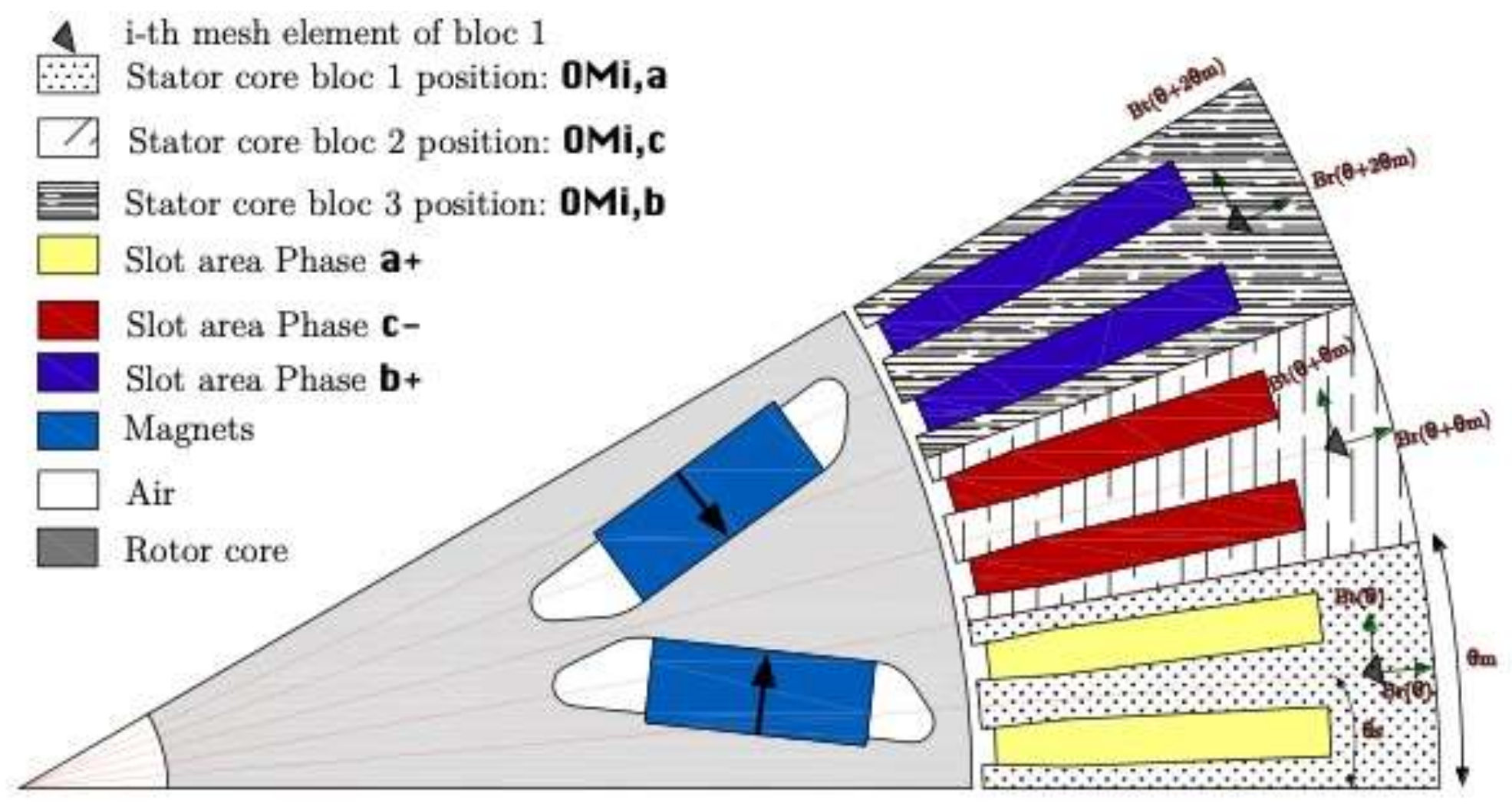
Step 1: At first, we divide the stator of one pole into three blocks (block 1, block 2, block 3) respectively containing the slots of “phase a+” (input of phase a), “phase c-“ (output of phase c), “phase b+” (input of phase b). Block 2 and block 3 are geometrically phase shifted with respect to block 1 by respectively 60°/p mechanical degrees and 120°/p mechanical degrees. The aim of this work is to reconstruct the magnetic induction of each mesh element of block 1 over a complete period of 360° electrical degrees from the calculation of the magnetic induction of block 1, block 2 and block 3 over 60° electrical degrees. For each i-th mesh element of block 1, we associate with it a position and a magnetic induction vector . The magnetic induction is obtained from the matrix containing the magnetic induction vectors of all mesh elements of the machine.
For et
interior stator diameter
exterior stator diameter
The machine meshing is a random process. Therefore, it is not certain that the position of the i-th mesh element of block 2, corresponds to the position of the i-th mesh element of block 1 after rotation by an angle of 60°/p mechanical degrees. To have the same numbering of the mesh elements for block 1, block 2 and block 3, we calculate the positions of the mesh elements of block 2 and block 3 after rotation of the positions of the mesh elements of block 1 by 60°/p mechanical degrees and 120°/p mechanical degrees (Figure 7):
- is the complex number:
- is the complex operator of rotation of center (0,0) and angle .

Figure 7.
V-shaped synchronous machine test with 6 pole pairs.
Figure 7.
V-shaped synchronous machine test with 6 pole pairs.
The magnetic induction of block 2 and block 3 are extracted from the matrix B containing the magnetic induction vectors of all mesh elements of the machine and of all the positions of the mesh elements of these different blocks ( et ).
We have the magnetic induction of the mesh elements of block 1 (, block 2 (, and block 3 (, over a range of electrical degrees.
Step 2: This step reconstructs the magnetic induction of block 1 () over an interval of electrical degrees from the magnetic induction and calculated over a . electrical degree. The periodicity of the magnetic flux for a mesh element of block 1 for different rotor positions is 360° electrical degrees. Thus, we can write the Fourier series decomposition of the radial and tangential components of the magnetic flux for the i-th mesh element of block 1 by:
The i-th mesh element of block 2 in rotation of 60°/p mechanical degrees with respect to the i-th mesh element of block 1 will have the same magnetic induction as that of the i-th mesh element of block 1 phase shifted by 60° electrical degrees. To have the vector expression of the magnetic induction of block 2, it is necessary to consider the mechanical rotation mechanical degree that the magnetic induction of block 1 to block 2 undergoes. Thus, we have for block 2, the following relation:
In a similar way for block 3, we have:
Let with .
If ,
Then
By setting
Therefore
Similarly, for the tangential component, we have:
Thus, the relation between the vector magnetic inductions of block 1 and block 2 is given by:
By using the same approach as the calculation of vector magnetic induction of block 2, we can show that the vector magnetic induction of block 3 obeys the following relation:
The magnetic induction of block on an interval of 180° electrical degrees is:
The magnetic induction is 180° electrical degrees anti-periodic. Thus, the magnetic induction over an interval of 360° electrical degrees is given by (Figure 8):
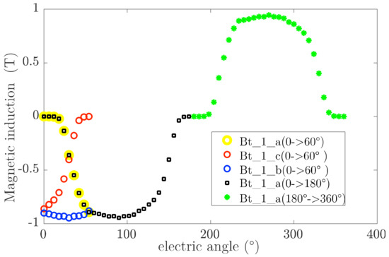
Figure 8.
Tangential magnetic induction reconstruction into mesh element “1”.
Iron Loss Calculation
From the waveform phase flux linkages, magnetic induction vector reconstructed, we can compute the induced voltage and the core losses.
The iron loss calculation is based on the iron Bertotti loss model in its integral form:
The core losses are performed by computing the tangential magnetic induction and radial magnetic induction in each mesh element of the stator and the rotor lamination. The total iron loss is the contribution of hysteresis losses, eddy current losses and excess losses [19].
with , the poles number.
2.3.2. Fixed Rotor Position (DQ Model)
With the objective to reduce the FE computation time, the analysis of the three-phase machines is simplified by using the classical theory of synchronous machines based on Park’s transformation which allows a change of variables of electrical quantities, such as flux linkages, voltages and currents. The electrical quantities in the reference frame , fixed to the stator are sinusoidal in time, while the electrical quantities in the rotating reference frame are constants.
The classical dq theory is built based on two assumptions:
- (a)
- The windings are sinusoidal on the stator periphery. Then, the flux linkages and induce voltage have sinusoidal variation.
- (b)
- The magnetic circuit is linear.
The mean torque is given in dq frame by:
In the classical theory of dq transformation, the d and q axis are uncoupled (no cross-coupling effect) and the flux linkage in dq axis is independent of rotor position . But for high torque density machines, especially for the design of “interior permanent magnet motor”, the magnetic circuit may be saturable so that we cannot neglect the cross-coupling effect of d and q axis. A lot of works have been done by taking into account the cross-coupling effect to have better performances evaluation [20,21,22,23,24,25]. In that case, the flux linkage expressions are:
The dq model developed in this paper is based on finite-element calculation and considers the cross-coupling effect of dq axis. Based on the first harmonic hypothesis, the flux linkages should be constant into dq axis for each rotor position. Thus, we would only need one rotor position to evaluate the flux linkages, compute the voltage and the mean torque of the machine. However, the winding supply at a high-speed in the weakening region may not be sine-distributed and due to high rank harmonics created by slots at the stator, the flux linkages of each phase are not sinusoidal.
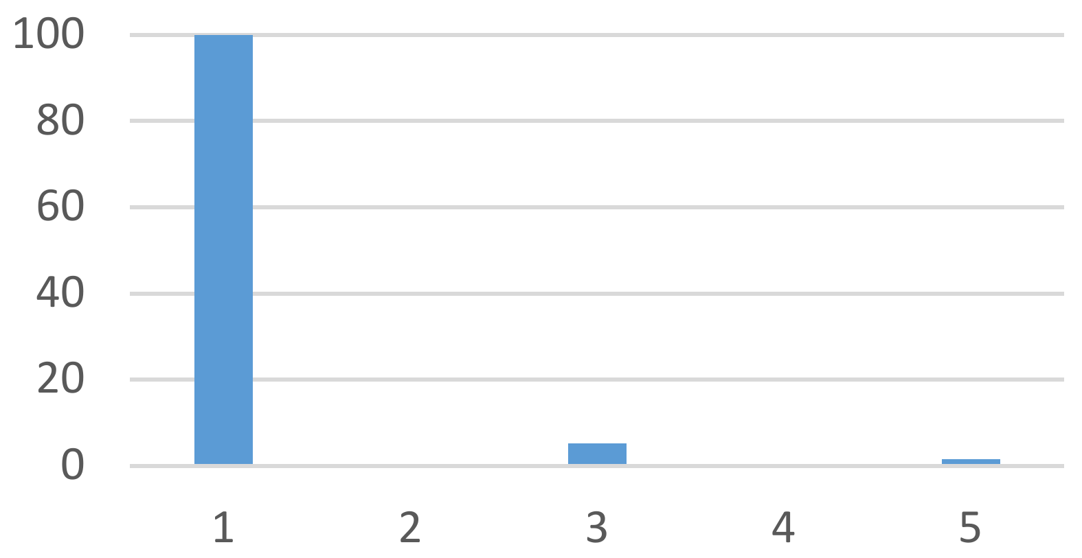
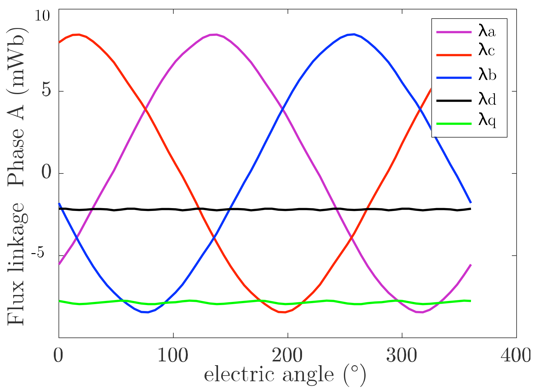
The harmonic content of the no-load flux linkage of our test machine is shown on Figure 9. The harmonics of orders 3 and 5 represent respectively 5% and 1.5% of fundamental value. The flux linkages of “phases a, b, c” can be considered as a sinus. The flux linkage in the d and q axis is almost constant and doesn’t depend on the rotor position (Figure 10).

Figure 9.
No load flux linkage harmonics “1, 2, 3” in percent with respect to harmonic 1.
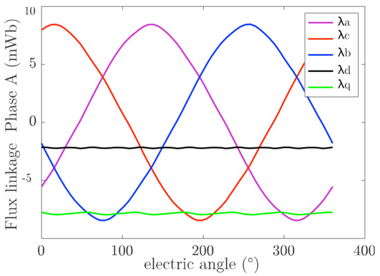
Figure 10.
No load flux linkage vs. rotor position.
To increase the speed of the machine, we have to reduce the flux linkage to respect the voltage constraints. As the machine is supplied by three-phases sinusoidal currents, reducing the flux linkage by varying the torque angle control from its optimal value to 90° electrical degrees, will mainly decrease the fundamental component of flux linkage. We can see in Figure 11, the first harmonic of the flux linkage decreases with increasing angle control . However, the harmonics of ranks 3 and 5 remain almost unchanged when increases.
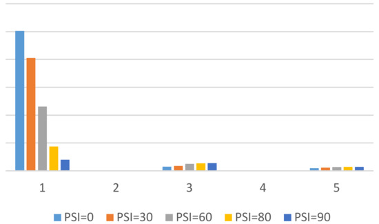
Figure 11.
Flux linkage harmonics “1, 3, 5” vs. angle control (ψ°).
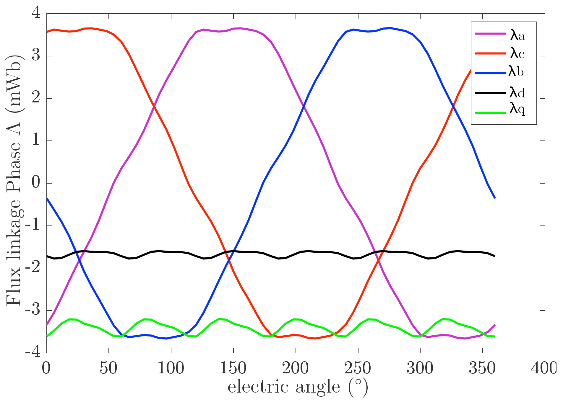
When the supply control angle increases, the percentage of high-order harmonics (3rd and 5th) relative to the fundamental increases (Figure 12). Thus for the weakening angle of 80°, the values of the harmonics 3 and 5 represent respectively 31% and 16% of the fundamental of flux linkage. The flux linkage of the three phases “a,b,c” can no longer be considered sinuous. The flux linkages in the d and q axis are not constant Figure 13.
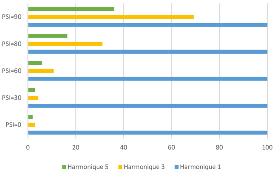
Figure 12.
Percent of harmonics “3,5” with respect to the harmonic “1” vs. angle control (ψ).
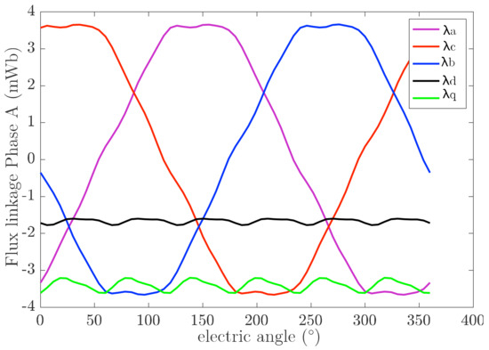
Figure 13.
Flux linkage vs. rotor position for ψ = 70°.
In the case the flux linkage in dq axis is not constant, we must consider the dependency of rotor position:
The use of only one rotor position, as is the case in the bibliography to evaluate the performances of the machine is therefore not accurate. Thus, depending on the rotor position of the machine, the performances such as the induced voltage and the average torque of the rotor will be overestimated or underestimated.
To solve this problem, we decided to increase the number of rotor positions allowing the calculation of electrical quantities. To build the multi-static “abc model” with the proposed methodology, we used 10 rotor positions to evaluate the electromagnetic performances of the machine. For “dq model”, we want to use as few as possible to compute the induced voltage and average torque while having better accuracy compared to the reference “abc model”. Then, we used two rotor positions to compute the performances of the machine. Indeed, the use of two positions allows us to have a “dq model” 5 times faster than the multi-static “abc model” with a relative difference of less than 5% on the calculation of average torque and induced voltage. However, the “dq model” has some drawbacks such as that it does not allow the evaluation of the torque ripples, eddy current losses of magnets at the rotor.
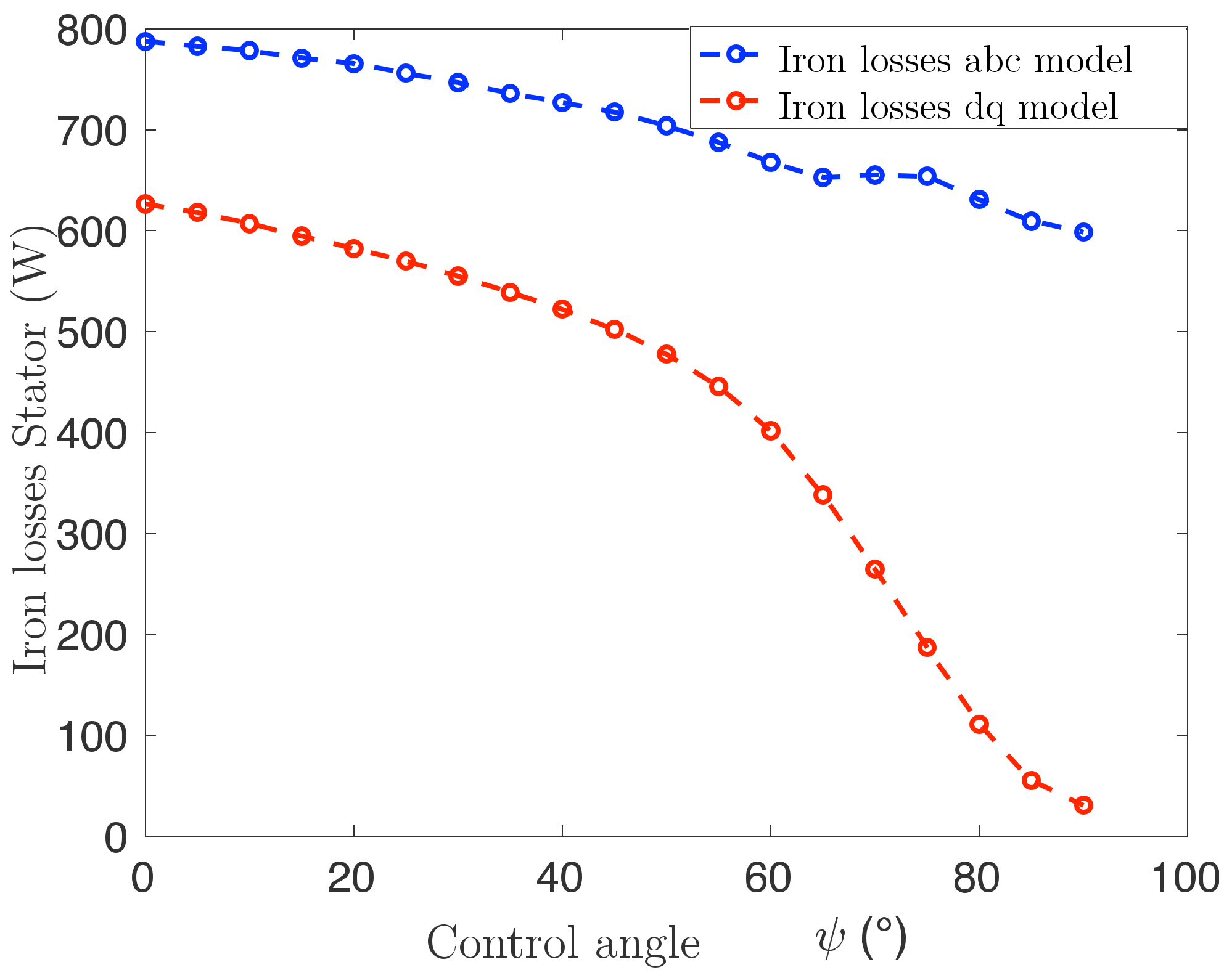
The iron loss calculations based on the first harmonic hypothesis is not accurate and give a relative deviation from the “abc model” greater than 70% at high control angle (Figure 14).
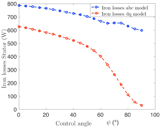
Figure 14.
Comparison of iron stator losses with the “abc model” vs. “dq model”.
3. Optimization Results
To see the influence that the choice of electromagnetic model could have on the sizing of an electrical machine, we optimized a synchronous magnet machine using the two developed electromagnetic models (“abc model” and “dq model”). The proposed “dq model” using two rotor positions has the advantage of being at least 5 times faster than the “abc model”, with good accuracy for torque and induced voltage evaluations. However, this model is based on the first harmonic hypothesis and does not allow the computation of losses in magnets and iron losses with good accuracy. The optimization also considers mechanical stress at high speed. The machine topology chosen for this optimization is a synchro-reluctant double-layer V-shaped permanent magnet machine.
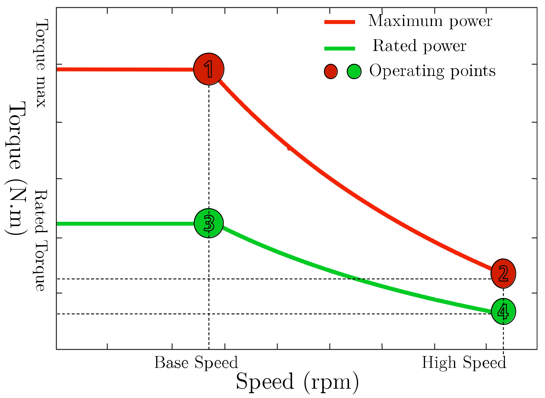
The machine has been optimized on 4 operating points: 2 on maximum power characteristic and 2 on rated power (Figure 15).

Figure 15.
Electric motor torque-speed characteristic.
We choose 4 operating points to have a reasonable computation time for optimization (Figure 15).
The objective functions of this optimization are:
- -
- Maximize the torque at operating point 1
- -
- Minimize the average total loss of operating points 3 and 4 of the rated power: .
- -
- Minimize the total mass of the machine
The chosen optimization algorithm is the NSGA III [26] from PlatEmo [14]. The machine was optimized under constraints of torque, active length, outer diameter, inverter current and voltage limitations. This voltage is limited to the maximum voltage that can be supplied by the battery via the inverter. The maximum voltage that can be supplied by the inverter is [19]:
where:
- : Sinusoidal Pulse With Modulation;
- : Space Vector Pulse With Modulation;
- The maximum Neutral-Phase Voltage;
- The battery voltage.
The geometric and power supply constraints are summarized in the specifications of Table 2. The number of optimization variables is 37 with 29 geometric variables for the topology with 2 magnet layers and 8 control variables for supply.
Table 2.
Motor design specifications.
The optimization algorithm chosen is the NSGA III. We considered an initial population of 300 individuals over 250 generations. This corresponds to the assessment of 75,000 individuals. The machine used is an Intel® Xeon® CPU X5690 @ 3.47GHz with 40 cores. The computation time for the optimization using the “dq model” is 15 h, while the optimization using the “abc model” is 75 h.
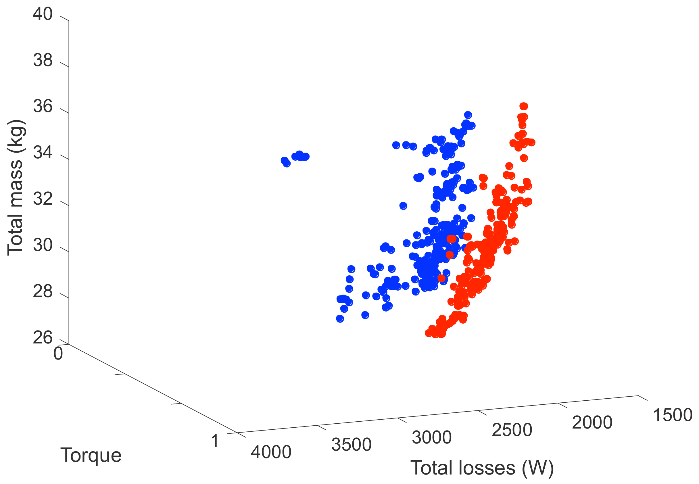
The Pareto Fronts of the two optimizations are shown in Figure 16. We represented the three objectives of optimization over a two-dimensional graph. The x-axis corresponds to the maximization of the torque, the y-axis corresponds to the minimization of the average total loss at points 3 and 4, and the third objective corresponds to the minimization of the total mass. The mass is represented by a color gradient from blue to yellow. By analyzing the two Pareto Fronts, we notice that the range of the mass (28 kg to 38 kg) is roughly the same for the two optimizations.
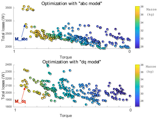
Figure 16.
Pareto Front of optimization results with “abc model” and “dq model”.
The superposition of the two Pareto Fronts is presented in Figure 17. For greater readability, we presented in Figure 18 the Pareto front comparison in 2D graph by fixing the motor mass into the range [34 kg; 34.3 kg]. The losses generated by the machines obtained from the optimization using the “dq model” are less than the losses from the machines obtained with the “abc model”. This difference is because the iron loss model used by the “dq model” is based on the first harmonic hypothesis (Figure 14). This model therefore tends to underestimate the iron losses of the machine. We decided to compare two machines obtained through these optimizations with a comparison of their geometry and performances. The machines M_abc and M_dq have the same maximum torque and substantially the same mass (37 kg and 35 kg).

Figure 17.
Pareto Front comparison: “abc model” vs. “dq model”.
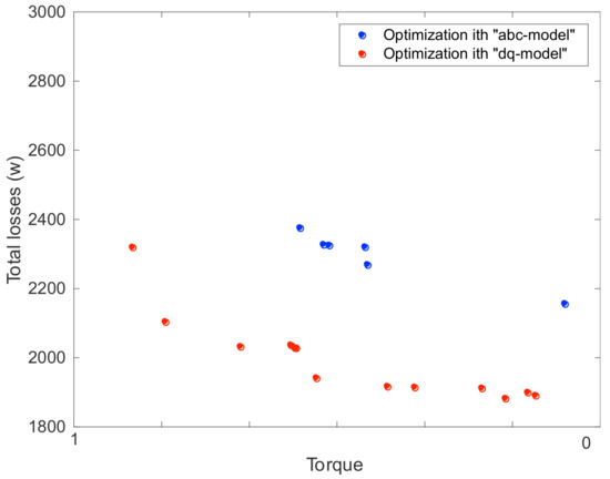
Figure 18.
Pareto Front for machines with 34 kg: “abc model” vs. “dq model”.
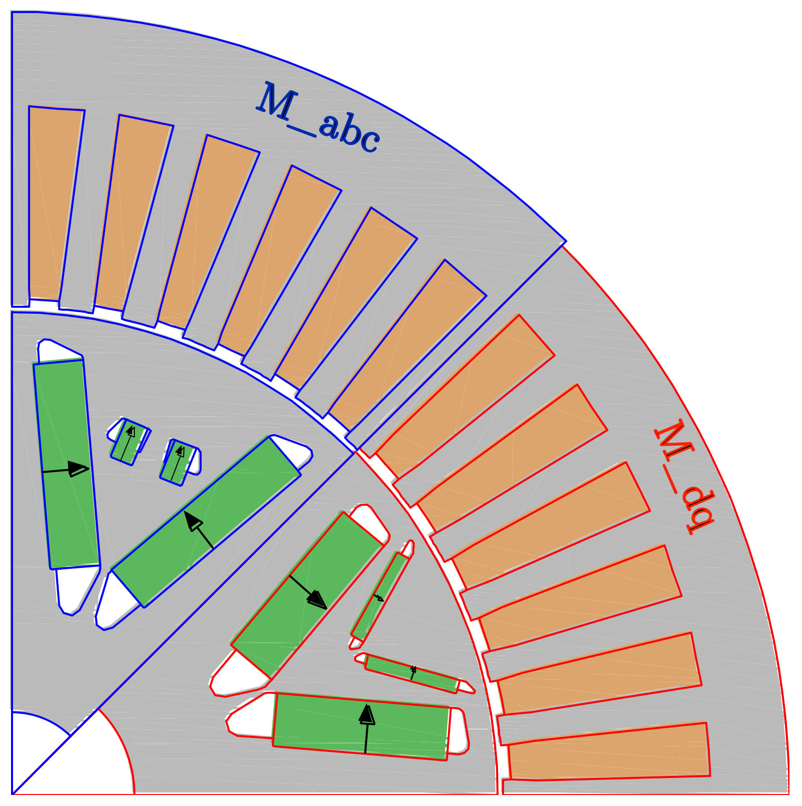
Figure 19 shows the geometry of the two machines M_abc and M_dq. We notice that these two machines have roughly the same geometries, such as the exterior stator diameter, the active length (164 mm and 162 mm) and the air gap radius. The arrangement of the magnets on the rotor is different for the two machines. Table 3 compares the performances of the two machines computed from electromagnetic “abc model”. The M-dq machine has more copper losses and more iron losses (evaluated by “abc model”) than the M_abc machine. The high iron losses of M_dq machine can be explained by the fact that the loss calculation model used by the “abc model” is more precise than the “dq model”. It seems that for this application, a machine optimized from a more precise loss model tend to have fewer losses than an optimized machine with less precise loss model.
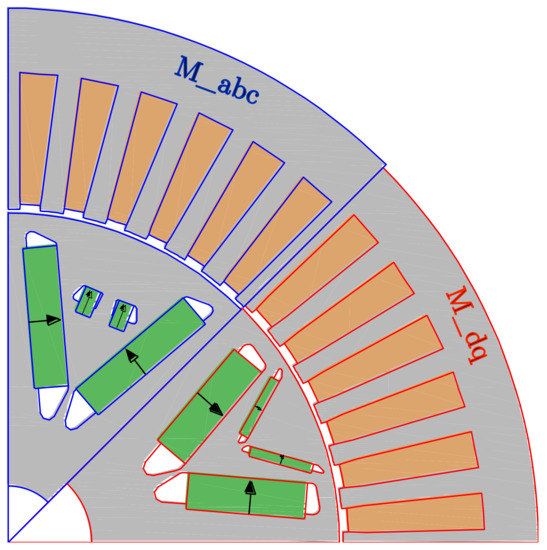
Figure 19.
Optimized machines with the “dq model” and the “abc model”.
Table 3.
Comparison of machines obtained after optimization m_abc vs. m_dq.
The thicknesses of the teeth and the thickness of the stator yoke of the machine M_abc is about 15% greater than those of the teeth and stator yoke of the machine M_dq. Therefore, the machine M_abc has less local saturation than the machine M_dq. Hence the iron losses of the M_abc machine are lower than those of the M_dq machine. The copper losses of the M_dq machine are greater than those of the M_abc machine because the M_dq machine has more copper and the same maximum current as the M_abc machine.
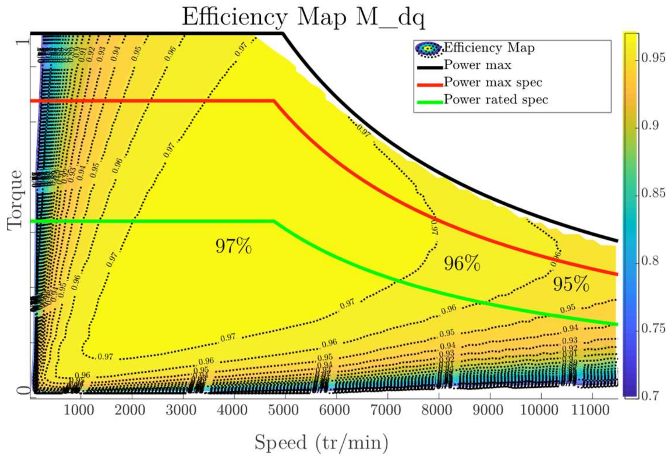
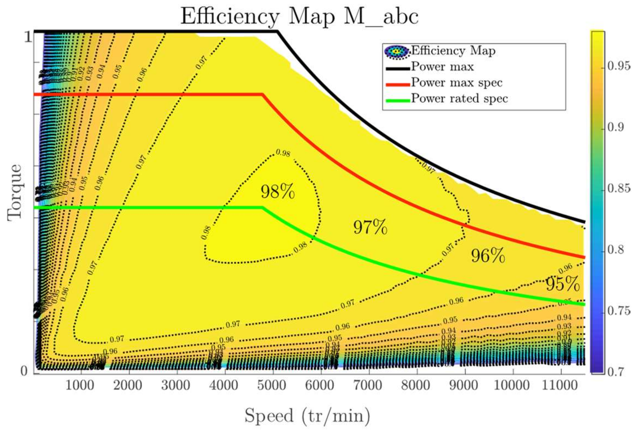
We drew the efficiency maps of the two machines obtained after optimization from the two electromagnetic models “dq model” and “abc model” respectively in and Figure 20 and Figure 21. The electromagnetic performances necessary for the mapping of these two machines were evaluated based on the “abc model”. The two machines obtained have interesting performances with a large efficiency zone at 97%. The peak efficiency of the M_abc machine is 98%, while that of M_dq is 97%. The use of a less accurate and faster electromagnetic “dq model” allows obtaining a machine with good performances in the torque-speed map. The use of the “abc model” in the optimization process results in a machine with better performances than the machine obtained with the “dq model”. The 97% and 96% efficiency area are extended for high-speed operating points with the machine obtained with “abc model”.

Figure 20.
Efficiency map for the machine optimized by the “dq model”.

Figure 21.
Efficiency map for the machine optimized by the “abc model”.
Therefore, it could be found that the choice of the electromagnetic model during the optimization process has indeed an influence on the geometry and performances of the machine obtained after the optimization. Thus, during an optimization process, we will use a “dq model” to get quick results and get an idea of the possible machine solutions for a given specification. A more precise and therefore longer optimization can be achieved by using the “abc model” in two different ways. The first is to start an optimization in “dq model” by initializing the starting population with the one obtained during the last evaluation of the optimization with the “dq model”. The second method is to use an “abc model” optimization directly without initializing the population.
4. Conclusions
This article allowed us to present a multi-objective optimization method for designing a multi-layer synchro-reluctant machine based on finite element calculation models. We studied two models of electromagnetic calculations (“dq model” and “abc model”). To reduce the overall optimization computation time, we analyzed the influences of “dq model”, which is five times faster than the electromagnetic “abc model” during the optimization process. This study showed that the choice of the electromagnetic “dq model” or “abc model” has a real impact on the final geometry and performances of the machine. The “abc model” allows obtaining a machine with better performances with efficiency zones at 97% and 98% wider than the machine obtained with the use of the electromagnetic “dq model”. This result is mainly due to the difference of iron losses of “abc model” and “dq model”. Thus, the use of the electromagnetic “dq model” will allow a faster optimization and to have an idea of the possible solutions for a given specification. For the sizing of a more accurate machine, it is necessary to use the electromagnetic “abc model” which is five times longer in terms of computation time.
Author Contributions
K.M.C., S.H., M.B., G.M.R., M.G. and Y.C. have equally contributed to this manuscript. All authors have read and agreed to the published version of the manuscript.
Funding
This research received no external funding.
Institutional Review Board Statement
Not applicable.
Informed Consent Statement
Not applicable.
Data Availability Statement
The data presented in this study are available on request from the corresponding author.
Conflicts of Interest
The authors declare no conflict of interest.
References
- Castagnaro, E.; Bacco, G.; Bianchi, N. Rotor Iron Losses in High-Speed Synchronous Reluctance Motors. In Proceedings of the 2018 XIII International Conference on Electrical Machines (ICEM), Alexandroupoli, Greece, 3–6 September 2018; pp. 1310–1316. [Google Scholar] [CrossRef]
- Stipetic, S.; Miebach, W.; Zarko, D. Optimization in design of electric machines: Methodology and workflow. In Proceedings of the 2015 Intl Aegean Conference on Electrical Machines & Power Electronics (ACEMP), Side, Turkey, 2–4 September 2015; pp. 441–448. [Google Scholar] [CrossRef]
- Degano, M.; Di Nardo, M.; Galea, M.; Gerada, C.; Gerada, D. Global design optimization strategy of a synchronous reluctance machine for light electric vehicles. In Proceedings of the IET Conference Proceedings, Edinburgh, UK, 7 March 2016; p. 5. [Google Scholar] [CrossRef]
- Han, W.; van Dang, C.; Kim, J.W.; Kim, Y.J.; Jung, S.Y. Global-Simplex Optimization Algorithm Applied to FEM-Based Optimal Design of Electric Machine. IEEE Trans. Magn. 2017, 53, 2015–2018. [Google Scholar] [CrossRef]
- Sarigiannidis, A.G.; Beniakar, M.E.; Kladas, A.G. Fast Adaptive Evolutionary PM Traction Motor Optimization Based on Electric Vehicle Drive Cycle. IEEE Trans. Veh. Technol. 2017, 66, 5762–5774. [Google Scholar] [CrossRef]
- Li, Q.; Fan, T.; Li, Y.; Guo, J.; Wen, X. Design and Optimization of Permanent Magnet Synchronous Machines for Driving Cycle. In Proceedings of the 2019 IEEE Vehicle Power and Propulsion Conference (VPPC), Hanoi, Vietnam, 14–17 October 2019; pp. 1–5. [Google Scholar] [CrossRef]
- Barcaro, M.; Bianchi, N.; Magnussen, F. Permanent-magnet optimization in permanent-magnet-assisted synchronous reluctance motor for a wide constant-power speed range. IEEE Trans. Ind. Electron. 2012, 59, 2495–2502. [Google Scholar] [CrossRef]
- Grunditz, E.A.; Thiringer, T. Electric Vehicle Acceleration Performance and Motor Drive Cycle Energy Efficiency Trade-Off. In Proceedings of the 2018 23rd Conference on Electrical Machines, Alexandroupoli, Greece, 3–6 September 2018; pp. 717–723. [Google Scholar]
- Carraro, E.; Morandin, M.; Bianchi, N. Optimization of a traction PMASR motor according to a given driving cycle. In Proceedings of the 2014 IEEE Transportation Electrification Conference and Expo (ITEC), Chicago, IL, USA, 23–25 June 2014; pp. 1–6. [Google Scholar] [CrossRef]
- Cardoso, J.F.; Chillet, C.; Gerbaud, L.; Belhaj, L.A. Electrical Machine Design by optimization for E-motor Application: A Drive Cycle Approach. In Proceedings of the 2020 International Conference on Electrical Machines (ICEM), Gothenburg, Sweden, 23–26 August 2020; pp. 2514–2519. [Google Scholar] [CrossRef]
- Li, Q.; Fan, T.; Wen, X.; Li, Y.; Wang, Z.; Guo, J. Design optimization of interior permanent magnet synchronous machines for traction application over a given driving cycle. In Proceedings of the IECON 2017-43rd Annual Conference of the IEEE Industrial Electronics Society, Beijing, China, 29 October–1 November 2017; pp. 1900–1904. [Google Scholar] [CrossRef]
- Günther, S.; Ulbrich, S.; Hofmann, W. Driving cycle-based design optimization of interior permanent magnet synchronous motor drives for electric vehicle application. In Proceedings of the 2014 International Symposium on Power Electronics, Electrical Drives, Automation and Motion, Ischia, Italy, 18–20 June 2014; pp. 25–30. [Google Scholar] [CrossRef]
- Crozier, R.; Mueller, M. A new MATLAB and octave interface to a popular magnetics finite element code. In Proceedings of the 2016 22nd International Conference on Electrical Machines, ICEM 2016, Lausanne, Switzerland, 4–7 September 2016; pp. 1251–1256. [Google Scholar]
- Tian, Y.; Cheng, R.; Zhang, X.; Jin, Y. PlatEMO: A MATLAB Platform for Evolutionary Multi-Objective Optimization [Educational Forum]. IEEE Comput. Intell. Mag. 2017, 12, 73–87. [Google Scholar] [CrossRef] [Green Version]
- Lei, G.; Zhu, J.; Guo, Y. Multidisciplinary Design Optimization Methods for Electrical Machines and Drive Systems; Springer: Berlin, Germany, 2016. [Google Scholar]
- Murthy, C.A. Genetic Algorithms: Basic principles and applications. In Proceedings of the 2012 2nd National Conference on Computational Intelligence and Signal Processing (CISP), Chongqind, China, 16–18 October 2012; p. 22. [Google Scholar]
- Chehouri, A.; Younes, R.; Khoder, J.; Perron, J.; Ilinca, A. A Selection Process for Genetic Algorithm Using Clustering Analysis. Algorithms 2017, 10, 123. [Google Scholar] [CrossRef] [Green Version]
- Holland, J.H. Adaptation in Natural and Artificial Systems: An Introductory Analysis with Applications to Biology, Control and Artificial Intelligence; MIT Press: Cambridge, MA, USA, 1992. [Google Scholar]
- Cissé, K.M.; Hlioui, S.; Cheng, Y.; Belhadi, M.; Gabsi, M. Optimization of V-shaped Synchronous Motor for Automotive Application. In Proceedings of the 2018 XIII International Conference on Electrical Machines (ICEM), Alexandroupoli, Greece, 3–6 September 2018; pp. 906–912. [Google Scholar] [CrossRef]
- Bianchi, N. Electrical Machine Analysis Using Finite Elements; Taylor & Francis Group: Oxford, UK, 2005. [Google Scholar]
- Bianchi, N.; Bolognani, S. Magnetic models of saturated Interior Permanent Magnet motors based on Finite Element Analysis. In Proceedings of the Conference Record of 1998 IEEE Industry Applications Conference, Thirty-Third IAS Annual Meeting (Cat. No. 98CH36242), St. Louis, MO, USA, 12–15 October 1998; Volume 1, pp. 27–34. [Google Scholar]
- Goss, J.; Mellor, P.H.; Wrobel, R.; Staton, D.A.; Popescu, M. The design of AC permanent magnet motors for electric vehicles: A computationally efficient model of the operational envelope. In Proceedings of the 6th IET International Conference on Power Electronics, Machines and Drives (PEMD 2012), Bristol, UK, 27–29 March 2012; pp. 1–6. [Google Scholar] [CrossRef] [Green Version]
- Štumberger, G.; Polajžer, B.; Štumberger, B.; Toman, M.; Dolinar, D. Evaluation of experimental methods for determining the magnetically nonlinear characteristics of electromagnetic devices. IEEE Trans. Magn. 2005, 41, 4030–4032. [Google Scholar] [CrossRef]
- Wang, S.; Degano, M.; Kang, J.; Galassini, A.; Gerada, C. A Novel Newton-Raphson-Based Searching Method for the MTPA Control of Pmasynrm Considering Magnetic and Cross Saturation. In Proceedings of the 2018 23rd International Conference on Electrical Machines (ICEM), Alexandroupoli, Greece, 3–6 September 2018; pp. 1360–1366. [Google Scholar]
- Zhou, C.; Huang, X.; Fang, Y.; Wu, L. Comparison of PMSMs with Different Rotor Structures for EV Application. In Proceedings of the 2018 23rd International Conference on Electrical Machines (ICEM), Alexandroupoli, Greece, 3–6 September 2018; pp. 609–614. [Google Scholar]
- Deb, K.; Jain, H. An Evolutionary Many-Objective Optimization Algorithm Using Reference-Point-Based Nondominated Sorting Approach, Part I: Solving Problems with Box Constraints. IEEE Trans. Evol. Comput. 2014, 18, 577–601. [Google Scholar] [CrossRef]


Publisher’s Note: MDPI stays neutral with regard to jurisdictional claims in published maps and institutional affiliations. |
© 2021 by the authors. Licensee MDPI, Basel, Switzerland. This article is an open access article distributed under the terms and conditions of the Creative Commons Attribution (CC BY) license (https://creativecommons.org/licenses/by/4.0/).