Optimal Chiller Loading by Team Particle Swarm Algorithm for Reducing Energy Consumption

Abstract

Energy saving is an important issue for multiple-chiller systems. Optimal chiller loading (OCL) in multiple-chiller systems has been investigated with many optimization algorithms to save energy. Particle swarm optimization (PSO) algorithm has been successful in solving this problem in some cases, but not in all. This study innovatively added a team evolution to the original particle swarm optimization algorithm, called team particle swarm optimization (TPSO). The TPSO enhances the effectiveness of original particle swarm optimization to better solve the OCL problem. The TPSO algorithm is composed of two evolutions: particle evolution and team evolution. The partial load ratio (PLR) of each operating chiller and the on-off state of each chiller are the particle evolution parameters and team evolution parameters, respectively. To evaluate the performance of the proposed method, this paper adopts three case studies so the results generated from the proposed algorithm TPSO, the original particle swarm optimization (PSO) and other recently published algorithms can be compared. In these three case studies, the optimal results generated by using TPSO algorithm are the same as those by other compared algorithms. In case 1 under 5717 RT and 5334 RT cooling load, the results generated using the TPSO are lower than those by the original PSO in the amounts of 63.35 and 79.33 kW, respectively. The results indicated that the TPSO algorithm not only enabled the optimal solution in minimizing energy consumption, but also demonstrated the best stability when compared to other algorithms. In conclusion, the presented TPSO algorithm is an efficient and promising new algorithm for solving the OCL problem.

1. Introduction

Air conditioning systems contributes considerably to the energy consumption in buildings—with their chiller systems being the main cause of energy consumption. Different operation strategies for the chiller systems result in significant differences in the energy used. An optimal chiller loading (OCL) method proposed by Chang [1], alongside many other algorithms, aimed to find the optimal on-off state and partial loading ratio (PLR) of each chiller to minimize the energy consumption. Chang [1] used the Lagrangian method to investigate the optimal loading ratio of each chiller to minimize the energy consumption at different cooling loads in two cases. The result showed that while the setup PLR value of the Lagrangian method saved much energy compared to the equal loading rate of traditional methods, the Lagrangian algorithm suffered a flaw in an inability to converge at low demands. Subsequently, Chang [2] proposed a genetic algorithm to overcome the flaw of the Lagrangian algorithm. However, as a result, the optimal energy consumption of genetic algorithm increased by about 0.4% compared to the Lagrangian method. Lee and Lin [3] considered that the constraint of chiller PLR cannot be less than 0.3 and used the particle swarm optimization (PSO) algorithm to investigate the OCL problem. The results showed that the PSO has performed well in the two tested cases with three-chiller and four-chiller systems.

In recent years, various algorithms have been developed for different applications; some of them have been applied to solve the OCL problem successfully. Chang et al. [4,5,6] used simulated annealing and evolution strategy; Ardakani et al. [7] and Chen et al. [8] applied particle swarm optimization. Lee et al. [9] and Lin et al. [10] adopted differential evolution (DE) and two-stage differential evolution; Coelho et al. [11,12] applied differential cuckoo search approach and improved firefly algorithm. Sulaiman et al. [13] adopted differential search; Duan et al. [14] used teaching-learning-based optimization. Salari et al. [15] adopted general algebraic modeling system; Teimourzadeh et al. [16] applied augmented group search optimization algorithm. Xu et al. [17] used improved grasshopper optimization algorithm; Qi et al. [18] adopted improved fruit fly optimization (IFOA) algorithm. Farnaz et al. [19] applied exchange market algorithm; Yu [20] used distributed chaotic estimation of distribution algorithm (DCEDA). Lin [21] adopted modified artificial bee colony algorithm; Zheng et al. [22] applied improved invasive weed optimization (EIWO) algorithm. SUN et al. [23] used an equilibrium optimization algorithm. PSO and its improved version have also been used to solve the daily optimal chiller load problem and the optimal chiller sequencing problem. Beghi et al. [24] and ABALLA et al. [25] applied PSO and Fuzzified PSO respectively to discuss the optimal chiller sequencing operation within a year. Askarzadeh et al. [26] adopted two improved PSO to optimize daily electrical power consumption in multi-chiller systems. On the other hand, CITRONI et al. [27] studied on an array configuration of rectified optical nanoantennas for energy harvesting application.

Based on these studies, the DE, IFOA, DCEDA and EIWO algorithms have shown their efficacy on finding the best solution and stability in three well-known cases on 3-, 4- and 6-chiller systems. On the other hand, the PSO algorithm has shown efficacy as the best solution in two of the three cases on the 3-chiller and 4-chiller systems but not the 6-chiller system. Under the two cases of 5717 RT and 5334 RT cooling load on the 6-chiller system, the best solutions of energy consumption generated by using the PSO [3] are higher than those by the IFOA [18] and EIWO [22] in the amounts of 63.35 and 79.33 kW, respectively. In this current study, an improved particle swarm optimization algorithm, called team particle swarm optimization (TPSO), is proposed to enhance the performance of the original particle swarm optimization to best solve the OCL problem. The TPSO algorithm is composed of two evolutions: particle evolution and team evolution. The partial load ratio (PLR) of each operating chiller and the on-off state of each chiller are the particle evolution parameter and team evolution parameter, respectively. To evaluate the performance of the proposed TPSO algorithm, the paper adopts three case studies so the results of the proposed TPSO algorithm can be compared with the original PSO algorithm along with other recently published algorithms.

The remainder of this paper is organized as follows. Section 2 describes the OCL problem of multiple-chiller systems. Section 3 introduces the evolution mechanism of TPSO algorithm. Section 4 compares the results of case studies. Section 5 is the conclusions.

2. System Description

An OCL problem in a typical multi-chiller system is shown in Figure 1 [28]. The system includes chillers, cooling coils, valves, and pumps. A bypass pipe is used to balance the chilled water flow between the primary and secondary chilled water system. The cooling load is provided by each chiller operated independently.

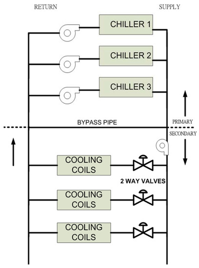
Figure 1. Decoupled system of a multiple-chiller system [28].

The best solution is when the sum of energy consumption of each chiller is minimized while the load is satisfied. The energy consumption of a centrifugal chiller is a convex function of its PLR for a given wet-bulb temperature [2]:

$$Powe{r}_i=a_i+b_i\ast PL{R}_i+c_i\ast PL{R}_i^2+d_i\ast PL{R}_i^3$$

(1)

where a_i, b_i, c_i, d_i are coefficients of power curve of i^th chiller.

The objective of solving the OCL problem is to minimize the summation of energy consumption of each chiller, as shown in Equation (2):

$$J=Min{\displaystyle \sum _{i=1}^{l}Powe{r}_i}$$

(2)

The first constraint of OCL problem is that the summation of cooling provided by each chiller should meet the system cooling load, as shown in Equation (3)

$${\displaystyle \sum _{i=1}^{l}PL{R}_i\ast Q_i}=CL$$

(3)

where Q_i = capacity of ith chiller, CL = system cooling load.

The other constraint is that the partial load of each operated chiller cannot be smaller than 30% [3], as shown in Equation (4)

$$PL{R}_i\ge 0.3$$

(4)

3. Method

The original particle swarm optimization (PSO) algorithm is proposed by Kennedy and Eberhart [29,30], and it moves the position of particles to find the optimal solution. The position of the particle is referred to the value of parameter. The progress of optimization is to move the particle position toward the personal best position and the best position of all particles. The number of iterations decides the end of evolution. The PSO evolution rule is showed as follows:

$$v_{i,k+1}=w·v_{i,k}+c_1·r_1·\left(P{b}_{i,k}-x_{i,k}\right)+c_2·r_2·\left(Gb-x_{i,k}\right)$$

(5)

$$x_{i,k+1}=x_{i,k}+v_{i,k+1}$$

(6)

where v_i represents the velocity of particle i, k means the iteration number, w represents inertial weight, c₁ and c₂ are acceleration constants, r₁ and r₂ are two random values in the range of [0, 1], x_i,k represents the current position of particle i, Pb_i is the position of particle i with personal best solution and Gb is the position of the particle with best solution found thus far.

The PSO algorithm and the improved versions have been successfully applied in several fields. However, the PSO algorithm was the best solution for the OCL problem in some cases but not all. In order to improve on the efficacy of the original PSO algorithm, a new concept of team and model best solutions are added to the PSO algorithm for evolution. The improved algorithm is named as team particle swarm optimization (TPSO). In TPSO, the particles are allocated to several teams. Particles in the same team have the same on-off state of each chiller. The TPSO algorithm is composed of two evolutions: particle evolution and team evolution. Particle evolution progresses on every evolutionary generation. Team evolution progresses after particle evolution has made a number of progressions. The partial load ratio (PLR) of each operating chiller and the on-off state of each chiller are particle evolution parameter and team evolution respectively. The particle evolution in the TPSO algorithm is different from the original particle evolution in the PSO, in that the progress of optimization is to move the particle position toward the personal best position, team best position, and model best position. The best team position is the best position of particles in the same team, and the model best position is the best position of all particles with the same on-off state as each chiller.

The evolution formula of particle evolution of TPSO is presented as follows:

$$v_{i,k+1}=w{v}_{i,k}+c_1\ast r_1\ast \left(P{b}_{i,k}-x_{i,k}\right)+c_2\ast r_2\ast \left(T{b}_{i,k}-x_{i,k}\right)+c_3\ast r_3\ast \left(M{b}_{i,k}-x_{i,k}\right)$$

(7)

$$x_{i,k+1}=x_{i,k}+v_{i,k+1}$$

(8)

where Tb_i means the position of particle which has the best performance in the same team with particle i, Mb_i means the position of particle which has the best performance in the same on-off state as each chiller with particle i thus far.

The process of team evolution is: first, a random value is given as r₄, and then r₄ is compared with the evolution threshold. If r₄ meets the conditions for change in the on-off state of chillers, the state of chillers in the team will change and the personal best position of each particle in this team, and best team position, will be reinitialized.

The evolution rule of team evolution is as follows

$$\{\begin{array}{c}{r}_4<Th{r}_l,s_{i,k+1} = s_{i,k} \mathrm{for} \mathrm{each} \mathrm{chiller} i\\ r_4>Th{r}_l \mathrm{and} r_4<Th{r}_l,s_{i,k+1} = \mathrm{rand}(0,1) \mathrm{reinitialize} \mathrm{ecah} \mathrm{chiller}i\\ r_4>Th{r}_l,s_{i,k+1} = Gb{s}_k \mathrm{for} \mathrm{each} \mathrm{chiller} i\end{array}$$

(9)

$$s_i=\{\begin{array}{c}1,\mathrm{chiller} \mathrm{state} \mathrm{is} \mathrm{on}\\ 0,\mathrm{chiller} \mathrm{state} \mathrm{is} \mathrm{off}\end{array}$$

(10)

where $r_4$ is the random value between 0 and 1, $Th{r}_l$ and $Th{r}_h$ are the threshold values for device state evolution. Gbs_k means the chiller state of the best particle founded thus far.

The progress of the TPSO evolution is presented in the flowchart of Figure 2, and the scudo code is shown in Figure 3. A case of six particles and two teams for a 3-chiller system is used to describe the evolution process. At step 1, the particles are assigned to teams in sequence, as shown in Table 1. Particle 1, 2, 3 are belong to team 1 and Particle 4,5,6 are belong to team 2. At step 2, the on-off states of chillers in each team are initialized, as shown in Table 2. The chiller on-off states of particles in team 1 are the same, chiller 1 is off, chiller 2 is on and chiller 3 is on. The on-off states of chiller 1, 2 and 3 of particles in team 2 are on, off, and on, respectively. At step 3, the parameter value, PLR, of each chiller are initialized to meet the system cooling load, as shown in Table 3. At step 4, the particle evolution for PLR of each chiller starts, as shown in Table 4. At step 5, the team evolution for on-off states of chillers starts, as shown in Table 5. The random value of $r_4$ for team1 is 0.3 at this evolution, therefore the on-off states of chiller 1, 2 and 3 of particles in team 1 are not changed; the $r_4$ for team2 is 0.5, therefore the on-off states and PLR of chiller 1, 2 and 3 of particles in team 2 are reinitialized.

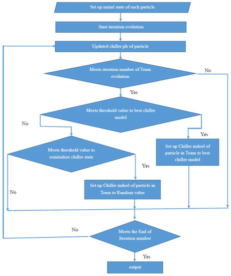
Figure 2. Flow Chart of the TPSO evolution progress.

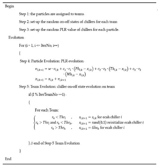
Figure 3. Pseudo-code of the TPSO algorithm.

Table 1. Step 1: the particles are assigned to teams.

Particle No	Team No	Chiller1 State	Chiller2 State	Chiller3 State	Chiller1 PLR	Chiller2 PLR	Chiller3 PLR
1	1
2	1
3	1
4	2
5	2
6	2

Table 2. Step 2: set up the random on-off states of chillers for each team.

Particle No	Team No	Chiller1 State	Chiller2 State	Chiller3 State	Chiller1 PLR	Chiller2 PLR	Chiller3 PLR
1	1	0	1	1
2	1	0	1	1
3	1	0	1	1
4	2	1	0	1
5	2	1	0	1
6	2	1	0	1

Table 3. Step 3: set up the random PLR value of chillers for each particle.

Particle no	Team no	Chiller1 state	Chiller2 state	Chiller3 state	Chiller1 PLR	Chiller2 PLR	Chiller3 PLR
1	1	0	1	1	0	0.5	0.5
2	1	0	1	1	0	0.3	0.7
3	1	0	1	1	0	0.2	0.8
4	2	1	0	1	0.6	0	0.4
5	2	1	0	1	0.5	0	0.5
6	2	1	0	1	0.7	0	0.3

Table 4. Step 4: the particle evolution for PLR of each chiller (on-off state of chillers is not changed).

Particle No	Team No	Chiller1 State	Chiller2 State	Chiller3 State	Chiller1 Plr	Chiller2 Plr	Chiller3 Plr
1	1	0	1	1	0	0.52	0.58
2	1	0	1	1	0	0.34	0.66
3	1	0	1	1	0	0.25	0.75
4	2	1	0	1	0.63	0	0.37
5	2	1	0	1	0.41	0	0.59
6	2	1	0	1	0.72	0	0.28
Particle No	Team No	Chiller1 State	Chiller2 State	Chiller3 State	Chiller1 Plr	Chiller2 Plr	Chiller3 Plr
1	1	0	1	1	0	0.58	0.52
2	1	0	1	1	0	0.34	0.66
3	1	0	1	1	0	0.35	0.65
4	2	1	0	1	0.60	0	0.40
5	2	1	0	1	0.41	0	0.59
6	2	1	0	1	0.52	0	0.48

Table 5. Step 5: the team evolution for on-off states of chillers.

Particle No	Team No	Chiller1 State	Chiller2 State	Chiller3 State	Chiller1 PLR	Chiller2 PLR	Chiller3 PLR
1	1	0	1	1	0	0.42	0.58
2	1	0	1	1	0	0.34	0.66
3	1	0	1	1	0	0.25	0.75
4	2	1	0	1	0.63	0	0.37
5	2	1	0	1	0.41	0	0.59
6	2	1	0	1	0.72	0	0.28
Particle No	Team No	Chill1 State	Chiller2 State	Chiller3 State	Chiller1 PLR	Chiller2 PLR	Chiller3 PLR
1	1	0	1	1	0	0.42	0.58
2	1	0	1	1	0	0.34	0.66
3	1	0	1	1	0	0.25	0.75
4	2	1	1	0	0.33	0.67	0
5	2	1	1	0	0.49	0.51	0
6	2	1	1	0	0.66	0.34	0

4. Case Study

In this case study, three well-known cases of multiple-chiller systems, shown in Table 6, are utilized to compare the performance of the TPSO algorithm, the original PSO, and recently published algorithms, i.e., (DE) [9], (IFOA) [18], (DCEDA) [20], and (EIWO) [22]. Case 1 [22] includes four 1280 RT and two 1250 RT chillers; Case 2 [2] contains two 1000 RT and two 450 RT chillers; Case 3 [2] consists of three 800 RT chillers. The performance coefficients of the chillers are listed in Table 6.

Table 6. Coefficients of power curve of chillers in 3 cases.

System	Chiller	ai	bi	ci	di	Capacity (RT)
Case 1	CH-1	399.345	−122.120	770.460	0.000	1280
	CH-2	287.116	80.040	700.480	0.000	1280
	CH-3	−120.505	1525.990	−502.140	0.000	1280
	CH-4	−19.121	898.760	−98.150	0.000	1280
	CH-5	−95.029	1202.390	−352.160	0.000	1250
	CH-6	191.750	224.860	524.040	0.000	1250
Case 2	CH-1	104.090	166.570	−430.130	512.530	450
	CH-2	−67.150	1177.790	−2174.530	1456.530	450
	CH-3	384.710	−779.130	1151.420	−63.200	1000
	CH-4	541.630	413.480	−3626.500	4021.410	1000
Case 3	CH-1	100.950	818.610	−973.430	788.550	800
	CH-2	66.598	606.340	−380.580	275.950	800
	CH-3	130.090	304.500	14.377	99.800	800

4.1. Parameter Analysis

The optimal parameter values of TPSO in the OCL problem are discussed with two examples, Case 1 with cooling load 6096RT and Case 3 with 2160RT. The results are shown in Table 7 and Table 8. The performance of the TPSO can be obtained by setting the following parameter values: the total particle number is 200, and the particle number of a team is 5, which means of 40 teams. The inertial weight is 0.4, and the acceleration constants are 1. The iteration numbers in particle and team evolutions are 500 and 30, respectively. Therefore, these parameter values are used for the following case studies.

Table 7. Parameter analysis for six chillers with cooling load of 6096 RT in Case 1.

Particle Number	Particle Number in a Team	Iteration Number of Team	Low Threshold	High Threshold	Initial Weight	Accelerate Constant	Min	Max	Average	Max-Min	Standard Deviation
200	5	30	0.4	0.9	0.4	1	4143.706	4143.706	4143.706	1.66 × 10−5	2.46 × 10−6
200	10	30	0.4	0.9	0.4	1	4143.706	4143.706	4143.706	6.77 × 10−6	1.58 × 10−6
100	5	30	0.4	0.9	0.4	1	4143.706	4143.709	4143.706	2.56 × 10−3	3.63 × 10−4
200	5	30	0.2	0.9	0.4	1	4143.706	4143.706	4143.706	1.07 × 10−5	1.75 × 10−6
200	5	30	0.4	0.8	0.4	1	4143.706	4143.706	4143.706	6.90 × 10−6	1.39 × 10−6
200	5	50	0.4	0.9	0.4	1	4143.706	4143.706	4143.706	6.31 × 10−5	1.02 × 10−5
200	5	30	0.4	0.9	0.6	1	4143.706	4143.706	4143.706	6.31 × 10−5	1.02 × 10−5
200	5	30	0.4	0.9	0.4	1.2	4143.706	4143.706	4143.706	6.31 × 10−5	1.02 × 10−5

Table 8. Parameter analysis for 3 chillers with cooling load of 2160 RT in Case 3.

Particle Number	Particle Number in a Team	Iteration Number of Team	Low Threshold	High Threshold	Initial Weight	Accelerate Constant	Min	Max	Average	Max-Min	Standard Deviation
200	5	30	0.4	0.9	0.4	1	1583.807	1583.807	1583.807	1.16 × 10−6	1.69 × 10−7
200	10	30	0.4	0.9	0.4	1	1583.807	1583.807	1583.807	5.99 × 10−6	1.37 × 10−6
100	5	30	0.4	0.9	0.4	1	1583.807	1583.807	1583.807	1.83 × 10−5	3.13 × 10−6
200	5	30	0.2	0.9	0.4	1	1583.807	1583.807	1583.807	1.31 × 10−6	2.46 × 10−7
200	5	30	0.4	0.8	0.4	1	1583.807	1583.807	1583.807	3.49 × 10−6	5.05 × 10−7
200	5	50	0.4	0.9	0.4	1	1583.807	1583.807	1583.807	6.30 × 10−7	1.20 × 10−7
200	5	30	0.4	0.9	0.6	1	1583.807	1583.807	1583.807	1.53 × 10−7	3.39 × 10−8
200	5	30	0.4	0.9	0.4	1.2	1583.807	1583.807	1583.807	2.06 × 10−7	4.80 × 10−8

4.2. Performance of TPSO

For testing the performance of TPSO, the results of Cases 1 to 3 under various cooling loads (40%, 50%, 60%, 70%, 75%, 80%, 85%, 90%) are presented in Table 9, Table 10 and Table 11, respectively. The results are carried out for 50 independent runs and the parameter values are shown in Table 12.

Table 9. Power Consumption of chillers in case 1 operated by TPSO algorithm.

CL (RT)	PLR of Chiller (Case Min)						Power (kW)
	Chi 1	Chi 2	Chi 3	Chi 4	Chi 5	Chi 6	Min	Max	Average	Max-Min	Standard Deviation
6858 (90%)	0.813	0.750	1	1	1	0.839	4738.575	4738.575	4738.575	0.000	0.000
6477 (85%)	0.728	0.656	1	1	1	0.717	4421.649	4421.649	4421.649	0.000	0.000
6096 (80%)	0.643	0.563	1	1	1	0.594	4143.706	4143.706	4143.706	0.000	0.000
5717 (75%)	0	0.715	1	1	1	0.793	3842.553	3842.553	3842.553	0.000	0.000
5334 (70%)	0	0.583	1	1	1	0.622	3546.437	3546.437	3546.437	0.000	0.000

Table 10. Power Consumption of chillers in Case 2 operated by TPSO algorithm.

CL (RT)	PLR (Case Min)				Power (kW)
	Chi 1	Chi 2	Chi 3	Chi 4	Min	Max	Average	Max-Min	Standard Deviation
2610 (90%)	0.991	0.906	1	0.756	1857.299	1857.299	1857.299	0.000	0.000
2320 (80%)	0.829	0.806	0.897	0.688	1455.665	1455.665	1455.665	0.000	0.000
2030 (70%)	0.726	0.740	0.722	0.649	1178.137	1178.137	1178.137	0.000	0.000
1740 (60%)	0.604	0.658	0.565	0.608	998.533	998.533	998.533	0.000	0.000
1450 (50%)	0.607	0	0.568	0.609	820.073	820.073	820.073	0.000	0.000
1160 (40%)	0	0	0.555	0.605	651.072	651.072	651.072	0.000	0.000

Table 11. Power Consumption of chillers in case 3 operated by TPSO algorithm.

CL (RT)	PLR (Case Min)			Power (kW)
	Chiller 1	Chiller 2	Chiller 3	Min	Max	Average	Max-Min	Standard Deviation
2160 (90%)	0.725	0.975	1	1583.807	1583.807	1583.807	0.000	0.000
1920 (80%)	0.659	0.859	0.882	1403.196	1403.196	1403.196	0.000	0.000
1680 (70%)	0.596	0.745	0.759	1244.325	1244.325	1244.325	0.000	0.000
1440 (60%)	0	0.885	0.915	993.602	993.602	993.602	0.000	0.000
1200 (50%)	0	0.743	0.757	832.325	832.325	832.325	0.000	0.000
960 (40%)	0	0.570	0.630	692.251	692.251	692.251	0.000	0.000

Table 12. Evolution parameters chosen for TPSO algorithm.

Parameter	Value
Particle number	200
Particle number in a team	5
Iteration number	500
Iteration number for a team evolution	30
inertial weight	0.4
acceleration constant	0.4
the low threshold value of model evolution	0.4
the high threshold value of model evolution	1

The difference between maximum and minimum values and standard deviations also shows zero to the third decimal. This information indicates the high stability of the TPSO algorithm under the chosen evolution parameters. The power consumptions of each cooling load under each case operated by TPSO algorithm with respect to the iteration number are presented in Figure 4, Figure 5 and Figure 6. These results indicated that the TPSO algorithm also has been effective with convergence in each cooling load of each case.

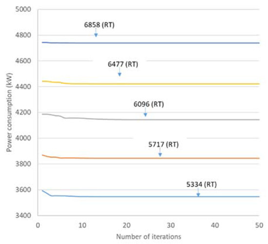
Figure 4. Power consumptions of chillers in Case 1 operated by TPSO algorithm.

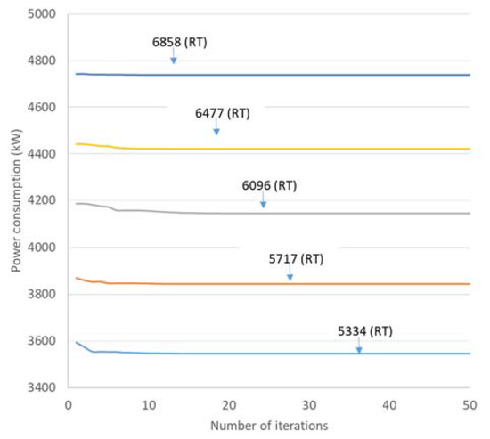
Figure 5. Power consumptions of chillers in Case 2 operated by TPSO algorithm.

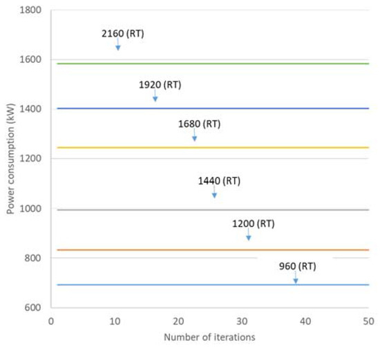
Figure 6. Power consumptions of chillers in Case 3 operated by TPSO algorithm.

4.3. Compare the TPSO Algorithm with Other Algorithms

To verify the effectiveness of the TPSO algorithm as the best solution, three case studies are adopted to compare the results of the proposed algorithm with original particle swarm optimization and other recently published algorithms, DE [9], DCEDA [20], EIWO [22] and IFOA [18]. The compared results for Case 1, Case 2, and Case 3 are shown in Table 13, Table 14 and Table 15, respectively.

Table 13. Comparison of optimum value operated by TPSO, PSO, DCEDA, EIWO, IFOA in Case 1.

CL (RT)	PSO [22]	DCEDA [20]	EIWO [22]	IFOA [18]	Best Solution of Compared Method	TPSO	C-A (kW)	C-B (kW)
	Power (kW) (A)	Power (kW)	Power (kW)	Power (kW)	Power (kW) (B)	Power (kW) (C)
6858 (90%)	4738.58	4738.58	4738.575	4738.575	4738.575	4738.575	0.00	0.00
6477 (85%)	4421.65	4421.65	4421.649	4421.649	4421.649	4421.649	0.00	0.00
6096 (80%)	4143.71	4143.71	4143.706	4143.706	4143.706	4143.706	0.00	0.00
5717 (75%)	3905.90	3843.07	3842.553	3842.553	3842.553	3842.553	−63.35	0.00
5334 (70%)	3625.77	3546.48	3546.438	3546.437	3546.437	3546.437	−79.33	0.00

Table 14. Comparison of optimum value operated by TPSO, PSO, DE, EIWO, IFOA in Case 2.

CL (RT)	PSO [3]	DE [9]	EIWO [22]	IFOA [18]	Best Solution of Compared Method	TPSO	C-A (kW)	C-B (kW)
	Power (kW) (A)	Power (kW)	Power (kW)	Power (kW)	Power (kW) (B)	Power (kW) (C)
2610 (90%)	1857.30	1857.30	1857.30	1857.30	1857.30	1857.30	0.00	0.00
2320 (80%)	1455.66	1455.66	1455.66	1455.66	1455.66	1455.66	0.00	0.00
2030 (70%)	1178.14	1178.14	1178.14	1178.14	1178.14	1178.14	0.00	0.00
1740 (60%)	998.53	998.53	998.53	998.53	998.53	998.53	0.00	0.00
1450 (50%)	820.07	820.07	820.07	820.07	820.07	820.07	0.00	0.00
1160 (40%)	651.07	651.07	651.07	651.07	651.07	651.07	0.00	0.00

Table 15. Comparison of optimum value operated by PSO, DE, EIWO, IFOA and best known solution in Case 3.

CL (RT)	PSO [3]	DE [9]	EIWO [22]	IFOA [18]	Best Solution of Compared Method	TPSO	C-A (kW)	C-B (kW)
	Power (kW) (A)	Power (kW)	Power (kW)	Power (kW)	Power (kW) (B)	Power (kW) (C)
2160 (90%)	1583.81	1583.81	1583.81	1583.81	1583.81	1583.81	0.00	0.00
1920 (80%)	1403.20	1403.20	1403.20	1403.20	1403.20	1403.20	0.00	0.00
1680 (70%)	1244.32	1244.32	1244.32	1244.32	1244.32	1244.32	0.00	0.00
1440 (60%)	993.60	993.60	993.60	993.60	993.60	993.60	0.00	0.00
1200 (50%)	832.33	832.33	832.33	832.33	832.33	832.33	0.00	0.00
960 (40%)	692.25	692.25	692.25	692.25	692.25	692.25	0.00	0.00

In these three case studies, the results generated by using TPSO algorithm are the same with those by other algorithms. In Case 1, the compared algorithms are original PSO [22], DCEDA [20], EIWO [22] and IFOA [18] as shown on Table 13; In Case 2 and Case 3 the original PSO [3], DE [9], EIWO [22] and IFOA [18] are compared, as shown on Table 14 and Table 15, respectively. In Case 1 under 5717 RT and 5334 RT cooling load, the results generated by using the TPSO are lower than those by the original PSO in the amounts of 63.35 and 79.33 kW, respectively. The comparison indicated that the TPSO algorithm out-performed the original PSO algorithm and all other algorithms presented in this paper.

4.4. Comparison of Stability

To compare the stability of TPSO witha number of other algorithms, the maximum, minimum, and average difference between maximum and minimum, and standard deviation of power consumption of chillers under various cooling loads in Cases 1 to 3 are presented in Table 16, Table 17 and Table 18. The algorithms selected for comparison are IFOA [18] and DCEDA [20]. The difference between the maximum and minimum values and standard deviations of the TPSO algorithm in all cases are shown in zero to the third decimal, as indicated in these three tables. It is demonstrative that the TPSO algorithm yields the best stability when compared with IFOA and DCEDA.

Table 16. Comparison of stability yielded by TPSO, IFOA and DCEDA in Case 1.

CL (RT)	Method	Power (kW)				Standard Deviation
		Max	Min	Average	Max-Min
6858 (90%)	TPSO	4738.575	4738.575	4738.575	0.000	0.000
	IFOA [18]	4738.577	4738.575	4738.576	0.002	0.001
	DCEDA [20]	4739.08	4738.58	4738.66	0.5	0.113
6477 (85%)	TPSO	4421.649	4421.649	4421.649	0.000	0.000
	IFOA [18]	4421.651	4421.649	4421.649	0.002	0.001
	DCEDA [20]	4422.83	4421.65	4421.78	1.18	0.232
6096 (80%)	TPSO	4143.706	4143.706	4143.706	0.000	0.000
	IFOA [18]	4143.708	4143.706	4143.707	0.002	0.001
	DCEDA [20]	4144.31	4143.71	4143.78	0.6	0.116
5717 (75%)	TPSO	3842.553	3842.553	3842.553	0.000	0.000
	IFOA [18]	3844.036	3842.553	3842.652	1.483	0.395
	DCEDA [20]	3845.16	3842.55	3842.85	2.61	0.557
5334 (70%)	TPSO	3546.437	3546.437	3546.437	0.000	0.000
	IFOA [18]	3546.438	3546.437	3546.437	0.001	0.001
	DCEDA [20]	3562.39	3546.44	3547.09	15.950	2.338

Table 17. Comparison of stability yielded by TPSO, IFOA and DCEDA in Case 2.

CL(RT)	Method	Power (kW)				Standard Deviation
		Max	Min	Mean	Max-Min
2610 (90%)	TPSO	1857.299	1857.299	1857.299	0.000	0.000
	IFOA [18]	1857.299	1857.299	1857.299	0.000	0
	DCEDA [18]	1858.62	1857.3	1857.43	1.32	0.314
2320 (80%)	TPSO	1455.665	1455.665	1455.665	0.000	0.000
	IFOA [18]	1455.665	1455.665	1455.665	0.000	0
	DCEDA [18]	1457.41	1455.66	1455.77	1.75	0.283
2030 (70%)	TPSO	1178.137	1178.137	1178.137	0.000	0.000
	IFOA [18]	1178.137	1178.137	1178.137	0.000	0
	DCEDA [18]	1178.72	1178.14	1178.2	0.58	0.096
1740 (60%)	TPSO	998.533	998.533	998.533	0.000	0.000
	IFOA [18]	998.533	998.533	998.533	0.000	0
	DCEDA [18]	1000.56	998.53	998.61	2.03	0.627
1450 (50%)	TPSO	820.073	820.073	820.073	0.000	0.000
	IFOA [18]	820.073	820.073	820.073	0.000	0
	DCEDA [18]	822.36	820.07	820.24	2.29	0.463
1160 (40%)	TPSO	651.072	651.072	651.072	0.000	0.000
	IFOA [18]	651.072	651.072	651.072	0.000	0
	DCEDA [18]	656.72	651.09	651.35	5.63	1.708

Table 18. Comparison of stability yielded by TPSO, IFOA and DCEDA in Case 3.

CL(RT)	Method	Power(kW)				Standard Deviation
		Max	Min	Mean	Max-Min
2160 (90%)	TPSO	1583.807	1583.807	1583.807	0.000	0.000
	IFOA [18]	1583.807	1583.807	1583.807	0.000	0
	DCEDA [20]	1585.24	1583.81	1583.98	1.43	0.295
1920 (80%)	TPSO	1403.196	1403.196	1403.196	0.000	0.000
	IFOA [18]	1403.196	1403.196	1403.196	0.000	0
	DCEDA [20]	1405.01	1403.20	1403.32	1.81	0.272
1680 (70%)	TPSO	1244.325	1244.325	1244.325	0.000	0.000
	IFOA [18]	1244.325	1244.325	1244.325	0.000	0
	DCEDA [20]	1244.83	1244.32	1244.37	0.51	0.087
1440 (60%)	TPSO	993.602	993.602	993.602	0.000	0.000
	IFOA [18]	993.602	993.602	993.602	0.000	0
	DCEDA [20]	995.07	993.60	993.66	1.47	0.209
1200 (50%)	TPSO	832.325	832.325	832.325	0.000	0.000
	IFOA [18]	832.325	832.325	832.325	0.000	0
	DCEDA [20]	834.30	832.33	832.42	1.97	0.316
960 (40%)	TPSO	692.251	692.251	692.251	0.000	0.000
	IFOA [18]	692.251	692.251	692.251	0.000	0
	DCEDA [20]	695.22	692.25	692.39	2.97	0.485

5. Conclusions

This study proposed an improved particle swarm optimization algorithm, called team particle swarm optimization (TPSO), to enhance the performance of the original PSO to better solve the OCL problem. To verify the effectiveness of the TPSO algorithm, figures from three case studies are adopted so comparison can be made on the TPSO algorithm, the PSO algorithm, and other recently published algorithms. In these three case studies, the optimal results generated by using TPSO algorithm are the same as those by other compared algorithms. In case 1 under 5717 RT and 5334 RT cooling load, the results generated by using the TPSO are lower than those by the original PSO in the amounts of 63.35 and 79.33 kW, respectively. The comparison results indicate that the TPSO algorithm not only enables the optimal solution in minimizing energy consumption, but also demonstrates the best stability when compared to other algorithms. Therefore, the presented TPSO algorithm is an efficient new algorithm in optimal chiller loading problem and has the potential to be further applied to solve various optimal problems.

References

- Chang, Y.-C. A novel energy conservation method—Optimal chiller loading. Electr. Power Syst. Res. 2004, 69, 221–226. [Google Scholar] [CrossRef]
- Chang, Y.-C.; Lin, J.-K.; Chuang, M.-H. Optimal chiller loading by genetic algorithm for reducing energy consumption. Energy Build. 2005, 37, 147–155. [Google Scholar] [CrossRef]
- Lee, W.-S.; Lin, L.-C. Optimal chiller loading by particle swarm algorithm for reducing energy consumption. Appl. Therm. Eng. 2009, 29, 1730–1734. [Google Scholar] [CrossRef]
- Chang, Y.-C.; Chen, W.-H.; Lee, C.-Y.; Huang, C.-N. Simulated annealing based optimal chiller loading for saving energy. Energy Convers. Manag. 2006, 47, 2044–2058. [Google Scholar] [CrossRef]
- Chang, Y.-C. Optimal chiller loading by evolution strategy for saving energy. Energy Build. 2007, 39, 437–444. [Google Scholar] [CrossRef]
- Chang, Y.-C.; Lee, C.-Y.; Chen, C.-R.; Chou, C.-J.; Chen, W.-H.; Chen, W.-H. Evolution strategy based optimal chiller loading for saving energy. Energy Convers. Manag. 2009, 50, 132–139. [Google Scholar] [CrossRef]
- Ardakani, A.J.; Ardakani, F.F.; Hosseinian, S. A novel approach for optimal chiller loading using particle swarm optimization. Energy Build. 2008, 40, 2177–2187. [Google Scholar] [CrossRef]
- Chen, C.-L.; Chang, Y.-C.; Chan, T.-S. Applying smart models for energy saving in optimal chiller loading. Energy Build. 2014, 68, 364–371. [Google Scholar] [CrossRef]
- Lee, W.-S.; Chen, Y.-T.; Kao, Y. Optimal chiller loading by differential evolution algorithm for reducing energy consumption. Energy Build. 2011, 43, 599–604. [Google Scholar] [CrossRef]
- Lin, C.-M.; Wu, C.-Y.; Tseng, K.-Y.; Ku, C.-C.; Lin, S.-F. Applying two-stage differential evolution for energy saving in optimal chiller loading. Energies 2019, 12, 622. [Google Scholar] [CrossRef] [Green Version]
- Dos Santos Coelho, L.; Klein, C.E.; Sabat, S.L.; Mariani, V.C. Optimal chiller loading for energy conservation using a new differential cuckoo search approach. Energy 2014, 75, 237–243. [Google Scholar] [CrossRef]
- Dos Santos Coelho, L.; Mariani, V.C. Improved firefly algorithm approach applied to chiller loading for energy conservation. Energy Build. 2013, 59, 273–278. [Google Scholar] [CrossRef]
- Sulaiman, M.H.; Ibrahim, H.; Daniyal, H.; Mohamed, M.R. A new swarm intelligence approach for optimal chiller loading for energy conservation. Proc. Soc. Behav. Sci. 2014, 129, 483–488. [Google Scholar] [CrossRef] [Green Version]
- Duan, P.-Y.; Li, J.-Q.; Wang, Y.; Sang, H.-Y.; Jia, B.-X. Solving chiller loading optimization problems using an improved teaching-learning-based optimization algorithm. Optim. Control. Appl. Methods 2018, 39, 65–77. [Google Scholar] [CrossRef]
- Salari, E.; Askarzadeh, A. A new solution for loading optimization of multi-chiller systems by general algebraic modeling system. Appl. Therm. Eng. 2015, 84, 429–436. [Google Scholar] [CrossRef]
- Teimourzadeh, H.; Jabari, F.; Mohammadi-Ivatloo, B. An augmented group search optimization algorithm for optimal cooling-load dispatch in multi-chiller plants. Comput. Electr. Eng. 2020, 85, 106434. [Google Scholar] [CrossRef]
- Wenhan, X.; Yuanxing, W.; Di, Q.; Rouyendegh, B.D. Improved grasshopper optimization algorithm to solve energy consuming reduction of chiller loading. Energy Sour. Part A Recover. Util. Environ. Eff. 2019, 1–14. [Google Scholar] [CrossRef]
- Qi, M.-Y.; Li, J.-Q.; Han, Y.-Y.; Dong, J.-X. Optimal chiller loading for energy conservation using an improved fruit fly optimization algorithm. Energies 2020, 13, 3760. [Google Scholar] [CrossRef]
- Sohrabi, F.; Nazari-Heris, M.; Mohammadi-Ivatloo, B.; Asadi, S. Optimal chiller loading for saving energy by exchange market algorithm. Energy Build. 2018, 169, 245–253. [Google Scholar] [CrossRef]
- Yu, J.; Liu, Q.; Zhao, A.; Qian, X.; Zhang, R. Optimal chiller loading in HVAC system using a novel algorithm based on the distributed framework. J. Build. Eng. 2020, 28, 101044. [Google Scholar] [CrossRef]
- Lin, C.-M.; Tseng, K.-Y.; Lin, S.-F. Optimal chiller loading using modified artificial bee colony algorithm. Sens. Mater. 2020, 32, 2387. [Google Scholar] [CrossRef]
- Zheng, Z.-X.; Li, J.-Q. Optimal chiller loading by improved invasive weed optimization algorithm for reducing energy consumption. Energy Build. 2018, 161, 80–88. [Google Scholar] [CrossRef]
- Sun, F.; Yu, J.; Zhao, A.; Zhou, M. Optimizing multi-chiller dispatch in HVAC system using equilibrium optimization algorithm. Energy Rep. 2021, 7, 5997–6013. [Google Scholar] [CrossRef]
- Beghi, A.; Cecchinato, L.; Cosi, G.; Rampazzo, M. A PSO-based algorithm for optimal multiple chiller systems operation. Appl. Therm. Eng. 2012, 32, 31–40. [Google Scholar] [CrossRef]
- Abdalla, E.A.H.; Nallagownden, P.; Nor, N.M.; Romlie, M.F.; Abdalsalam, M.E.; Muthuvalu, M.S. Intelligent approach for optimal energy management of chiller plant using fuzzy and PSO techniques. In Proceedings of the 2016 6th International Conference on Intelligent and Advanced Systems (ICIAS), Kuala Lumpur, Malaysia, 15–17 August 2016; IEEE: Piscataway, NJ, USA, 2016; pp. 1–6. [Google Scholar]
- Askarzadeh, A.; Dos Santos Coelho, L. Using two improved particle swarm optimization variants for optimization of daily electrical power consumption in multi-chiller systems. Appl. Therm. Eng. 2015, 89, 640–646. [Google Scholar] [CrossRef]
- Citroni, R.; Di Paolo, F.; Livreri, P. Evaluation of an optical energy harvester for SHM application. AEU Int. J. Electron. Commun. 2019, 111, 152918. [Google Scholar] [CrossRef]
- ASHRAE. ASHRAE Handbook CH.38, Liquid Chilling System; American Society of Heating Refrigerating and Air Conditioning Engineers: Altanta, GA, USA, 2000. [Google Scholar]
- Kennedy, J.; Eberhart, R.C. Particle swarm optimization. In Proceedings of the IEEE International Joint Conference on Neural Networks, Perth, Australia, 27 November–1 December 1995; Volume 4, pp. 1942–1948. [Google Scholar]
- Shi, Y.; Eberhart, R. A modified particle swarm optimizer. In Proceedings of the IEEE International Conference on Evolutionary Computation, Anchorage, AK, USA, 4–9 May 1998; pp. 69–73. [Google Scholar]
Publisher’s Note: MDPI stays neutral with regard to jurisdictional claims in published maps and institutional affiliations. |
© 2021 by the authors. Licensee MDPI, Basel, Switzerland. This article is an open access article distributed under the terms and conditions of the Creative Commons Attribution (CC BY) license (https://creativecommons.org/licenses/by/4.0/).