
Detailed Thermodynamic Modeling of Multi-Zone Buildings with Resistive-Capacitive Method


Abstract
:1. Introduction
2. The RC Method
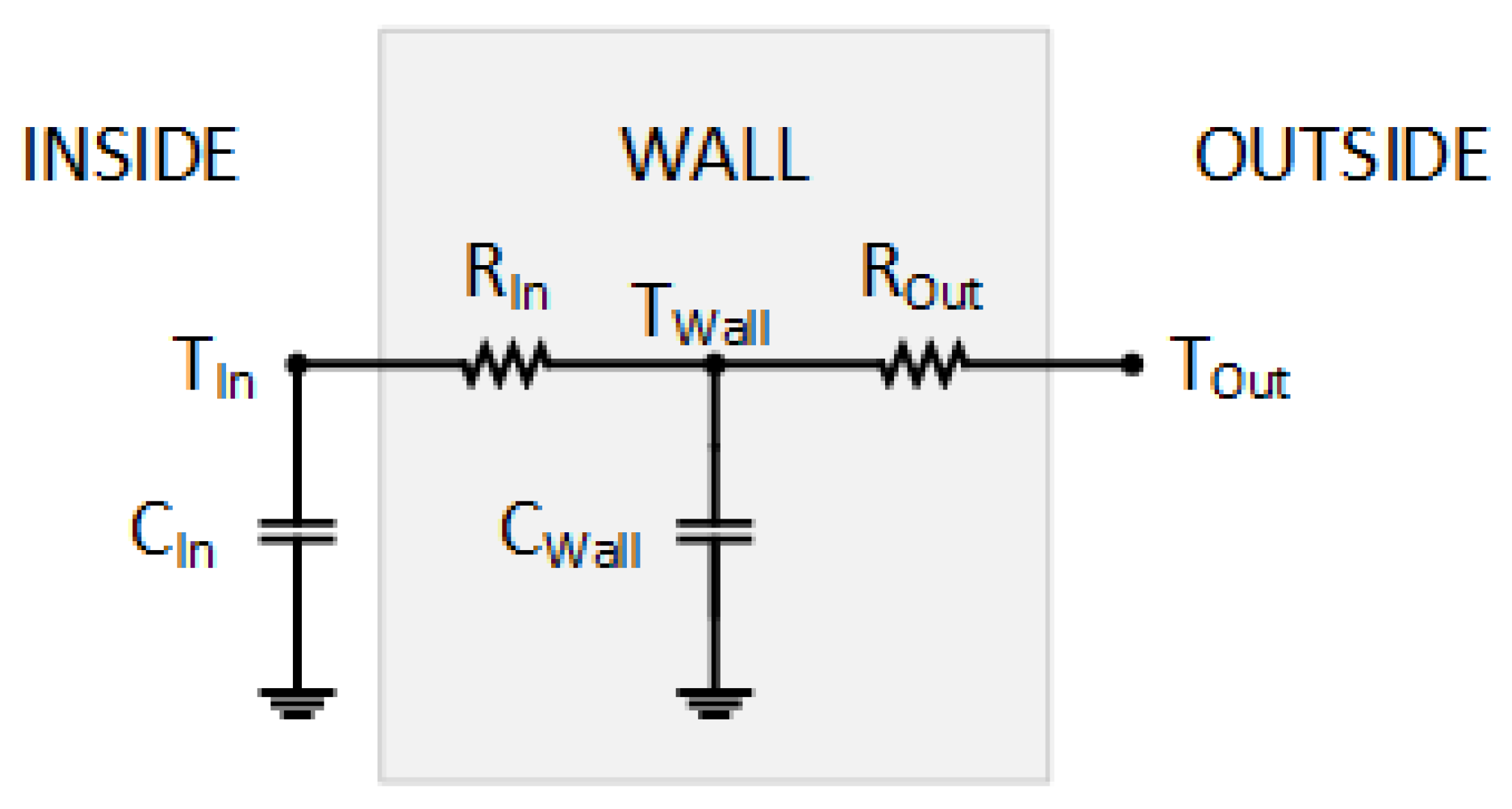
2.1. Example for a Single Wall
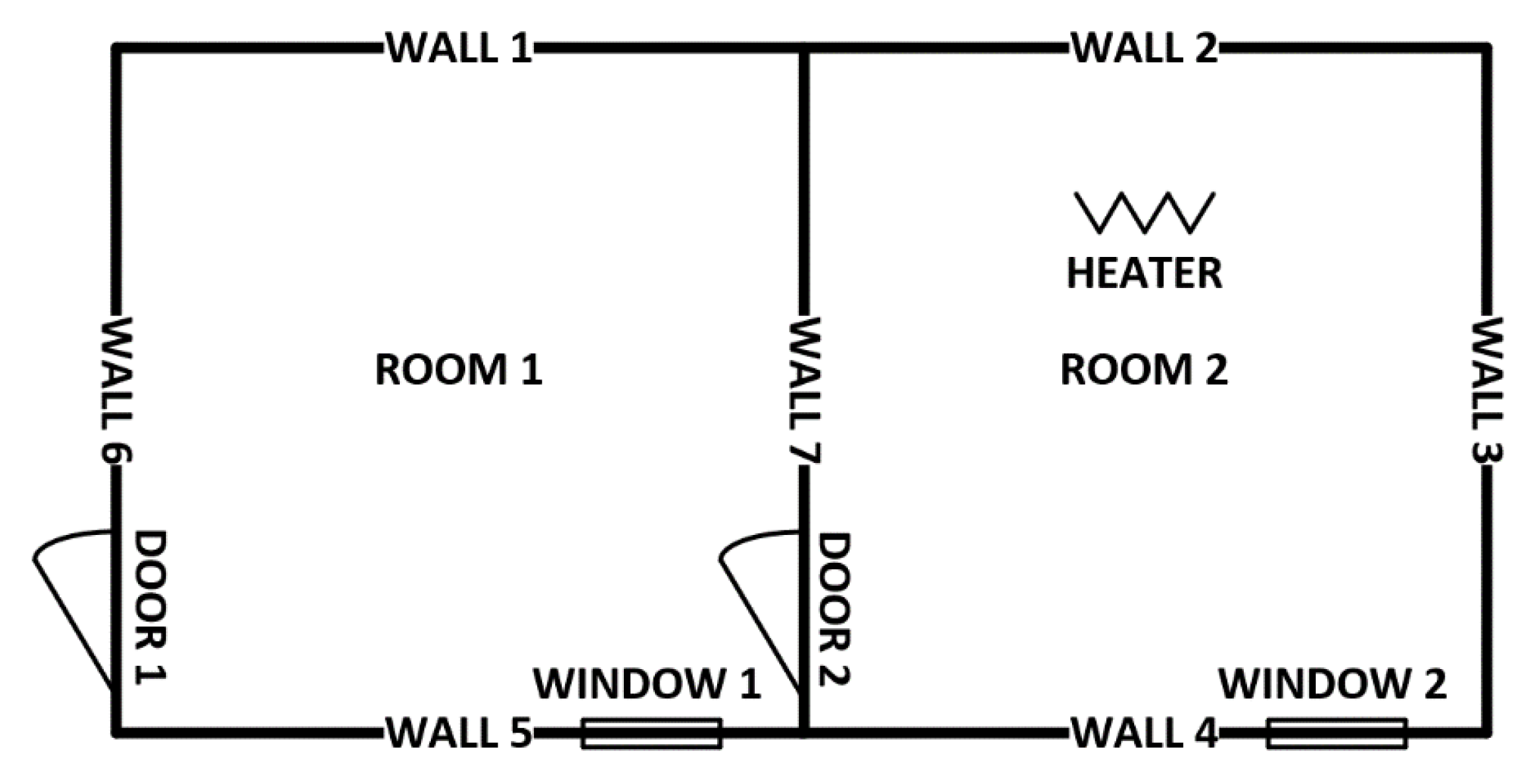
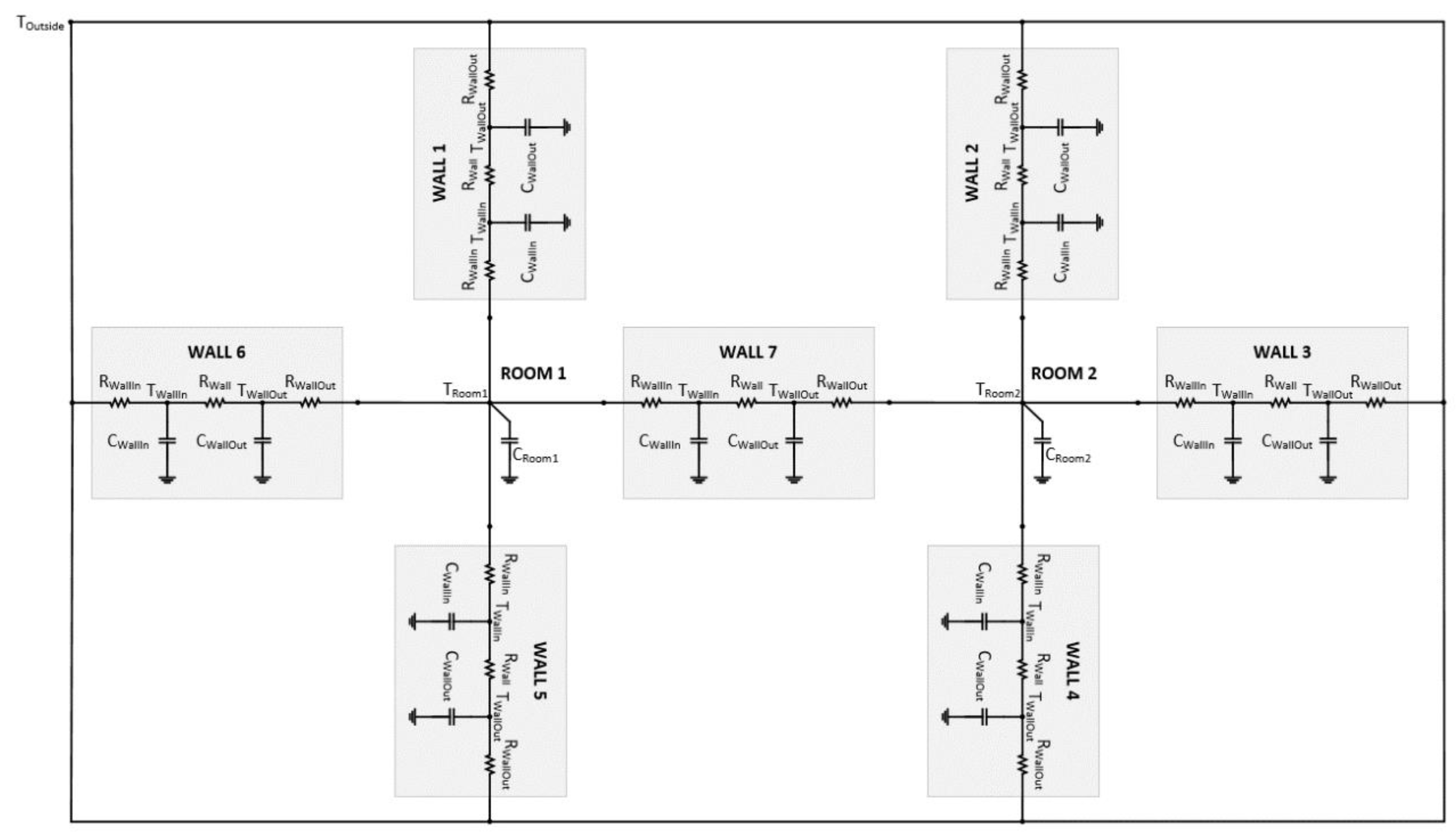
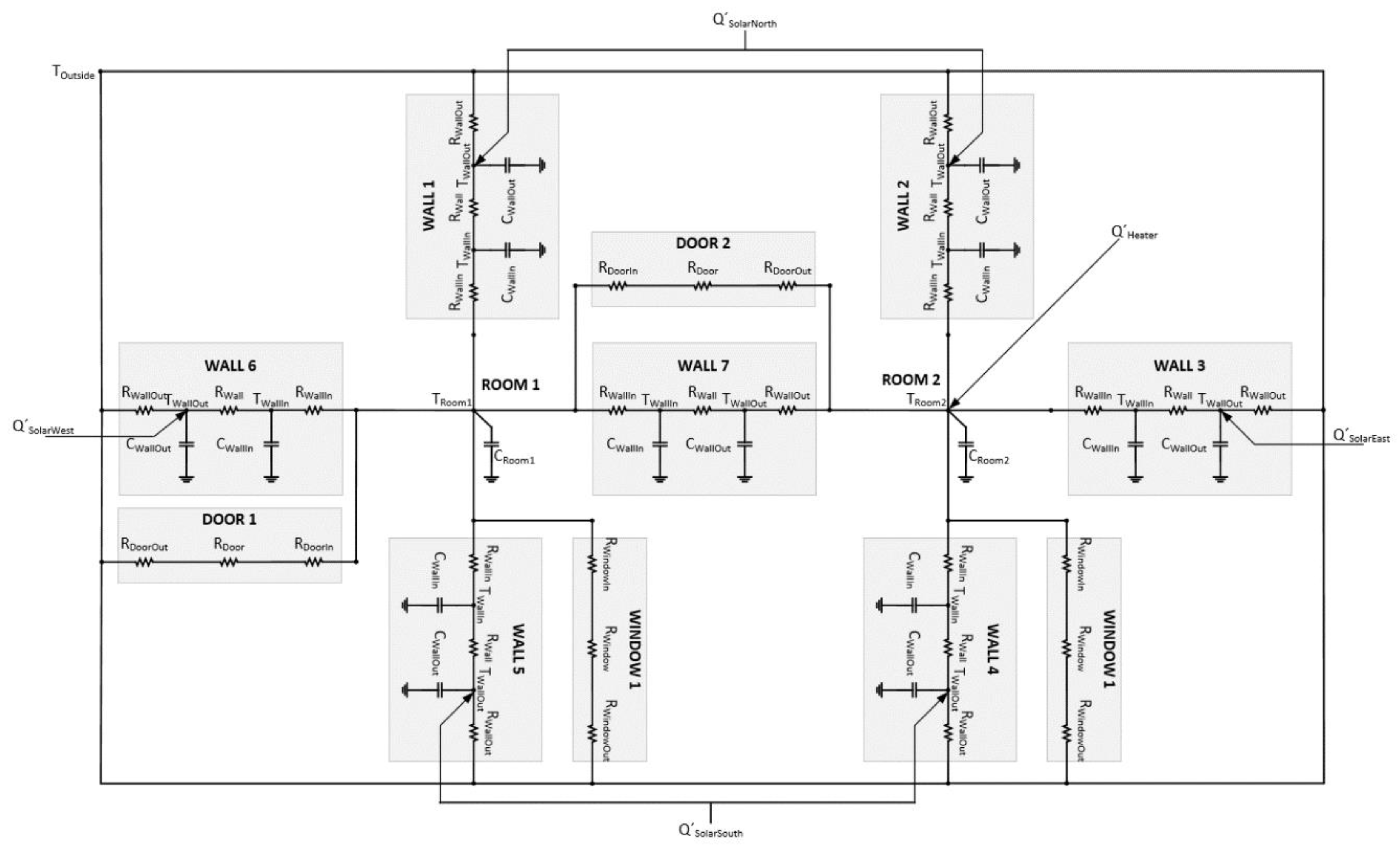
2.2. Example for a Simple Multi-Zone Building
| A= | −2.00 | 1.00 | 0 | 0 | 0 | 0 | 0 | 0 | 0 | 0 | 0 | 0 | 0 | 0 | 0 | 0 |
| 1.00 | −2.00 | 0 | 0 | 0 | 0 | 0 | 0 | 0 | 0 | 0 | 0 | 0 | 0 | 1.00 | 0 | |
| 0 | 0 | −2.00 | 1.00 | 0 | 0 | 0 | 0 | 0 | 0 | 0 | 0 | 0 | 0 | 0 | 0 | |
| 0 | 0 | 1.00 | −2.00 | 0 | 0 | 0 | 0 | 0 | 0 | 0 | 0 | 0 | 0 | 0 | 1.00 | |
| 0 | 0 | 0 | 0 | −2.00 | 1.00 | 0 | 0 | 0 | 0 | 0 | 0 | 0 | 0 | 0 | 1.00 | |
| 0 | 0 | 0 | 0 | 1.00 | −2.00 | 0 | 0 | 0 | 0 | 0 | 0 | 0 | 0 | 0 | 0 | |
| 0 | 0 | 0 | 0 | 0 | 0 | −2.00 | 1.00 | 0 | 0 | 0 | 0 | 0 | 0 | 0 | 1.00 | |
| 0 | 0 | 0 | 0 | 0 | 0 | 1.00 | −2.00 | 0 | 0 | 0 | 0 | 0 | 0 | 0 | 0 | |
| 0 | 0 | 0 | 0 | 0 | 0 | 0 | 0 | −2.00 | 1.00 | 0 | 0 | 0 | 0 | 1.00 | 0 | |
| 0 | 0 | 0 | 0 | 0 | 0 | 0 | 0 | 1.00 | −2.00 | 0 | 0 | 0 | 0 | 0 | 0 | |
| 0 | 0 | 0 | 0 | 0 | 0 | 0 | 0 | 0 | 0 | −2.00 | 1.00 | 0 | 0 | 0 | 0 | |
| 0 | 0 | 0 | 0 | 0 | 0 | 0 | 0 | 0 | 0 | 1.00 | −2.00 | 0 | 0 | 1.00 | 0 | |
| 0 | 0 | 0 | 0 | 0 | 0 | 0 | 0 | 0 | 0 | 0 | 0 | −2.00 | 1.00 | 1.00 | 0 | |
| 0 | 0 | 0 | 0 | 0 | 0 | 0 | 0 | 0 | 0 | 0 | 0 | 1.00 | −2.00 | 0 | 1.00 | |
| 0 | 1.00 | 0 | 0 | 0 | 0 | 0 | 0 | 1.00 | 0 | 0 | 1.00 | 1.00 | 0 | −5.00 | 0.33 | |
| 0 | 0 | 0 | 1.00 | 1.00 | 0 | 1.00 | 0 | 0 | 0 | 0 | 0 | 0 | 1.00 | 0.33 | −4.67 |
| B= | 1.00 | 1.00 | 0 | 0 | 0 | 0 |
| 0 | 0 | 0 | 0 | 0 | 0 | |
| 1.00 | 1.00 | 0 | 0 | 0 | 0 | |
| 0 | 0 | 0 | 0 | 0 | 0 | |
| 0 | 0 | 0 | 0 | 0 | 0 | |
| 1.00 | 0 | 1.00 | 0 | 0 | 0 | |
| 0 | 0 | 0 | 0 | 0 | 0 | |
| 1.00 | 0 | 0 | 1.00 | 0 | 0 | |
| 0 | 0 | 0 | 0 | 0 | 0 | |
| 1.00 | 0 | 0 | 1.00 | 0 | 0 | |
| 1.00 | 0 | 0 | 0 | 1.00 | 0 | |
| 0 | 0 | 0 | 0 | 0 | 0 | |
| 0 | 0 | 0 | 0 | 0 | 0 | |
| 0 | 0 | 0 | 0 | 0 | 0 | |
| 0.67 | 0 | 0 | 0 | 0 | 0 | |
| 0.33 | 0 | 0 | 0 | 0 | 1.00 |
| C= | 0 | 0 | 0 | 0 | 0 | 0 | 0 | 0 | 0 | 0 | 0 | 0 | 0 | 0 | 1.00 | 0 |
| 0 | 0 | 0 | 0 | 0 | 0 | 0 | 0 | 0 | 0 | 0 | 0 | 0 | 0 | 0 | 1.00 |
| D= | 0 | 0 | 0 | 0 | 0 | 0 |
| 0 | 0 | 0 | 0 | 0 | 0 |
2.3. Estimation of Parameters
3. Detailed Modeling of Multi-Zone Buildings with Algorithm and Optimization of Parameters
3.1. The Algorithm for Automatic Definition of the Model Structure Based on the RC Method
- Source I—Represents a heat flow to the system (radiator, the solar radiation, etc.) or input of the system. Its only parameter is type, which states whether this input is a disturbance (e.g., the solar radiation) or a manipulated variable (e.g., the influence of HVAC system).
- Space P—Represents a temperature inside a zone. This is both an output and a state of the system. Its parameters are: Type (required), stating if this is a zone or an outside space (special case in which this temperature is a disturbance); thermal capacity C (required); source (not required), which defines if this space is affected by some (previously defined) source I.
- Wall Z—Represents a wall between two spaces P (either interior or inside; which includes floors and ceilings) and as such adds states to the system (but not outputs). Its parameters are: Spaces P1 and P2 (required), defining which of two (previously defined) spaces is this wall; physical properties (required), or values of R and C parameters (exact number or R and C parameters depends on the desired complexity, e.g., 2R1C or 4R3C, etc.); sources (not required), defining if this wall is affected by some (previously defined) sources I1 and I2 and on which side.
- Opening O—Represents a door or window between spaces (similar to walls). Its parameters are: Spaces (required), defining which of two (previously defined) spaces P1 and P2 is this opening; physical properties (required); or values of R. There are two assumptions: That openings do not have thermal capacity and that they cannot be influenced by heat sources.
| Algorithm 1. The definition of the number of states, inputs and outputs and their vectors and matrices (pseudo-code representation) |
| states_count = length of walls ∗ 2 + length of spaces – 1 inputs_count = length of inputs + 1 outputs_count = lengths of spaces − 1 T = concatenate walls and spaces without outside space u = concatenate outside space and sources y = spaces without outside space A = new empty matrix (states_count × states_count) B = new empty matrix (states_count × inputs_count) C = new empty matrix (outputs_count × states_count) D = new empty matrix (outputs_count × intputs_count) |
| Algorithm 2. The definition of the structure of the state matrix A—walls and spaces (pseudo-code representation) |
| i = 0 for each wall WALL in walls A(i, i) = −1 ∗ ((1/(WALL.R1 ∗ WALL.C1) + (1/(WALL.R ∗ WALL.C1)) A(i, i + 1) = 1/(WALL.R ∗ WALL.C1) A(i + 1, i) = 1/(WALL.R ∗ WALL.C2) A(i + 1, i + 1) = −1 ∗ ((1/(WALL.R ∗ WALL.C2)) + (1/(WALL.R2 ∗ WALL.C2))) j = states_count − outputs_count for each space SPACE is spaces if SPACE is not outside space, then if WALL.P1 = SPACE, then A(i, j) = 1/(WALL.R1 ∗ WALL.C1) A(j, i) = 1/(WALL.R1 ∗ SPACE.C) A(j, j) = A(j, j) − 1/(WALL.R1 ∗ SPACE.C) if WALL.P2 = SPACE, then A(i + 1, j) = 1/(WALL.R2 ∗ WALL.C2) A(j, i + 1) = 1/(WALL.R2 ∗ SPACE.C) A(j, j) = A(j, j) − 1/(WALL.R_2 ∗ SPACE.C) j = j + 1 i = i + 2 |
| Algorithm 3. The modification of the state matrix A—openings and spaces (pseudo-code representation) |
| for each opening OPENING i = states_count − outputs_count for each space P1 in spaces j = states_count − outputs_count for each space P2 in spaces if OPENING.P1 = P1 and OPENING.P2=P2, then if both P1 and P2 are not outside space, then A(i, i) = A(i, i) − 1/((OPENING.R1 + OPENING.R + OPENING.R2) ∗ P1.C) A(i, j) = A(i, j) + 1/((OPENING.R1 + OPENING.R + OPENING.R2) ∗ P1.C) A(j, i) = A(j, i) + 1/((OPENING.R1 + OPENING.R + OPENING.R2) ∗ P2.C) A(j, j) = A(j, j) − 1/((OPENING.R1 + OPENING.R + OPENING.R2) ∗ P2.C) else if P1 is outside space, and P2 is not, then A(j, j) = A(j, j) − 1/((OPENING.R1 + OPENING.R + OPENING.R2) ∗ P2.C) else if P2 is outside space, and P1 is not, then A(i, i) = A(i, i) − 1/((OPENING.R1 + OPENING.R + OPENING.R2) ∗ P1.C) if P2 is not outside space, then j = j + 1 if P1 is not outside space, then i = i + 1 |
| Algorithm 4. The definition of the structure of the input matrix B—walls, spaces and sources (pseudo-code representation) |
| i = 0 for each wall WALL in walls if WALL.P1 is outside space, then B(i, 0) = 1/(WALL.R1 ∗ WALL.C1) if WALL.P2 is outside space, then B(i + 1, 0) = 1/(WALL.R2 ∗ WALL.C2) j = 1 for each source I in sources if I is disturbance if WALL.I1 = In then B(i, j) = 1/(WALL.C1) if WALL.I2 = I, then B(i + 1, j) = 1/(WALL.C2) j = j + 1 for each source I in sources if I is controllable, then if WALL.I1 = I, then B(i, j) = 1/(WALL.C1) if WALL.I2 = I, then B(i + 1, j) = 1/(WALL.C2) j = j + 1 i = i + 2 |
| Algorithm 5. The modification of the input matrix B—openings and spaces (pseudo-code representation) |
| for each opening OPENING in openings i = states_count − outputs_count for each space P1 in spaces j = states_count − outputs_count for each space P2 in spaces if OPENING.P1 = P1 and OPENING.P2=P2, then if P1 is outside space and P2 is not, then B(j, 0) = B(j, 0) + 1/((OPENING.R1 + OPENING.R + OPENING.R2) ∗ P2.C) else if P2 is outside space and P1 is not, then B(i, 0) = B(i, 0) + 1/((OPENING.R1 + OPENING.R + OPENING.R2) ∗ P1.C) if P2 is not outside space, then j = j + 1 if P1 is not outside space, then i = i + 1 |
| Algorithm 6. The modification of the input matrix B—spaces and sources (pseudo-code representation) |
| i = states_count − outputs_count for each space SPACE in spaces j = 1 for each source I in sources if I is disturbance, then if SPACE.I = I, then B(i, j) = 1/SPACE.C j = j + 1 for each source I in sources if I is controllable, then if SPACE.I = I, then B(i, j) = 1/SPACE.C j = j + 1 if SPACE is outside space, then i = i + 1 |
| Algorithm 7. The definition of structure of the output matrix C (pseudo-code representation) |
| i = 0 k = states_count − outputs_count for each space SPACE in spaces if SPACE is not outside space, then C(i, k) = 1 i = k + 1 k = k + 1 |
3.2. Optimization of the Model Parameters Based on the Measured Data
- missing technical data about the building (lost documentation or documentation being not detailed enough),
- suspicion about correctness of information (did the constructor really build according to the technical documentation),
- parameter or properties that are unknown or hard to measure (for example, the heat transfer coefficient that depends on the speed of wind),
- ageing of materials and structures, etc.
- Selection of the solver and the algorithm for optimization problem: fminsearch (Simplex/Derivative-Free), fminunc (Quasi-Newton), fmincon (Interior-Point, SQP, Active-Set), lsqnonlin (Levenberg–Marquardt algorithm) [37];
- Selection of the optimization criterion: Total error, root-mean-square error, normalized RMS error, maximum error;
- Sampling period: 900 s (15 min) and 3600 s (1 h).
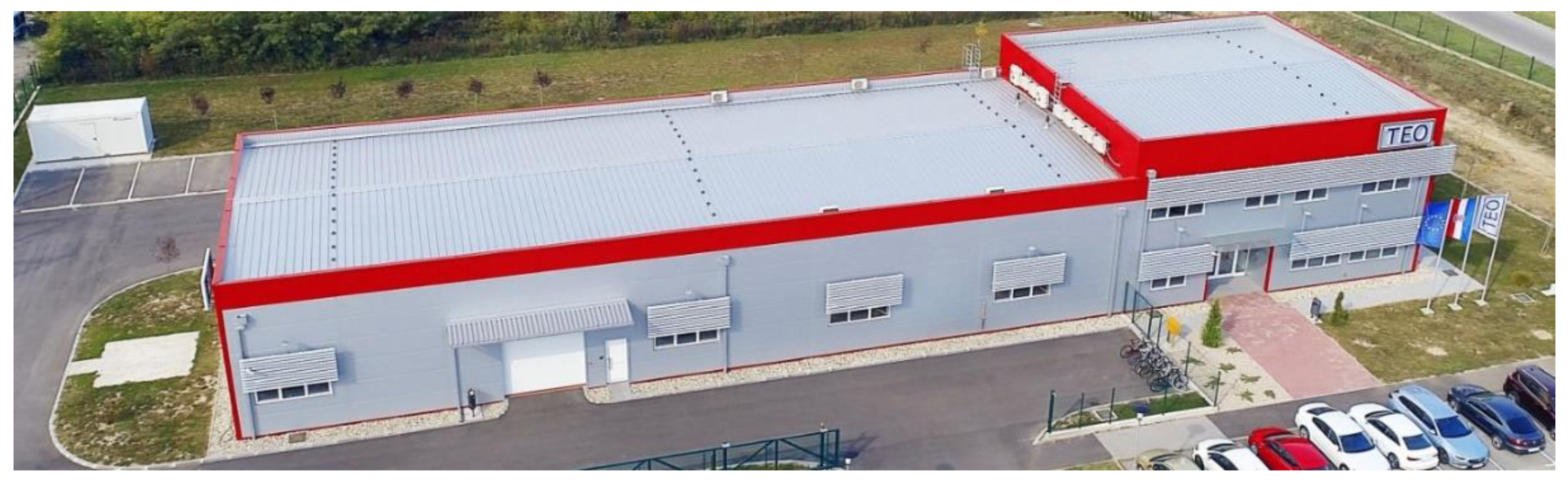
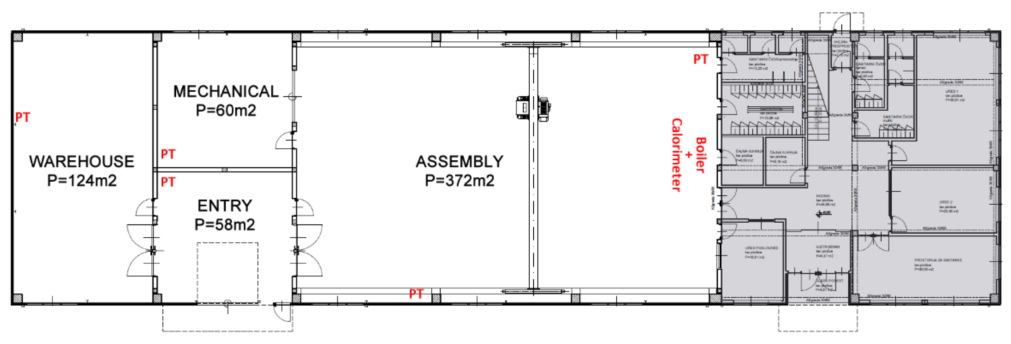
4. Case Study
4.1. Building, HVAC System, Measurement
- a temperature sensor in each zone (the assembly has two sensors, but an average was used),
- a calorimeter for measuring the heat flow from the boiler (two temperature sensors on pipes and flow sensor),
- a weather station on the outside, capable of measuring the outside temperature and the solar radiation (among other measurements).
4.2. Initial Model of Building End Estimation of Parameters
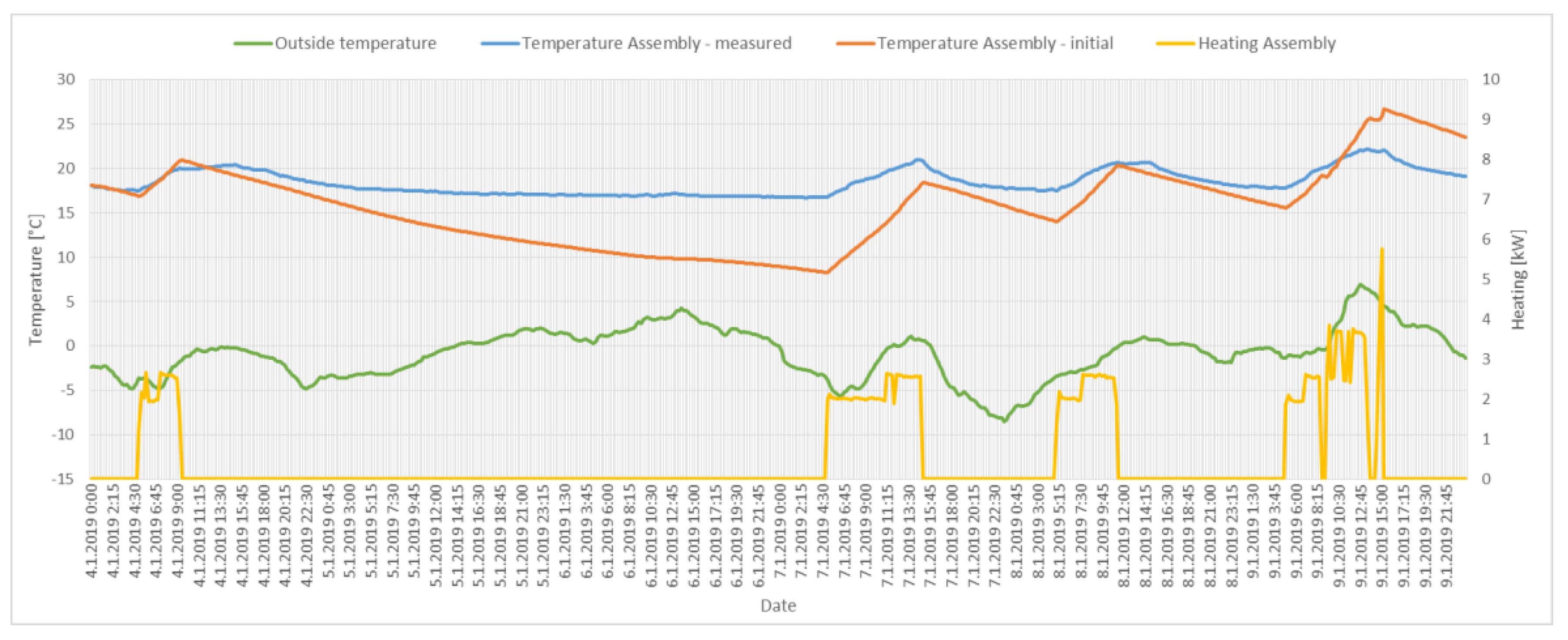
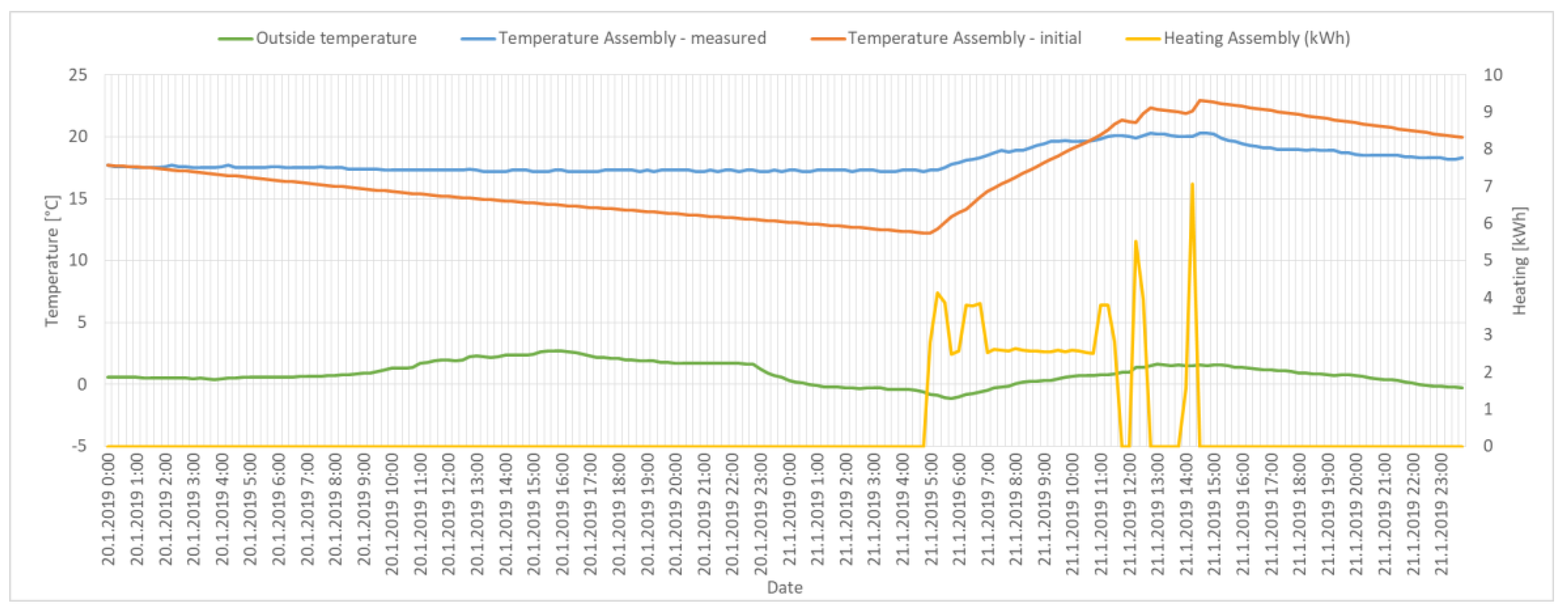
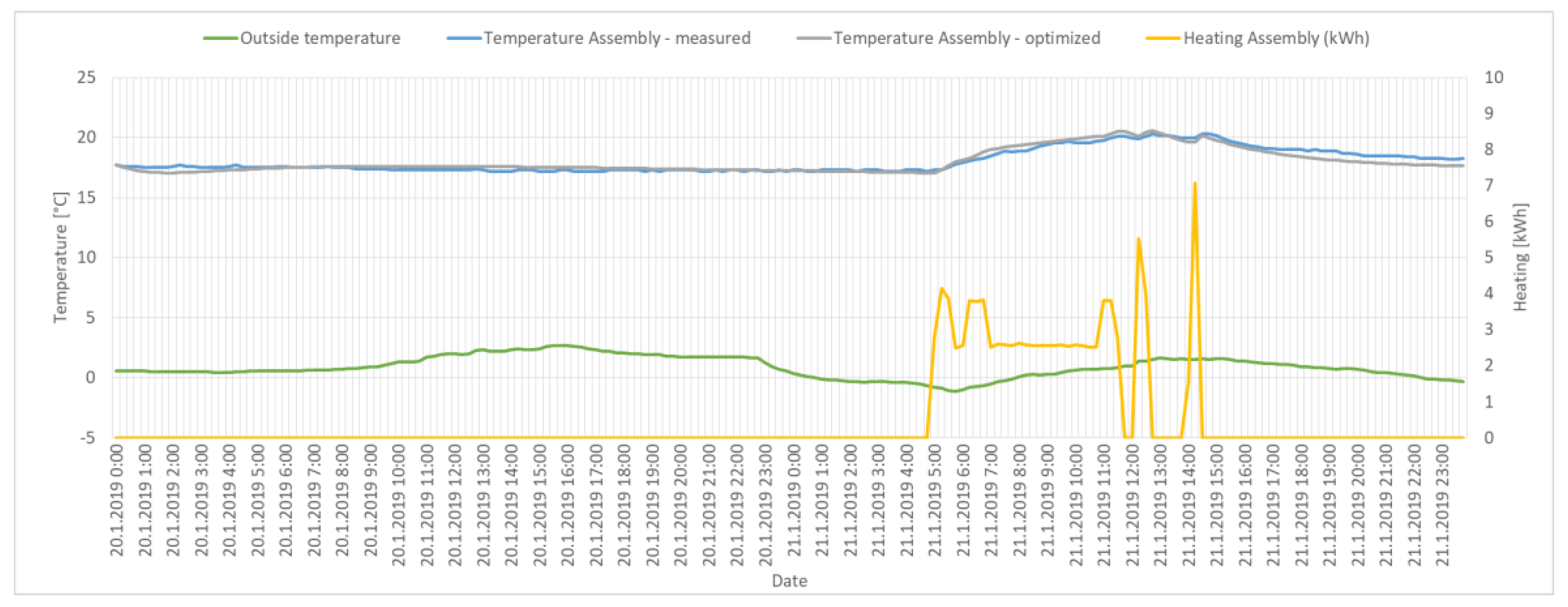
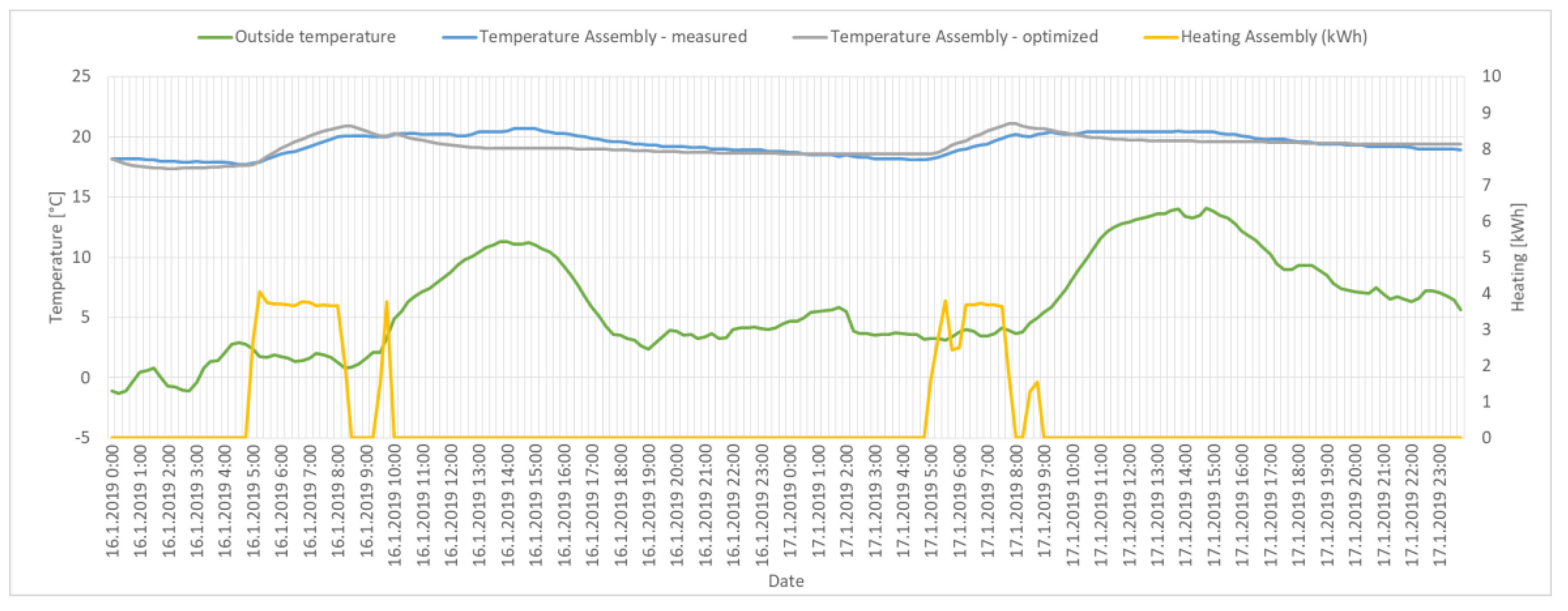
4.3. Results
5. Conclusions
Author Contributions
Funding
Data Availability Statement
Conflicts of Interest
Nomenclature
| General abbreviations | ||
| RC | Resistive-Capacitive | |
| MPC | Model Predictiove Control | |
| HVAC | Heating, Ventilation, Air-Conditioning | |
| 2R1C | 2 Resistances and 1 Capacity | |
| 3R2C | 3 Resistances and 2 Capacity | |
| 4R3C | 4 Resistances and 3 Capacity | |
| R | Equivalent thermal resistance | |
| C | Equivalent thermal capacity | |
| Example for a single wall | ||
| TIn | Temperature of the inside space (room) | °C |
| TOut | Temperature of the outside space | °C |
| ROut | Thermal resistance between the wall and the outside space | K/W |
| RIn | Thermal resistance between the wall and the inside (room) | K/W |
| CWall | Thermal capacity of the wall | J/K |
| TWall | Internal temperature of the wall | °C |
| CIn | Thermal capacity of air and element of the inside space (room) | J/K |
| Example for a simple multi-zone building | ||
| TOutside | Temperature of the outside space | °C |
| TRoom1 | Temperature inside room 1 | °C |
| TRoom2 | Temperature inside room 2 | °C |
| CRoom1 | Thermal capacity of air and element inside room 1 | J/K |
| CRoom2 | Thermal capacity of air and element inside room 2 | J/K |
| TWallIn | Temperature on the surface of the wall on the inside (considering reference zone/room) | °C |
| TWallOut | Temperature on the surface of the wall on the outside (considering reference zone/room) | °C |
| RWallIn | Thermal resistance of the wall and the inside (considering reference zone/room)—convection | K/W |
| RWall | Thermal resistance inside the wall—conduction | K/W |
| RWallOut | Thermal resistance of the wall and the outside (considering reference zone/room)—convection | K/W |
| CWallIn | Thermal capacity of the inside part of the wall (considering reference zone/room) | J/K |
| CWallOut | Thermal capacity of the outside part of the wall (considering reference zone/room) | J/K |
| RWindowIn | Thermal resistance of the windows and the inside (considering reference zone/room)—convection | K/W |
| RWindow | Thermal resistance inside the windows—conduction | K/W |
| RWindowOut | Thermal resistance of the windows and the outside (considering reference zone/room)—convection | K/W |
| QHeater | Heat from the heater | J |
| QSolarNorth | Heat by solar radiation (north component) | J |
| QSolarEast | Heat by solar radiation (east component) | J |
| QSolarSouth | Heat by solar radiation (south component) | J |
| QSolarWest | Heat by solar radiation (west component) | J |
| Heat flow | W | |
| State-space representation | ||
| A | System matrix | |
| B | Input matrix | |
| C | Output matrix | |
| D | Feed-forward matrix | |
| T | State vectors (temperatures) | |
| u | Input vector | |
| y | Output vector | |
| ai,j | Element of system matrix A in i-th column and j-th row | |
| bi,j | Element of input matrix B in i-th column and j-th row | |
| ci,j | Element of output matrix C in i-th column and j-th row | |
| di,j | Element of feed-forward matrix D in i-th column and j-th row | |
| Estimation of parameters | ||
| Heat flow | W | |
| h | Heat transfer coefficient | W/m2K |
| A | Surface of the wall | m2 |
| ΔT | Difference in temperature (e.g., between wall and surrounding fluid) | K |
| RConv | Thermal resistance of convection | K/W |
| k | Coefficient of thermal conductivity | W/mK |
| l | Thickness of the wall | M |
| RCond | Thermal resistance of conduction | K/W |
| Radiation thermal conductance | W/m2K | |
| RRad | Thermal resistance of radiation | K/W |
| C | Thermal capacity | J/K |
| c | Specific heat capacity | J kg/K |
| ρ | Density | kg/m3 |
| V | Volume | m3 |
| Algorithm for automatic definition of model structure based on RC method | ||
| I (Source) | Object representing a source (heat flow) | |
| P (Space) | Object representing a space (zone, room) | |
| P.C | Parameter of object Space with value of its thermal capacity | |
| P.I | Parameter of object Space, pointer to object Source that is affecting this space | |
| Z (Wall) | Object representing a wall (vertical wall, floor, ceiling) | |
| Z.P | Parameter of object Wall, pointer to object Space that is adjacent to this wall (always two such parameters) | |
| Z.R | Parameter of object Wall with value of its thermal resistance (one or more, ordered as points to adjacent Spaces) | |
| Z.C | Parameter of object Wall with value of its thermal capacity (one or more, ordered as points to adjacent Spaces) | |
| Z.I | Parameter of object space, pointer to object Source that is affecting this space (always two, ordered as points to adjacent Spaces) | |
| O (Opening) | Object representing an opening (door, window) | |
| O.P | Parameter of object Opening, pointer to object Space that is adjacent to this wall (always two such parameters) | |
| O.R | Parameter of object Opening with value of its thermal resistance (one or more, ordered as points to adjacent Spaces) | |
| sources | Ordered indexed list with all sources (objects I) | |
| spaces | Ordered indexed list with all spaces (objects P) | |
| walls | Ordered indexed list with all walls (objects Z) | |
| openings | Ordered indexed list with all sources (objects O) | |
| states | Vector with states (of the system) | |
| inputs | Vector with inputs (to the system) | |
| outputs | Vector with outputs (from the system) | |
| i, j, k | Indexes | |
| Optimization of model parameters based on measured data | ||
| AR | State matrix of the referent model | |
| BR | Input matrix of the referent model | |
| fR(AR,BR) | Function representing the referent model, defined by its state and input matrix | |
| yR | Outputs of the referent model | |
| u | Inputs to the model | |
| AT | State matrix of the testing model | |
| BT | Input matrix of the testing model | |
| fT(AT,BT) | Function representing the testing model, defined by its state and input matrix | |
| yT | Outputs of the testing model | |
| RMSE | Root-Mean-Square Error | |
| Q | Number of outputs | |
| K | Number of measurements in time series | |
| Output of the referent model, where i is index of output in output vector and j is index of output in time series | ||
| Output of the referent model, where i is index of output in output vector and j is index of output in time series | ||
| MaxErr | Maximum Error | |
Appendix A

| Construction Element | Property | Unit | Value |
|---|---|---|---|
| Walls side 1 outer layer | heat transfer coefficient | W/m2K | 0.0975 |
| Walls inner layer | width | m | 0.2 |
| Walls inner layer | specific heat capacity | J/kgK | 1 |
| Walls side 2 outer layer | heat transfer coefficient | W/m2K | 0.0975 |
| Spaces | density | kg/m2 | 1.205 |
| Spaces | specific heat capacity | J/kgK | 1010 |
| Openings side 1 outer layer | width | m | 0.005 |
| Openings side 1 outer layer | heat transfer coefficient | W/m2K | 1.05 |
| Openings inner layer | width | m | 0.005 |
| Openings inner layer | heat transfer coefficient | W/m2K | 0.001772 |
| Openings side 2 outer layer | width | m | 0.005 |
| Openings side 2 outer layer | heat transfer coefficient | W/m2K | 1.05 |
References
- Vakiloroaya, V.; Samali, B.; Fakhar, A.; Pishghadam, K. A review of different strategies for HVAC energy saving. Energy Convers. Manag. 2014, 77, 738–754. [Google Scholar] [CrossRef]
- Kelso, J.D. Building Energy Data Book 2011; U.S. Department of Energy: Washington, DC, USA, 2012.
- Han, K.; Zhang, J. Energy-saving building system integration with a smart and low-cost sensing/control network for sustainable and healthy living environments: Demonstration case study. Energy Build. 2020, 214, 109861. [Google Scholar] [CrossRef]
- Han, J.; Lee, E.; Cho, H.; Yoon, Y.; Lee, H.; Rhee, W. Improving the Energy Saving Process with High-Resolution Data: A Case Study in a University Building. Sensors 2018, 18, 1606. [Google Scholar] [CrossRef] [PubMed] [Green Version]
- Huang, Q. Occupancy-Driven Energy-Efficient Buildings Using Audio Processing with Background Sound Cancellation. Buildings 2018, 8, 78. [Google Scholar] [CrossRef] [Green Version]
- Purdon, S.; Kusy, B.; Jurdak, R.; Challen, G. Model-free HVAC control using occupant feedback. In Proceedings of the 38th Annual IEEE Conference on Local Computer Networks—Workshops, Sydney, NSW, Australia, 21–24 October 2013; pp. 84–92. [Google Scholar]
- Ma, Y.; Kelman, A.; Daly, A.; Borrelli, F.; Yudong, M. Predictive Control for Energy Efficient Buildings with Thermal Storage. IEEE Control Syst. Mag. 2012, 32, 44–64. [Google Scholar]
- Fraisse, G.; Viardot, C.; Lafabrie, O.; Achard, G. Development of a simplified and accurate building model based on electrical analogy. Energy Build. 2002, 34, 1017–1031. [Google Scholar] [CrossRef]
- Atam, E.; Helsen, L. Control-Oriented Thermal Modeling of Multizone Buildings: Methods and Issues: Intelligent Control of a Building System. IEEE Control Syst. 2016, 36, 86–111. [Google Scholar]
- Fayazbakhsh, M.A.; Bagheri, F.; Bahrami, M. A Resistance–Capacitance Model for Real-Time Calculation of Cooling Load in HVAC-R Systems. J. Therm. Sci. Eng. Appl. 2015, 7, 1–9. [Google Scholar] [CrossRef]
- Goyal, S.; Liao, C.; Barooah, P. Identification of multi-zone building thermal interaction model from data. In Proceedings of the IEEE Conference on Decision and Control and European Control Conference, Orlando, FL, USA, 12–15 December 2011; pp. 181–186. [Google Scholar]
- Neill, Z.O.; Narayanan, S.; Brahme, R.; O’Neill, Z.; Narayanan, S.; Brahme, R. Model-based thermal load estimation in buildings. In Proceedings of the Fourth National Conference of IBPSA-USA, New York, NY, USA, 11–13 August 2010; pp. 474–481. [Google Scholar]
- Bengea, S.; Adetola, V.; Kang, K.; Liba, M.J.; Vrabie, D.; Bitmead, R.; Narayanan, S. Parameter estimation of a building system model and impact of estimation error on closed-loop performance. In Proceedings of the IEEE Conference on Decision and Control and European Control Conference, Orlando, FL, USA, 12–15 December 2011; pp. 5137–5143. [Google Scholar]
- Bagheri, A.; Genikomsakis, K.N.; Feldheim, V.; Ioakimidis, C.S. Sensitivity Analysis of 4R3C Model Parameters with Respect to Structure and Geometric Characteristics of Buildings. Energies 2021, 14, 657. [Google Scholar] [CrossRef]
- Ma, Y.; Anderson, G.; Borrelli, F. A Distributed Predictive Control Approach to Building Temperature Regulation. In Proceedings of the American Control Conference, San Francisco, CA, USA, 29 June–1 July 2011; pp. 2089–2094. [Google Scholar]
- Bacher, P.; Madsen, H. Identifying suitable models for the heat dynamics of buildings. Energy Build. 2011, 43, 1511–1522. [Google Scholar] [CrossRef] [Green Version]
- Harb, H.; Boyanov, N.; Hernandez, L.; Streblow, R.; Müller, D. Development and validation of grey-box models for forecasting the thermal response of occupied buildings. Energy Build. 2016, 117, 199–207. [Google Scholar] [CrossRef]
- Lee, K.; Braun, J.E. Development and Application of an Inverse Building Model for Demand Response in Small Commercial Buildings. In Proceedings of the SimBuild 2004, IBPSA-USA National Conference, Boulder, CO, USA, 4–6 August 2004; pp. 1–12. [Google Scholar]
- Ogunsola, O.T.; Song, L.; Wang, G. Development and validation of a time-series model for real-time thermal load estimation. Energy Build. 2014, 76, 440–449. [Google Scholar] [CrossRef]
- Lin, Y.; Middelkoop, T.; Barooah, P. Issues in identification of control-oriented thermal models of zones in multi-zone buildings. In Proceedings of the 2012 IEEE 51st IEEE Conference on Decision and Control (CDC), Maui, HI, USA, 10–13 December 2012; pp. 6932–6937. [Google Scholar]
- Li, Y.; Castiglione, J.; Astroza, R.; Chen, Y. Real-time thermal dynamic analysis of a house using RC models and joint state-parameter estimation. Build. Environ. 2021, 188, 107184. [Google Scholar] [CrossRef]
- Boodi, A.; Beddiar, K.; Amirat, Y.; Benbouzid, M. Simplified Building Thermal Model Development and Parameters Evaluation Using a Stochastic Approach. Energies 2020, 13, 2899. [Google Scholar] [CrossRef]
- Prívara, S.; Váňa, Z.; Gyalistras, D.; Cigler, J.; Sagerschnig, C.; Morari, M.; Ferkl, L. Modeling and identification of a large multi-zone office building. In Proceedings of the 2011 IEEE International Conference on Control Applications (CCA), Denver, CO, USA, 28–30 September 2011; pp. 55–60. [Google Scholar]
- Belic, F.; Hocenski, Z.; Sliskovic, D. Algorithm for defining structure of thermal model of building based on RC analogy. In Proceedings of the 2019 23rd International Conference on System Theory, Control and Computing (ICSTCC), Sinaia, Romania, 9–11 October 2019; pp. 580–585. [Google Scholar]
- Brastein, O.M.; Perera, D.W.U.; Pfeifer, C.; Skeie, N.-O. Parameter estimation for grey-box models of building thermal behaviour. Energy Build. 2018, 169, 58–68. [Google Scholar] [CrossRef] [Green Version]
- Gerlich, V. Modelling Of Heat Transfer in Buildings. In ECMS 2011 Proceedings; Burczynski, T., Kolodziej, J., Byrski, A., Carvalho, M., Eds.; ECMS: Koblenz, Germany, 2011; pp. 244–248. [Google Scholar]
- Underwood, C.P.; Yik, F.W.H. Modelling Methods for Energy in Buildings; Blackwell Publishing Ltd.: Oxford, UK, 2004. [Google Scholar]
- Deng, K.; Barooah, P.; Mehta, P.G.; Meyn, S.P. Building Thermal Model Reduction via Aggregation of States. In Proceedings of the American Control Conference (ACC), Baltimore, MD, USA, 30 June–2 July 2010; pp. 5118–5123. [Google Scholar]
- Wang, S.; Xu, X. Parameter estimation of internal thermal mass of building dynamic models using genetic algorithm. Energy Convers. Manag. 2006, 47, 1927–1941. [Google Scholar] [CrossRef]
- Wang, Z.; Chen, Y.; Li, Y. Development of RC model for thermal dynamic analysis of buildings through model structure simplification. Energy Build. 2019, 195, 51–67. [Google Scholar] [CrossRef]
- Negenborn, R.R.; Maestre, J.M. Distributed Model Predictive Control: An Overview and Roadmap of Future Research Opportunities. IEEE Control Syst. 2014, 34, 87–97. [Google Scholar]
- Bejan, A.; Kraus, A.D. Heat Transfer Handbook; John Wiley & Sons: Hoboken, NJ, USA, 2003. [Google Scholar]
- Davies, M.G. Building Heat Transfer, 1st ed.; John Wiley & Sons: Hoboken, NJ, USA, 2004. [Google Scholar]
- Janna, W.S. Engineering Heat Transfer, 2nd ed.; CRC Press: Memphis, TN, USA, 1999. [Google Scholar]
- Belic, F. ModelBuilder—Application for Creating Thermal Models of Buildings. 2016. Available online: http://dx.doi.org/10.13140/RG.2.1.2027.5605 (accessed on 1 January 2017).
- Belic, F.; Hocenski, Z.; Sliskovic, D. Thermal modeling of buildings with RC method and parameter estimation. In Proceedings of the 2016 International Conference on Smart Systems and Technologies (SST), Osijek, Croatia, 12–14 October 2016; pp. 19–25. [Google Scholar]
- MathWorks. MATLAB Documentation. 2017. Available online: https://www.mathworks.com/help/index.html (accessed on 1 January 2017).
- Belić, F. Hibridna Metoda za Izradu Termodinamičkog Modela Zgrade Temeljena na Otporničko-Kapacitivnoj Analogiji; Josip Juraj Strossmayer University of Osijek: Osijek, Croatia, 2019. [Google Scholar]
- Belic, F. Measurement of Temperatures, HVAC System Values and Weather-Station Readings for Single-Floor Industrial Building in Croatia. Mendeley Data. 2021. Available online: http://dx.doi.org/10.17632/ykjrmrtcxz.1 (accessed on 21 October 2021).


| Step | Action |
|---|---|
| 1. | Definition of the number of states, inputs and outputs and their vectors (T, u and y) and matrices (A, B, C and D) |
| 2. | Definition of the structure and nominal values of elements of the state matrix A from relationships between walls Z and spaces P |
| 3. | Modification of the nominal values of elements of the state matrix A from relationships between openings O and spaces P |
| 4. | Definition of the structure and nominal values of elements of the input matrix B from relationships between walls Z, spaces P and sources I |
| 5. | Modification of the nominal values of elements of the input matrix B from relationships between openings O and spaces P |
| 6. | Modification of the nominal values of elements of the input matrix B from relationships between spaces P and sources I |
| 7. | Definition of the structure and values of elements of the output matrix C (passing values of temperatures of spaces) and the feed-forward matrix D (always a null matrix) |
| a1,1 | a1,2 | a2,1 | a2,2 | |
|---|---|---|---|---|
| Initial values | −1.22 × 10¹⁰ | 1.21 × 10¹⁰ | 1.21 × 10¹⁰ | −1.22 × 10¹⁰ |
| Optimized values | −0.425 | 0.425 | 0.425 | −0.425 |
Publisher’s Note: MDPI stays neutral with regard to jurisdictional claims in published maps and institutional affiliations. |
© 2021 by the authors. Licensee MDPI, Basel, Switzerland. This article is an open access article distributed under the terms and conditions of the Creative Commons Attribution (CC BY) license (https://creativecommons.org/licenses/by/4.0/).
Share and Cite
Belić, F.; Slišković, D.; Hocenski, Ž. Detailed Thermodynamic Modeling of Multi-Zone Buildings with Resistive-Capacitive Method. Energies 2021, 14, 7051. https://doi.org/10.3390/en14217051
Belić F, Slišković D, Hocenski Ž. Detailed Thermodynamic Modeling of Multi-Zone Buildings with Resistive-Capacitive Method. Energies. 2021; 14(21):7051. https://doi.org/10.3390/en14217051
Chicago/Turabian StyleBelić, Filip, Dražen Slišković, and Željko Hocenski. 2021. "Detailed Thermodynamic Modeling of Multi-Zone Buildings with Resistive-Capacitive Method" Energies 14, no. 21: 7051. https://doi.org/10.3390/en14217051
APA StyleBelić, F., Slišković, D., & Hocenski, Ž. (2021). Detailed Thermodynamic Modeling of Multi-Zone Buildings with Resistive-Capacitive Method. Energies, 14(21), 7051. https://doi.org/10.3390/en14217051