OPF of Modern Power Systems Comprising Renewable Energy Sources Using Improved CHGS Optimization Algorithm

Abstract

This article introduces an application of the recently developed hunger games search (HGS) optimization algorithm. The HGS is combined with chaotic maps to propose a new Chaotic Hunger Games search (CHGS). It is applied to solve the optimal power flow (OPF) problem. The OPF is solved to minimize the generation costs while satisfying the systems’ constraints. Moreover, the article presents optimal siting for mixed renewable energy sources, photovoltaics, and wind farms. Furthermore, the effect of adding renewable energy sources on the overall generation costs value is investigated. The exploration field of the optimization problem is the active output power of each generator in each studied system. The CHGS also obtains the best candidate design variables, which corresponds to the minimum possible cost function value. The robustness of the introduced CHGS algorithm is verified by performing the simulation 20 independent times for two standard IEEE systems—IEEE 57-bus and 118-bus systems. The results obtained are presented and analyzed. The CHGS-based OPF was found to be competitive and superior to other optimization algorithms applied to solve the same optimization problem in the literature. The contribution of this article is to test the improvement done to the proposed method when applied to the OPF problem, as well as the study of the addition of renewable energy sources on the introduced objective function.

1. Introduction

In the broadest sense, the scope of electrical power systems is significantly attracting the interest of many researchers all over the world, as the electrical power system is a complicated and dynamic one. The electric power system is considered as an umbrella that covers many subsystems, such as the generation sector, transmission system, and distribution networks [1]. According to the fact that the power system is a complex one, there are many constraints on such electrical power systems. The common constraints are the bus voltage limits, transmission line thermal limit, generator output active and reactive power constraints, etc. [2]. Initially, in solving the well-known economic dispatch (ED) problem, limits of the network itself are overlooked, and only the limits of the generator active power are considered [3,4]. Afterwards, the optimal power flow (OPF) problem is solved to better describe the electrical power system considering the network physical constraints [5]. The OPF problem can be solved for different targets and objectives, such as losses, emission rate, or generation cost minimization [6]. When solving the OPF problem, different network parameters can be set as design variables, such as the generator power and voltage, the transformer tap settings, the reactive power compensators, and others. In the past, traditional optimization methods were used to solve the OPF problem [7,8,9]. Quadratic programming [10], interior point method [11], and more are examples of these traditional methods. These traditional methods suffer from weak points, such as consuming too much time to solve the problem, the possibility of missing the convergence, and the dependency on the initial conditions [12]. Moreover, some mathematical assumptions need to be set for the simplification of the problem. Accordingly, other types of optimization methods are needed to avoid the weaknesses of the traditional optimization methods.

In the literature, different metaheuristic-based optimization methods were used to solve the OPF problem. Advantageously, the metaheuristic-based optimization methods avoided the weak points of the traditional optimization methods [13]. The metaheuristic optimization algorithms are inspired by nature and simulate natural phenomena to reach the best solution after initializing random agents, and then updating them throughout the iterations. For instance, [14] provided modified versions of the genetic algorithm (GA) and discussed their advantages and disadvantages. The new advances in GA were also introduced. Piotrowski in [15] discussed the possibility of using particle swarm optimization (PSO) to solve the problem, which is a well-known population-based metaheuristic optimization method. The problem is to set the PSO population size in detail, according to tests conducted on eight PSO variants. Many benchmarks and applications are used for verification of the problem introduced in this reference. PSO is applied to different scientific scopes, especially in engineering fields and physics. Since being introduced, PSO has been continuously inspected, and this has resulted in the appearance of many modified PSO versions. Tree seed algorithm (TSA) [16] is one of the metaheuristic optimization methods that is inspired by the relationship between the trees and seeds. The trees are generated randomly in the search space. The fitness values of the trees are calculated based on the objective function. After the production of the seeds for a tree, the best seeds are selected. If the fitness of the seed is better than that of that tree, it will replace it. The sine-cosine algorithm (SCA) [17] simulates waveforms of the sine function and the cosine function. The SCA mimics the mathematical formulation of the ‘sine’ and ‘cosine’ functions. The SCA is applied widely for its feature selection besides the update process. Salp swarm algorithm (SSA) [18] is a swarm optimization method that simulates the behavior of the salps. Salps look like jellyfish in movements. This algorithm simulates the salp chain in the deep-sea searching for food. It is known for its high processing, and its few parameters to be adjusted. Hussien et al. introduced sunflower optimization (SFO), and cuttlefish optimization (CFO) algorithms in [19,20,21]. In general, each metaheuristic-based optimization algorithms have their pros and cons [22].

In this article, a newly developed chaotic hunger games search (CHGS) optimization algorithm is introduced as an application of the optimization methods for solving a problem in the electrical power engineering field. The CHGS comes from a combination of the hunger games search (HGS) algorithm [23], with the chaotic maps introduced in [24], of which the effect appears in the initial population. The growing development of soft computation capabilities motivated the researchers for using such an optimization algorithm to solve problems in different fields, and especially, in the field of electrical power engineering problems. The HGS algorithm itself is inspired by the hunger-driven activities of the animals. This optimization method simulates the effect of hunger on the exploration procedures of the animals by designing adaptive weights based on the hunger concept. The optimization process by the introduced CHGS algorithm reached the optimal solution professionally. The process does not get stuck in a local point, but it reaches the global one. The advantage of the CHGS optimization method is its fast and smooth convergence. The simulation results confirm the superiority of the CHGS optimization method when applied to many standard test functions. This will be further verified in the results section.

As the metaheuristic optimization methods are in continuous development, the OPF problem is accordingly being solved frequently by the newly discovered meta-heuristic optimization algorithms. Generally, the OPF is not solved only for one objective, but the objectives can be fuel cost minimization, power losses minimization, etc. [25]. This research study employs the CHGS to solve the OPF problem with different scenarios. The CHGS optimization algorithm optimizes a fuel cost function under various systems’ constraints. The novelty of this work is stated as follows—(i) the CHGS performance assessment when solving the OPF problems, (ii) using the CHGS to select the optimal buses to which the photovoltaics (PV) and/or wind turbines can be allocated, and (iii) investigating the effect of renewable energy sources (RESs) grid integration on the conventional generation cost [26]. This investigation means observing the reduction in the generation cost from the conventional power generators due to the addition of the PV panels and the wind energy sources to the studied IEEE standard systems. The newly developed CHGS determines how much active power each generator should generate to satisfy the minimum solution for the fuel cost objective function. Different scenarios are also considered. These different scenarios are—the system without renewable energy sources, the systems with the addition of the PV panel, the systems with the addition of the wind energy source, and the systems with the addition of both energy sources. The program used for this search is MATLAB. The equations of the OPF and the optimization methods are written and run by MATLAB software. The simulation results obtained of the OPF problem confirm the effectiveness of the CHGS when compared with the GA and PSO methods.

Recent developments in optimal power flow analysis are presented in the literature. In [6], the OPF problem is solved using the Marine Predator Algorithm. The systems introduced are multi-regional. The variability of the renewable energy sources, as well as the loads, is also considered. The IEEE-48 bus system is the studied one. The reference [18] introduced an application of the salp swarm algorithm on the OPF problem, with four objective functions. These objective functions are solved individually, and then simultaneously. The IEEE 57- and 118-bus systems are the studied ones in that reference. Finally, the contributions of this work can be stated explicitly as follows: (1) improve the newly developed HGS optimization algorithm, (2) apply the CHGS on the OPF problem to observe the improvement effectiveness of the HGS algorithm compared with other optimization methods, (3) study the effect of adding the renewable energy sources on the objective function minimization.

The rest of the work is organized as follows: In Section 2, the mathematical formulation of the problem is presented. Moreover, the different objectives investigated are discussed. The proposed chaotic hunger games search (CHGS) optimization algorithm is presented and discussed in Section 3. Section 4 presents the results obtained and their discussion. Lastly, the concluding remarks and future work directions are presented in Section 5.

2. Problem Formulation

The optimization problem in this research is divided into three parts. The first objective is to solve the basic OPF problem using the newly developed CHGS optimization method with fixed loads and without adding RESs to the systems. MATPOWER toolbox is used to perform the required simulations on the MATLAB platform. The simulation results obtained by the CHGS are compared with those obtained by the GA and the PSO. The second part of the optimization problem in this study is the optimal siting of the PV and wind energy sources to the studied systems using the CHGS optimization method. Optimal location means choosing a bus in the system to connect the PV panels or wind turbines to it. The optimal bus represents the bus that performs a minimal value of the fuel cost function when RESs are connected to it.

The third part of the problem under study is repeating the OPF problem, but with RESs connected to the systems on the optimal buses determined before in the optimal siting part of the problem [27]. The systems used in the OPF problem to evaluate the newly introduced CHGS optimization algorithms are the standard IEEE 57- and 118-bus systems. Finally, some statistical analyses are provided at the end of the simulation results section, to verify the robustness of the newly developed CHGS optimization method.

2.1. The OPF Problem in Its Basic Case

2.1.1. Fuel Cost Function

The objective function of the introduced problem is the sum of the generators’ fuel costs through a day. Mathematically, this cost function is a quadratic function of the power to be generated by each generating unit [25].

$$\mathrm{Minimize}J={\displaystyle \sum }_{h=1}^{24}{\displaystyle \sum }_{i=1}^{N_G}{C}_{i,h}\left(P_{G_{i,h}}\right)$$

(1)

$$C_{i,h}\left(P_{G_{i,h}}\right){=a}_i{P}_G{}_{i,h}^2{+b}_i{P}_{G_{i,h}}{+c}_i$$

(2)

where $J$ represents the sum of the total hourly fuel cost over one day. $N_G$ represents how many generators are in the system. $P_{G_{i,h}}$ is the generator power at bus $i$ and hour $h$.

2.1.2. Equality and Inequality Constraints of the OPF Problem

The equality constraints on the injected power are represented in Equations (3) and (4), while the inequality constraints of the OPF problem regarding the power limits of the generators, the voltage boundaries of the buses, and the power flow limits on the transmission lines are represented in Equations (5)–(8), respectively [25].

$$P_{in{j}_{k,h}}-{\displaystyle \sum }_{l=1}^{N_{buses}}{V}_{k,h}{V}_{l,h}\left[G_{kl}cos\left({\mathsf{\delta }}_{l,h}{-\mathsf{\delta }}_{k,h}\right){+B}_{kl}sin\left({\mathsf{\delta }}_{l,h}{-\mathsf{\delta }}_{k,h}\right)\right]=0$$

(3)

$$Q_{in{j}_{k,h}}-{\displaystyle \sum }_{l=1}^{N_{buses}}{V}_{k,h}{V}_{l,h}\left[G_{kl}sin\left({\mathsf{\delta }}_{l,h}{-\mathsf{\delta }}_{k,h}\right){+B}_{kl}cos\left({\mathsf{\delta }}_{l,h}{-\mathsf{\delta }}_{k,h}\right)\right]=0$$

(4)

where $P_{injk,h}$ and $Q_{injk,h}$ denote the active and reactive power injected at bus $k$ at hour $h$. $V_{k,h}$ and $V_{l,h}$ denote the voltage magnitudes at buses $k$ and $l$ at $h$. $G_{kl}$ and $B_{kl}$ is the conductance and susceptance of the admittance $Y_{kl}$. ${\delta }_{l,h}$ and ${\delta }_{k,h}$ are the voltages’ angles at buses $k$ and $l$ at $h$. $N_{buses}$ is the number of buses in the studied system.

$$P_{G_{min}}\le P_{G_{i,h}}\le P_{G_{max}},i=1,2,\dots ,N_{G}andh=1,2,\dots ,24$$

(5)

$$Q_{G_{min}}\le Q_{G_{i,h}}\le Q_{G_{min}},i=1,2,\dots ,N_{G}andh=1,2,\dots ,24$$

(6)

$$V_{i_{min}}\le V_{i,h}\le V_{i_{max}},i=1,2,\dots ,N_{G}andh=1,2,\dots ,24$$

(7)

$$V_{k,h}{V}_{l,h}\left[G_{kl}cos\left({\delta }_{l,h}-{\delta }_{k,h}\right)+B_{kl}sin\left({\delta }_{l,h}-{\delta }_{k,h}\right)\right]\le P_{li{m}_{kl}},\forall k,l\in N_{buses}$$

(8)

where $P_{G_{min}}$ and $P_{G_{max}}$ are the minimum and maximum limits of the active power to be generated from the ith generator, respectively. $Q_{G_{min}}$ and $Q_{G_{max}}$ are the minimum and maximum limits of the reactive power of the ith generator, respectively. $V_{i_{min}}$ and $V_{i_{max}}$ are the minimum and maximum limits of the voltage magnitudes at the bus of the ith generator.

2.2. Optimal Siting of RESs

In the second part of the problem, OPF was implemented to determine which bus corresponded to the minimum cost of generating fuel when connecting RESs, using the proposed CHGS optimization algorithm. In this part of the study, the load is designated to be hourly time-varying throughout the day. Throughout the simulation process, PV units are added to system buses frequently from bus 2 to the last bus in the system, one at a time [28].

Similarly, the simulation process is repeated to find an optimal location for wind turbines allocation. After that, the OPF is resolved to select an optimal bus to connect the PV assuming that the wind turbine is already installed at the previously determined bus. The generation capacities of the PV and the wind turbine are set to be 15 MW and 30 MW, respectively. These values are chosen based on the systems’ demands.

2.3. The OPF Problem with RESs

Integration of clean energy is now growing, especially PV. It converts the sunlight into electrical power with no pollution [29]. Moreover, PV can operate for a while without maintenance [29]. The RESs are characterized by their intermittency and variance in their power generation availability [30,31,32,33]. Many parameters affect the power generation from RESs [34]. The PV depends on the availability of the solar irradiance that is different according to the season, the hour through a season/day, and it differs according to many factors such as the season, the weather, and the site location [35,36]. 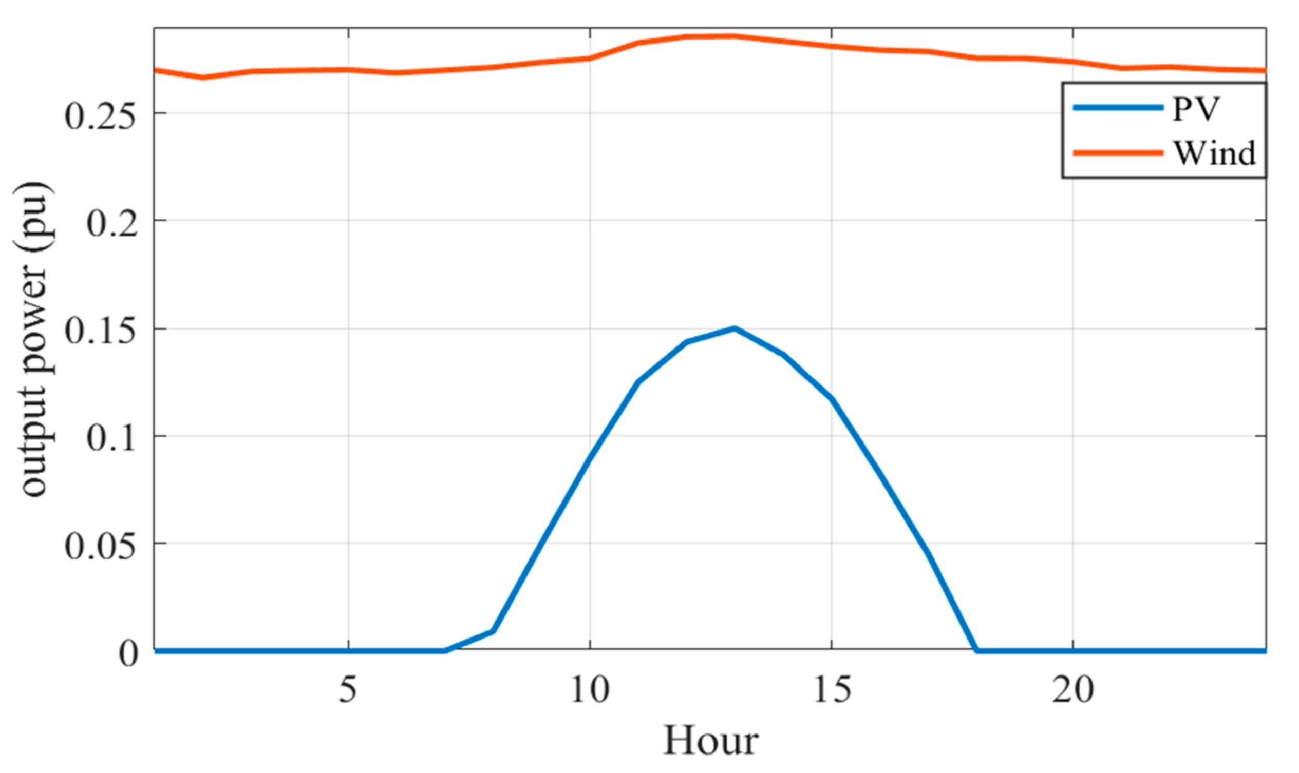Moreover, the output power of the wind turbine depends on the cut-in and cut-off speeds of wind in the location of the wind farm [37]. In the problem formulation of this article, the uncertainty of the PV and wind turbines’ electric power generation is not considered. Instead, constant models are used for the PV and wind energy sources according to the availability curves shown in Figure 1, which were provided in [25].

In the third part of the problem formulation after the optimal siting, the OPF problem was resolved after some modifications in load values, as a result of RESs’ addition to the standard IEEE test systems studied.

Various scenarios are considered to investigate the impact of the addition of RESs on reducing the cost of conventional generating fuel. These are four different scenarios—OPF problem with the variable load during the day without adding wind or PV sources to systems; OPF problem with variable load, with only the addition of a PV energy source that is associated with buses obtained in the second part of problem formulation (optimal sitting part); OPF problem with variable load with only the addition of a wind energy source; and finally, OPF problem with variable load with the addition of PVs and wind energy sources together to studied systems.

In all parts of the problem formulation, the design variables are bounded by their limits. The constraints that are given in (3), (4) and (6) are satisfied by the power flow in the MATPOWER toolbox [38,39,40] in MATLAB. A penalty function (pen) is added to the objective function to guarantee that the results of the other dependent variables are limited to their boundaries, and to confirm that there are no violations of limits. The violated solutions are rejected by the penalty term in the equation of the fuel cost, as specified in (9).

$$pen=k_v{\displaystyle \sum }_{i=1}^{n_{buses}}\left[\begin{array}{c}max\left(0,V_i-V_i^{max}\right)\\ +max\left(0,V_i^{min}-V_i\right)\end{array}\right]+k_l{\displaystyle \sum }_{j=1}^{n_{br}}\left[max\left(0,S_j-S_j^{rated}\right)\right]$$

(9)

where $k_v$ and $k_l$ are positive integers of very large values. $n_{buses}$ and $n_{br}$ are the number of buses and branches, respectively.

3. Hunger Games Search (HGS) Optimization Algorithm

The HGS is classified as a population-based optimization algorithm. It is simple to implement, stable, and competitive when used to solve the optimization problems with the constraints [23]. The principles of the HGS algorithm rely on the hunger-motivated behavior of the animals. It is inspired by the animals’ social characteristics, while the food exploration depends on their hunger level. This dynamic optimization algorithm follows the concept of “Hunger” as a vital inspiration for activities in the lives of beings. The HGS optimization algorithm simulates the hunger by designing weights to represent the hunger affect the search steps. The algorithm obeys the logical rules used by the animals. Its activities are considered adaptive evolutionary, as the animals try to secure more opportunities for food possession.

3.1. The Logic of Search, Behavioral Choice, and Hunger-Driven Games

Animals live according to the rules that depend on the environment in which they live. Rules control animal choices and the evolution of their style. Hunger stimulates animal choices and activities. Hunger also affects the anxiety of animals and worry from the hunters. Animals look for food sources when faced with a lack of calories. They should look for food besides moving around environments to switch between exploration and defense to change nutrition plans smoothly. Social life supports animals in the possibility of escaping from hunters and exploring food sources. This social lifestyle improves the chance of animals surviving. In nature, better-health animals can get food and, therefore, they live more likely than vulnerable animals. These hunger games are called in nature where the wrong choices can lead to death. Not only is animal behavior affected by hunger, but also by the fear of hunters. The more severe the hunger, the stronger the food search. Therefore, the animal is doing more effort to find food shortly before his death. The proposed optimization method depends on logical options and species movements.

3.2. Mathematical Model

This sub-section introduces the important mathematical equations of the HGS optimization algorithm. The mathematical model is built based on hunger-motivated actions.

Approaching the food: It is assumed that all the individuals help and cooperate socially. The pivotal equation of the proposed HGS optimization algorithm which represents the individual cooperative communication is given in (10) [23]; thus:

$$\overrightarrow{X\left(t+1\right)}=\left\{\begin{array}{l}{\mathrm{Game}}_1:\overrightarrow{X\left(t\right)}\left(1+\mathrm{randn}\left(1\right)\right),r_1<l\\ {\mathrm{Game}}_2:\overrightarrow{W_1}\overrightarrow{X_b}+R\to \overrightarrow{W_2}\left|\overrightarrow{X_b}-\overrightarrow{X\left(t\right)}\right|,r_1{>l,r}_2>E\\ {\mathrm{Game}}_3:\overrightarrow{W_1}\overrightarrow{X_b}-R\to \overrightarrow{W_2}\left|\overrightarrow{X_b}-\overrightarrow{X\left(t\right)}\right|,r_1{>l,r}_2<E\end{array}\right.$$

(10)

$r_1$ and $r_2$ are random numbers between [0, 1]. $t$ is the number of the current iterations. $\overrightarrow{W_1}$ and $\overrightarrow{W_2}$ are the weighting factors of hunger. $\overrightarrow{X_b}$ denotes the best individual location at the current iteration.

In (10), individuals are looking for locations close to the best solution, as well as searching for other locations far from the best solution. This ensures that the exploration process covers the entire search space to meet its limits.

The hunger role: The starvation features of the population in the exploration field are mathematically expressed and $\overrightarrow{W_1}$ is calculated by (11) [23].

$$\overrightarrow{W_1\left(i\right)}=\left\{\begin{array}{l}hungry\left(i\right)\frac{N}{SHungry}{\times r}_4{,r}_3<l\\ {1,r}_3>l\end{array}\right.$$

(11)

Meanwhile, $\overrightarrow{W_2}$ in (10) is calculated as shown in (12):

$$\overrightarrow{W_2\left(i\right)}=2\left({1-e}^{-\left|hungry\left(i\right)-SHungry\right|}\right)r_5$$

(12)

where $hungry$ is the $hungr$ of the population. $r_3$, $r_4$, and $r_5$ are random values between 0 and 1. $\mathit{N}$ is the population size. $SHungry$ defines the summation of the populations’ hungry feelings.

The $hungry\left(i\right)$ can be represented mathematically as follows (13) [23]:

$$hungry\left(i\right)=\left\{\begin{array}{l}0,\forall AllFitness\left(i\right)==BF\\ hungry\left(i\right)+H,\forall AllFitness\left(i\right)!=BF\end{array}\right.$$

(13)

where $AllFitness\left(i\right)$ is the fitness of the current iteration. At every iteration, the best population’s hunger is set to 0. Meanwhile, the new hunger ($H$) is added to other populations according to the original hunger. The H values that correspond to each population are not the same. The pseudo-code of the HGS optimization algorithm is presented in Algorithm 1.

Algorithm 1. Pseudo-code of HGS.

Initialize the parameters and positions

while (t ≤ T)

Calculate the fitness of all individuals

Update BF, WF, Xb, BI

Calculate the Hungry, W1, W2

for each individual

Calculate E

Update R and positions

end for

t = t + 1

end while

Return BF and Xb

3.3. Chaotic Hunger Games Search Optimization Algorithm (CHGS)

In the meta-heuristic optimization algorithms, the initial population is set randomly within specified upper and lower bounds. The performance of optimization algorithms is greatly influenced by the initial configuration of agents. The better the initial population, the better the results. In this research, the initial population is improved using chaotic maps. The principle of modifying the initial population by the chaotic maps in the metaheuristic algorithms was discussed in [39,40].

The discussion in [40] led to the fact that the logistic chaotic maps are the best among the recent chaotic maps because of the computational efficiency, due to the random initialization of numbers near 0 and 1. This type of chaotic mapping can be represented mathematically, as given in (14) [24].

$$\begin{gathered} y_1=\mathrm{rand}, \\ {y}_{i+1}{=4y}_i\left({1-y}_i\right),\forall i\in N \end{gathered}$$

(14)

where rand is a vector set randomly from 0 to 1. After that, the initial population of the proposed CHGS optimization algorithm is defined by replacing the initial population determined by the HGS with the values obtained by such a type of chaotic mapping. This replacement of the initial population improves the simulation performance of the HGS. The flowchart of the power flow problem using the CHGS optimization method is shown in Figure 2.

4. Simulation Results

The steps of using the CHGS to solve the OPF problem are as follows: the number of populations, the dimension of the problem, the constraints of the design variables, and the maximum number of iterations are defined and set. The CHGS generates the initial population using chaotic maps. The OPF is run by the MATPOWER toolbox [38]. The values of the active power generated, obtained by the results of the OPF, are used to calculate the objective function (cost function). Then, the other populations are used to solve the OPF iteratively by the MATPOWER, and the output from the OPF in each iteration is used to calculate the objective function. If the cost of the current iteration is less than the cost of the previous one, it replaces the old result. These steps end if the maximum number of iterations is reached, as shown in Figure 2.

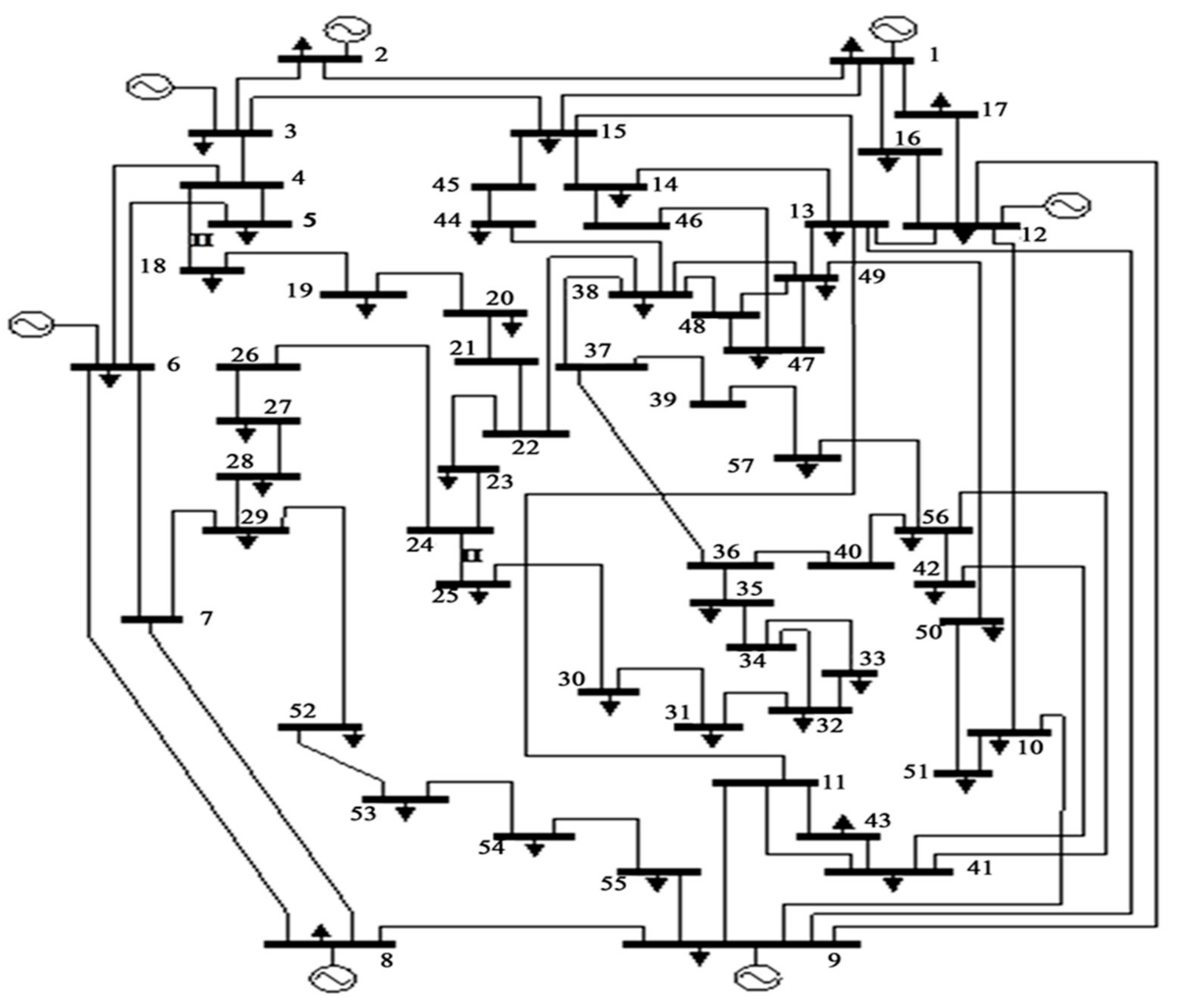
To verify the applicability of the developed CHGS optimization algorithm in the field of modern electrical power systems, it is used to solve the OPF, with the three scenarios of the optimization problem presented before in the problem formulation section. The standard test systems IEEE 57-and 118-bus are used in this study. This section of the paper shows simulation results for the three scenarios of the optimization problem in the following subsections. In

Table 1. Data of the two studied systems.

Data/System	57-Bus System [5]	118-Bus System [5]
Number of buses	57	118
Number of generators	7	54
Number of branches	80	186
Number of transformers	17	9
Number of loads	42	99
Connected loads (MVA)	1250 + j336.4	4242 + j1438
Power losses (MVA)	16 + j72.97	132.86 + j783.79

, the main data of the first and second studied systems are presented [5]. The data tabulated include the number of buses, branches, transformers, loads. As a sample of the studied systems, the single line diagram of the IEEE 57-bus system is presented in Figure A1 in Appendix A at the end of this article, just before the references section. The values of the loads and the constraints of the voltages at each bus for the two studied systems are also included in two separate tables, in

Table A1. Voltage constraints, and load data of each bus for the 57-bus system.

Bus No.	Voltage (p.u)		Load
	Min	Max	Active Power (MW)	Reactive Power (MVAR)
1	0.9	1.1	55	17
2	0.9	1.1	3	88
3	0.9	1.1	41	21
4	0.9	1.1	0	0
5	0.9	1.1	13	4
6	0.9	1.1	75	2
7	0.9	1.1	0	0
8	0.9	1.1	150	22
9	0.9	1.1	121	26
10	0.9	1.1	5	2
11	0.9	1.1	0	0
12	0.9	1.1	377	24
13	0.9	1.1	18	2.3
14	0.9	1.1	10.5	5.3
15	0.9	1.1	22	5
16	0.9	1.1	43	3
17	0.9	1.1	42	8
18	0.9	1.1	27.2	9.8
19	0.9	1.1	3.3	0.6
20	0.9	1.1	2.3	1
21	0.9	1.1	0	0
22	0.9	1.1	0	0
23	0.9	1.1	6.3	2.1
24	0.9	1.1	0	0
25	0.9	1.1	6.3	3.2
26	0.9	1.1	0	0
27	0.9	1.1	9.3	0.5
28	0.9	1.1	4.6	2.3
29	0.9	1.1	17	2.6
30	0.9	1.1	3.6	1.8
31	0.9	1.1	5.8	2.9
32	0.9	1.1	1.6	0.8
33	0.9	1.1	3.8	1.9
34	0.9	1.1	0	0
35	0.9	1.1	6	3
36	0.9	1.1	0	0
37	0.9	1.1	0	0
38	0.9	1.1	14	7
39	0.9	1.1	0	0
40	0.9	1.1	0	0
41	0.9	1.1	6.3	3
42	0.9	1.1	7.1	4.4
43	0.9	1.1	2	1
44	0.9	1.1	12	1.8
45	0.9	1.1	0	0
46	0.9	1.1	0	0
47	0.9	1.1	29.7	11.6
48	0.9	1.1	0	0
49	0.9	1.1	18	8.5
50	0.9	1.1	21	10.5
51	0.9	1.1	18	5.3
52	0.9	1.1	4.9	2.2
53	0.9	1.1	20	10
54	0.9	1.1	4.1	1.4
55	0.9	1.1	6.8	3.4
56	0.9	1.1	7.6	2.2
57	0.9	1.1	6.7	2

in Appendix A.

As mentioned in the problem formulation section, the output power of each conventional generator is the design variable of the optimization problem. The simulation results of the three parts of the OPF optimization problem are explained in detail in the following subsections.

4.1. Base Case

The values of the best cost and best design variables obtained by the CHGS and other optimization techniques for the 57-bus and the 118-bus systems are presented in

Table 2. Optimal cost and design variables for the 57-bus system.

Generator Power (MW) at Bus	CHGS	GA	PSO [5]	HHO [3]
1	144.856065349	151.43944	153.41	144.89
2	93.0378363798	85.655155	0.00	94.85
3	45.2090447019	47.316627	47.07	45.08
6	68.2622752728	63.81441	61.09	65.90
8	457.026753271	471.12909	550.00	457.17
9	95.8566504056	75.268325	89.58	96.01
12	365.956944195	375.58131	374.31	366.24
Min cost (USD/hr)	41,872.90323	41,891.3742	42,262.61	41,873.06

and

Table 3. Optimal cost and design variables for the 118-bus system.

Generator Power (MW) at Bus	CHGS	GA	PSO
1	45.1280617027845	42.80843285	69.35736953
4	0	40.46726603	53.66406009
6	0	55.63989136	62.17215812
8	0	43.75528479	48.57892294
10	415.078573959537	263.0082435	0
12	89.2093137534019	73.4612556	91.82476326
15	0	71.50087072	54.09869923
18	51.1442426543932	40.50725262	100
19	0	30.79849664	0
24	0	51.10298629	0
25	202.066133641544	156.8538738	214.1341696
26	291.435485752547	136.8723279	0
27	0	39.63301115	28.14707861
31	0	33.53374789	7.457592479
32	0	35.67988555	100
34	0	48.36991819	100
36	52.6419746871120	42.5987049	0
40	0	32.43323935	41.61653112
42	0	34.42893636	100
46	20.3002706909648	33.19389347	19.08021288
49	207.252076963502	143.2983532	192.6388498
54	53.8043135610641	64.86753545	0
55	0	40.89349546	22.03011641
56	0	56.95884321	100
59	158.681203488787	112.15389	149.5723921
61	156.137895654654	104.6146765	148.2439412
62	0	45.70804411	0
65	370.286376438208	243.956903	352.4901168
66	368.272586926582	238.3546723	349.5263973
69	474.793720966816	241.9215895	451.7022087
70	0	61.23232172	0
72	12.7542211358947	42.53966077	100
73	0	36.76016444	0
74	0	36.59176546	0
76	39.7126044650688	46.35949401	0
77	0	58.62085889	0
80	450.443391212072	232.9528141	431.3098239
85	0	30.97517145	0
87	0	19.6315873	0
89	512.008503437726	385.117137	491.7252876
90	0	60.1034387	0.486243854
91	0	54.58481294	0
92	0	41.33189298	0
99	0	64.40857576	0.150287884
100	241.441910559835	136.2823639	226.413526
103	40.1846126066996	58.18509146	37.66294986
104	0	41.52387218	100
105	0	41.38774942	0
107	0	52.22079896	13.81565399
110	0	35.33619871	0
111	36.3598190416225	48.42831027	36.33637828
112	57.9142560051964	46.51878285	0
113	0	35.75126213	23.31851727
116	0	44.71488715	0
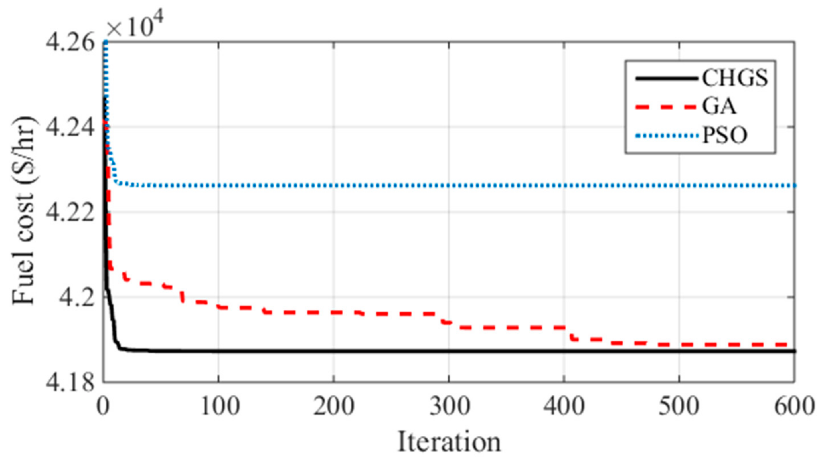
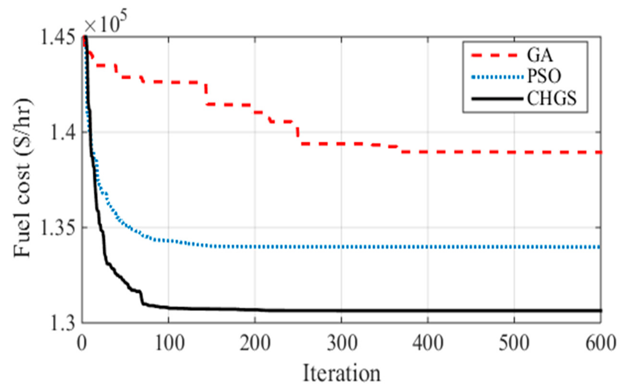
Min cost (USD/hr)	130,640.2534064	138,991.2993	133,976.07655089

, respectively. The performance of the CHGS in terms of the convergence in case of the 57-bus and the 118-bus systems are shown in Figure 3 and Figure 4, respectively, and it is compared with the convergence rates of the GA and the PSO.

In the case of the 57-bus system, the proposed CHGS optimization algorithm achieved a reduction in the cost function by 0.044% compared with the GA, and by 0.922% when compared with the PSO. The CHGS needed fewer iterations to settle. The GA algorithm needed about 400 iterations to reach its steady-state result. Moreover, the PSO converges fast, but its steady-state result is worse than the CHGS steady-state one. Meanwhile, in the case of the 118-bus system, the GA algorithm needs more iterations to settle, and it reaches the worst result of the three compared methods. The PSO convergence performance is similar to that of the CHGS algorithm, but the steady-state result obtained by the CHGS is better. The CHGS algorithm achieved a reduction in the cost by 3.9% compared with the GA, and by 2.48% when compared with the PSO. Besides, it is observed that the simulations of the two studied systems confirm the fast and smooth convergence of the proposed CHGS algorithm. Moreover, the CHGS can provide better results in the case of studying larger systems.

4.2. Optimal Siting of PV and Wind Energy Sources

In the second part of the optimization problem, the OPF problem is solved using the proposed CHGS, but for a different purpose. The goal in this part is to find the optimal bus to locate PV and/or wind energy sources. The optimal bus means the bus that achieves the minimum cost of power generation fuel in the system of the OPF problem. It is determined by checking the power generation fuel cost at each bus, and then, choosing the optimal one.

The optimal siting is targeted for the two systems under study, the 57-bus system, and the 118-bus system. First, the PV energy source is located, then the wind energy source. After that, both PV and wind energy sources are optimally located together. This is done by adding the PV source into the system, assuming that the wind source is already installed at the previously selected bus, as the wind energy source has a dominant effect on the reduction of the cost among the added RESs. The simulation results obtained for this part of the optimization problem for the two studied systems are presented in

Table 4. Optimal buses designated for RESs connection in the studied systems.

Test System	57-Bus System	118-Bus System
Optimal bus with PV power source	37	29
Optimal bus with wind power source	12	28
Optimal bus with mixed PV/wind sources	37/12	4/28

. These results are used in the third part of the optimization problem when the OPF is solved with variable load curves through the day, and with RES added to the studied systems. In this optimization problem, the PV and wind turbines are assumed to be added to the studied systems as a negative load changing in steps through the day, and the uncertainty of parameters was neglected for simplicity [41,42,43,44].

4.3. Different Scenarios of the OPF Problem Considering RESs

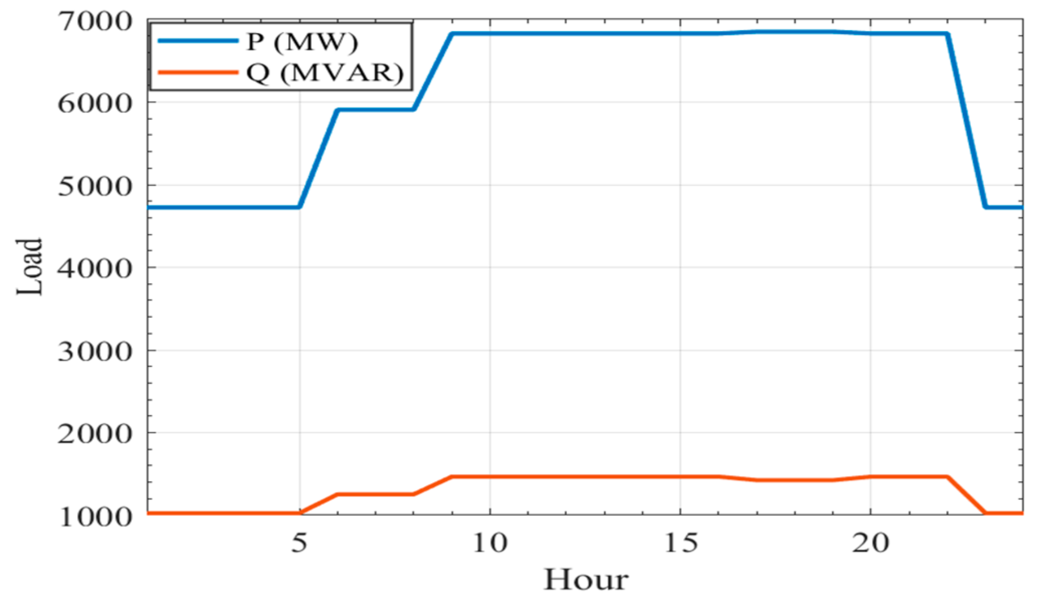
The third part of the optimization problem is solving the OPF problem with different scenarios. These different scenarios consider the system with hourly loads change. Values of the load of the 57-bus, and the 118-bus systems at each hour of the day are shown in Figure 5 and Figure 6, respectively [5].

Furthermore, the OPF problem is solved with the RESs, the PV, and wind energy sources, which are added to the systems individually or simultaneously. The aim in the third part of the problem is to investigate the impact of the addition of the RESs to the systems on the cost of conventional generator fuel. The RESs are supposed to be installed initially when included in the systems studied. 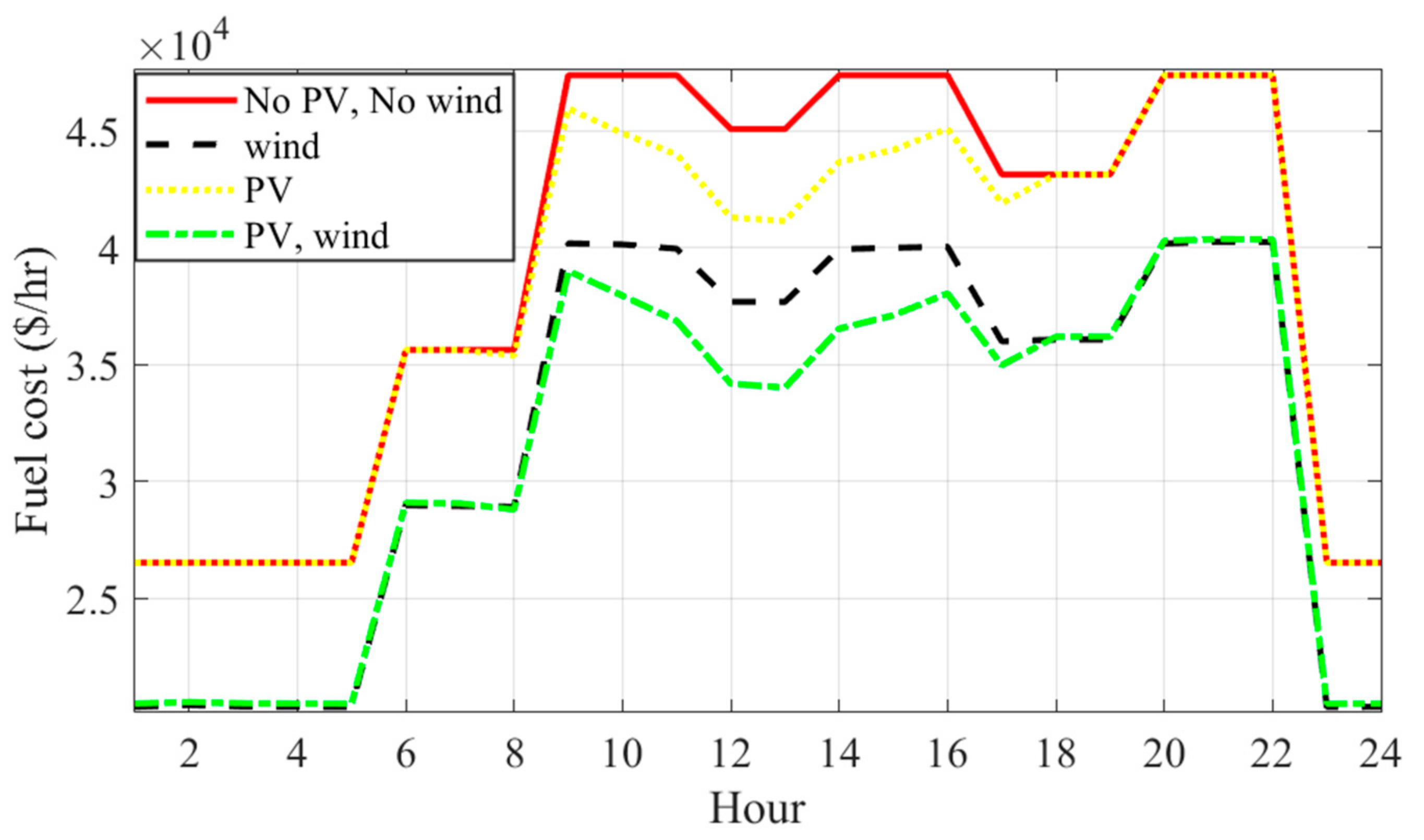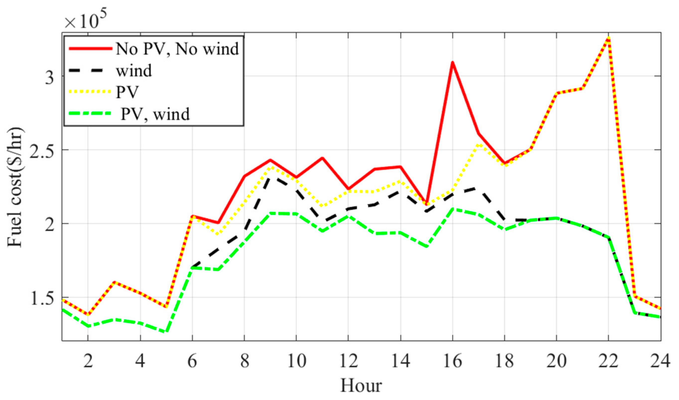This means that the initial capital costs of installing the RESs system have not been taken into account in this problem [44]. All scenarios are considered in the two studied systems; 57 buses, and 118 bus systems. These different OPF problem scenarios are resolved using the proposed CHGS optimization method.

The first scenario is the scenario where the OPF problem is solved with variable load and with no RES addition. In the second scenario, PV energy source is added to bus 37 in case of the 57-bus system, and to bus 29 in case of the 118-bus system. In the third one, a wind energy source is added to bus 12 in case of the 57-bus system, and to bus 28 in case of the 118-bus system. The last scenario investigates the OPF problem with the PV energy source installed on bus 37 and the wind energy source installed on bus 12, in the case of the 57-bus system. Meanwhile, in the 118-bus system, the PV energy source is installed on bus 4, and the wind energy source is installed on bus 28. Comparisons between these four scenarios in fuel cost through a typical day are demonstrated in Figure 7 for the 57-bus system. The hourly fuel cost comparison for all scenarios in case of the 118-bus system is also indicated in Figure 8. It is observed that the fuel cost is reduced between hours 9 and 18 after installing the PV energy source. Meanwhile, after the installation of the wind energy source, the fuel cost is reduced during the day. This happens due to the availability of wind energy all day, and the dependence of the output power from the PV energy source on solar irradiance.

4.4. Statistical Analysis

It is well known that metaheuristic optimization algorithms have a random nature. For this reason, the algorithms’ (CHGS, PSO, and GA) performances have been examined 20 times independently. The best, worst, mean, and median values are calculated and presented in

Table 5. Statistical measures of the results of the IEEE 57-bus system obtained with different algorithms over 20 independent runs.

Algorithm	Best	Worst	Mean	Median	Standard Deviation
CHGS	41,872.9032	41,872.90	41,872.90	41,872.90	4.76 × 10−10
PSO	4.20 × 104	42,404.38	42,133.54	42,172.18	162.0120
GA	41,891.3742	42,037.36	41,938.62	41,932.65	41.01491

for the IEEE 57-bus system, and

Table 6. Statistical measures of the results of the IEEE 118-bus system obtained with different algorithms over 20 independent runs.

Algorithm	Best	Worst	Mean	Median	Standard Deviation
CHGS	1.31 × ${10}^5$	1.37 × ${10}^5$	1.322 × ${10}^5$	1.3212 × ${10}^5$	7.97 × ${10}^2$
PSO	1.32 × ${10}^5$	1.36 × ${10}^5$	1.33 × ${10}^5$	1.33 × ${10}^5$	1.14 × ${10}^3$
GA	1.36 × ${10}^5$	1.40 × ${10}^5$	1.39 × ${10}^5$	1.39 × ${10}^5$	8.56 × ${10}^2$

for the IEEE 118-bus system. The standard deviation of the presented results has also been calculated.

It is clear from Table 5 that the standard deviation has the lowest value when the proposed CHGS algorithm is applied. It can be concluded that the deviation of the results obtained from each run is very small, so the results obtained are consistent. The same is achieved for the IEEE 118 bus system, as shown in Table 6. A non-parametric statistical test called Wilcoxon’s rank-sum test is also carried out. This test enables additional comparison between the proposed CHGS algorithm and PSO and GA algorithms. The corresponding p-values obtained by applying this test are presented in

Table 7. p-values obtained with Wilcoxon’s and Friedman’s rank-sum tests.

System	IEEE 57-Bus		IEEE 118-Bus
Algorithms/tests	CHGS vs. PSO	CHGS vs. GA	CHGS vs. PSO	CHGS vs. GA
p-value (Wilcoxon test)	6.40 × 10−8	6.50 × 10−8	2.73 × 10−1	1.43 × 10−7
p-value (Friedman test)	5.33 × 10−5		3.06 × 10−3

, with a 5% level of significance between the CHGS and other optimization methods. Besides, in addition to the previous non-parametric statistical analysis measures, a non-parametric statistical test called the Friedman test is also carried out to determine whether there is a difference between results in acceptance or not. Friedman tests classify values in each group (algorithm results in each run) from low to high. Each row is arranged separately. It then sums the ranks in each algorithm (column). The corresponding p-values obtained by applying this test are also presented in Table 7. The small p-values calculated validate the hypothesis that all differences between algorithm results due to random sampling can be rejected, and at least the proposed algorithm differs from the other based on convergence and other test results. To conclude, the results shown in Table 5, Table 6 and Table 7 validate the superiority of the CHGS algorithm over other considered algorithms in solving the investigated OPF problem under the conditions given in the problem formulation.

5. Conclusions

This paper has introduced an improved CHGS optimization algorithm to solve the optimal power flow problem. The systems used in this paper are the benchmark IEEE 57-bus and 118-bus test systems. The problem formulation was divided into three parts. The first part is the OPF with a base case, to investigate the convergence of the CHGS algorithm. In the second part of the problem formulation, an optimal allocation of the RESs was introduced by the CHGS algorithm. In the third part, different OPF scenarios were considered and solved by the CHGS. Different hourly load values and different levels of penetration of RESs into the studied systems were also considered. The penetration of the RESs resulted in considerable hourly cost reduction. The simulation results showed the applicability of the proposed CHGS optimization algorithm when used to solve the OPF problem in electrical power engineering fields. Compared with other optimization algorithms, the CHGS resulted in better convergence rates. In addition, it is simple to implement. The CHGS employment in the OPF problem has reduced the fuel cost by 0.04% up to 0.92% for the 57-bus system, and 2.4% up to 3.9% in the first part of the studied optimization problem. Finally, it can be recommended to try to apply the CHGS optimization algorithm to solve other problems in the scope of electrical engineering, energy, and other engineering fields in future research, while taking into account the uncertainty of the parameters and loads.