Beyond the Horizon, Backhaul Connectivity for Offshore IoT Devices

Abstract

The prevalent use of the Internet of Things (IoT) devices over the Sea, such as, on oil and gas platforms, cargo, and cruise ships, requires high-speed connectivity of these devices. Although satellite based backhaul links provide vast coverage, but they are inherently constrained by low data rates and expensive bandwidth. If a signal propagated over the sea is trapped between the sea surface and the Evaporation Duct (ED) layer, it can propagate beyond the horizon, achieving long-range backhaul connectivity with minimal attenuation. This paper presents experimental measurements and simulations conducted in the Industrial, Scientific, and Medical (ISM) Band Wi-Fi frequencies, such as 5.8 GHz to provide hassle-free offshore wireless backhaul connectivity for IoT devices over the South China Sea in the Malaysian region. Real-time experimental measurements are recorded for 10 km to 80 km path lengths to determine average path loss values. The fade margin calculation for ED must accommodate additional slow fading on top of average path loss with respect to time and climate-induced ED height variations to ensure reliable communication links for IoT devices. Experimental results confirm that 99% link availability of is achievable with minimum 50 Mbps data rate and up to 60 km distance over the Sea to connect offshore IoT devices.

1. Introduction

Ships and seacrafts near ports require high-speed wireless Communication to accommodate data-intensive services. On cargo vessels, cruise ships, and oil and gas rigs, Internet of Things (IoT) based lossless networks are necessary for smart operations [1]. Wi-Fi wireless communication systems using 2.4 GHz and 5 GHz bands are already installed on seaports for limited-range connectivity with nearby ships and vessels. The range of connectivity between the ships and seaports has gained persistent research interest due to the limited height of antenna towers installed on ships and curvature of earth [2,3,4,5]. Wireless connectivity around seaport is also limited due to line-of-sight (LOS) propagation between the transmitter and the receiver. Therefore, the range of wireless connectivity around seaport is typically limited within 10 km–15 km [6]. Various wireless channel models for over the Sea communication with limited range and availability are discussed in [7]. However, long-range communication coverage with high-speed backhaul connectivity is necessary for smart platforms used in remote monitoring and surveillance. Backhaul is a reliable, high data-rate link to provide remote connectivity over the Sea surface. Trade vessels approaching seaports need to be connected well in advance to reduce ship lane queuing time. With digitization of oil and gas platforms over the Sea, IoT devices are installed to provide smart production operations. IoT improves energy efficiency, remote monitoring, security, and control of physical assets on offshore platforms [8,9]. However, the conventional over the sea communication techniques are not appropriate for such sophisticated actions on remote offshore platforms.

In tropical regions of the World, occurrence of Evaporation Duct (ED) layer over the sea is a common phenomenon. Wireless signal trapped in the ED can propagate beyond the horizon and cover vast distances with very less attenuation. In [10,11,12], Australian Institute of Marine Science (AIMS) has performed experiments at 10 GHz frequency band to establish long-range communication links utilizing ED. In addition, many articles are published on ED based measurements and predictions to establish a long-range radio link using ED [13,14,15]. Limited measurements in ED are also performed and path loss variations are predicted through machine learning algorithms [16,17]. The climatology of ED and its percentage of occurrence is important for the signal propagation in ED. 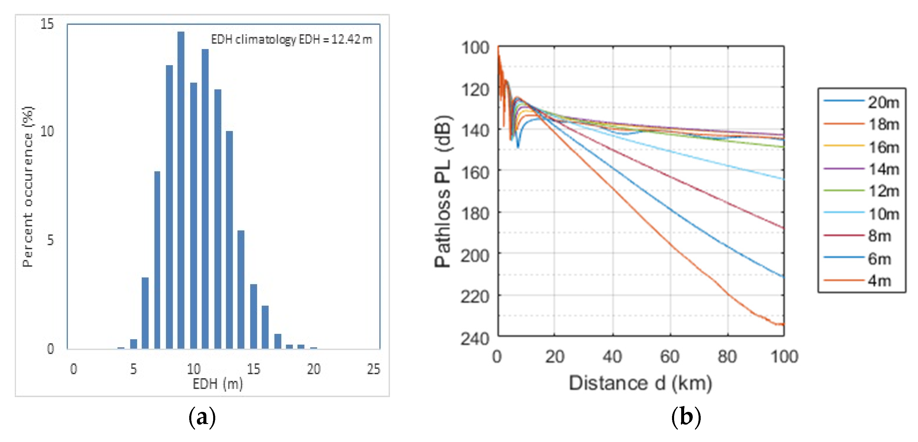Therefore in [18], a new ED climatology measured within the Malaysian Sea region of South China Sea is presented. However, the average height of the evaporation duct was 12.42 m and its occurrence vary from 4 m to 20 m [18]. The authors conducted an experimental study in Malaysian region of South China Sea using ED climatology. 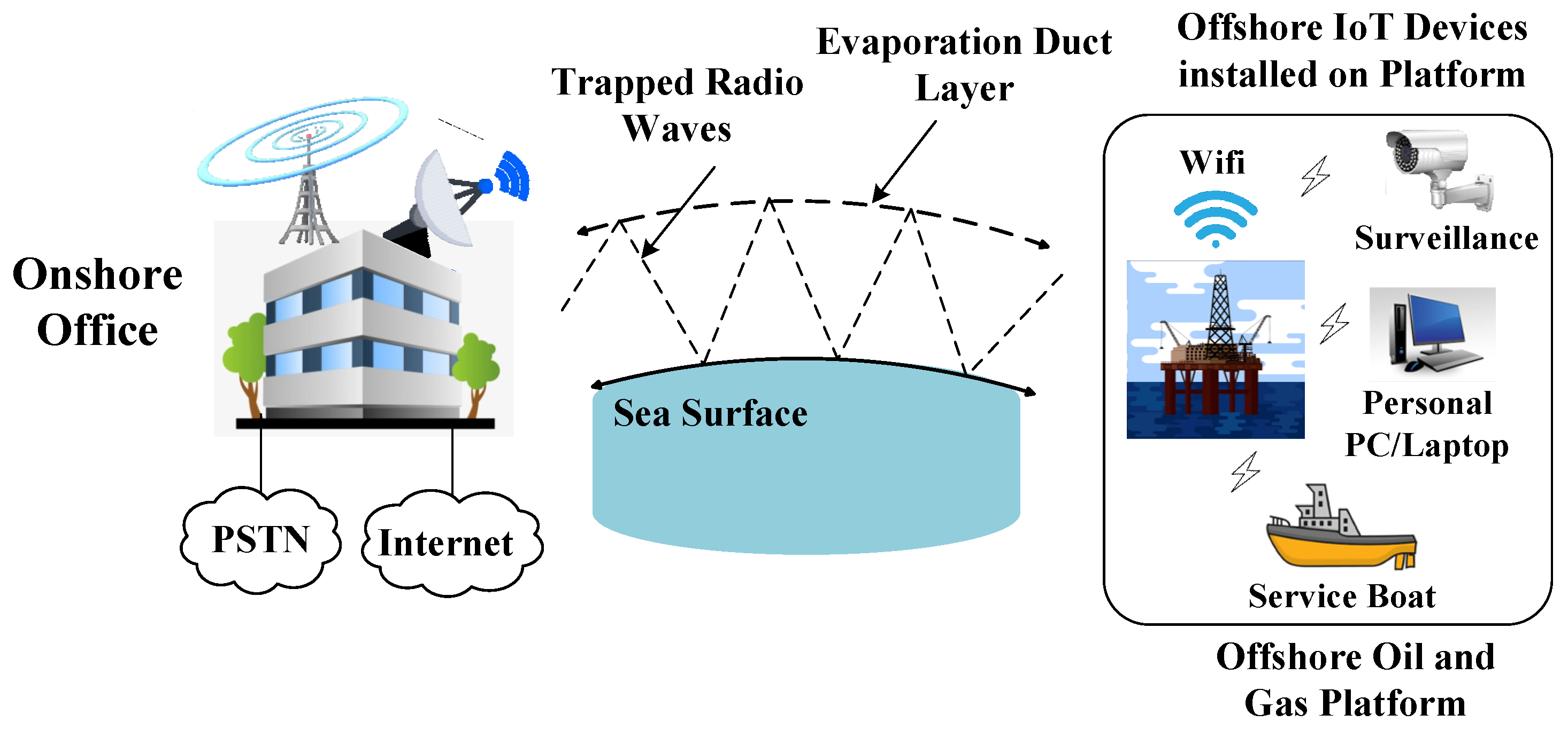The authors reported that the ED availability and capacity based on fade margin can be estimated correctly using path loss measurements [15]. Therefore, it is necessary to extend high-speed connectivity range between the seaports and the moving vessels with low altitude antennas. A reliable backhaul link via ED can provide high data rate connectivity to IoT based network on an offshore platform, cargo vessel, or cruise ships, as shown in Figure 1.

Another advantage of propagating in ED is that we require low antenna height compared to conventional line of sight based backhaul links. Due to this fact, we require a low-cost infrastructure and low power to achieve beyond the horizon offshore IoT devices connectivity. The energy is trapped between the sea surface and the ED layer with very less attenuation and enhanced signal strength. By keeping in view above stated requirements of targeted studies on over the sea IoT devices connectivity using ED, we gather real-time experimental measurements for large-scale characterization in the Malaysian Sea region and perform extensive simulations to explore backhaul connectivity of IoT devices using ED. Therefore, the aim of this paper is to analyze the average measured path loss in ED at varying distances and then predict additional path loss variations, also termed as slow fading based on the probability of occurrence of ED height changes. Based on complete path loss information, availability, and capacity of a beyond the horizon backhaul link is calculated to establish connectivity to offshore IoT devices. Main contributions of the paper are:

• The efficiency of the backhaul connectivity link for offshore IoT devices is measured using average values of path loss in ED at varying distances.
• Due to ED height variations, the additional path loss or slow fading with respect to time is estimated using ED climatology [15]. For varying ED climatology, we extended our work in [15] to compute fade margin at 5.8 GHz frequency.
• Using measured average path loss and additional slow fading, we have estimated a data rate of 50 Mbps for a 60 km beyond the horizon link to offshore IoT devices with 99% availability.

Rest of the paper is organized as follows: Section 2 presents average path loss prediction in ED at 5.8 GHz using PE tool-based simulations, verified with field measurements, and then fitted with Simplified Path Loss model. In Section 3, additional slow fading in ED is predicted at 5.8 GHz using simulations and we thoroughly analyzed the data. Section 4 has the link budget calculations to estimate availability vs. capacity in ED for 30 km, 40 km, 55 km, 64 km, and 80 km ranges. We conclude the paper in Section 4 along with future research directions.

2. Methodology

For any IoT network on an oil and gas platform, cruise ship or cargo vessel on the Sea, the high-speed, long-range backhaul wireless communication link can be established using ED. The only parameter that varies for a high data rate, reliable link is path loss. Average path loss is predicted using parabolic equation and measured over the Sea. There is additional slow fading induced because of climatic variations which is calculated based on the ED height variations over the Sea.

2.1. Average Pathloss Using PE Simulation Tool

Average path loss in ED at 5.8 GHz can be predicted using refractivity-based simulation models available in literature. Advanced Refractive Effects Prediction System (AREPS) software [19] based on Parabolic Equation (PE) model is used to predict average path loss for varying distances. We have simulated and calculated path loss variations for a 100 km distance over the Sea in the Malaysian region of the South China Sea with receiver antenna height of 4 m. The frequency is set at 5.8 GHz and the average value of day and night ED height variation in the Malaysian region is used to plot P.E based pathloss. The signal is trapped between the sea surface and ED layer to propagate beyond the horizon up to 100 km.

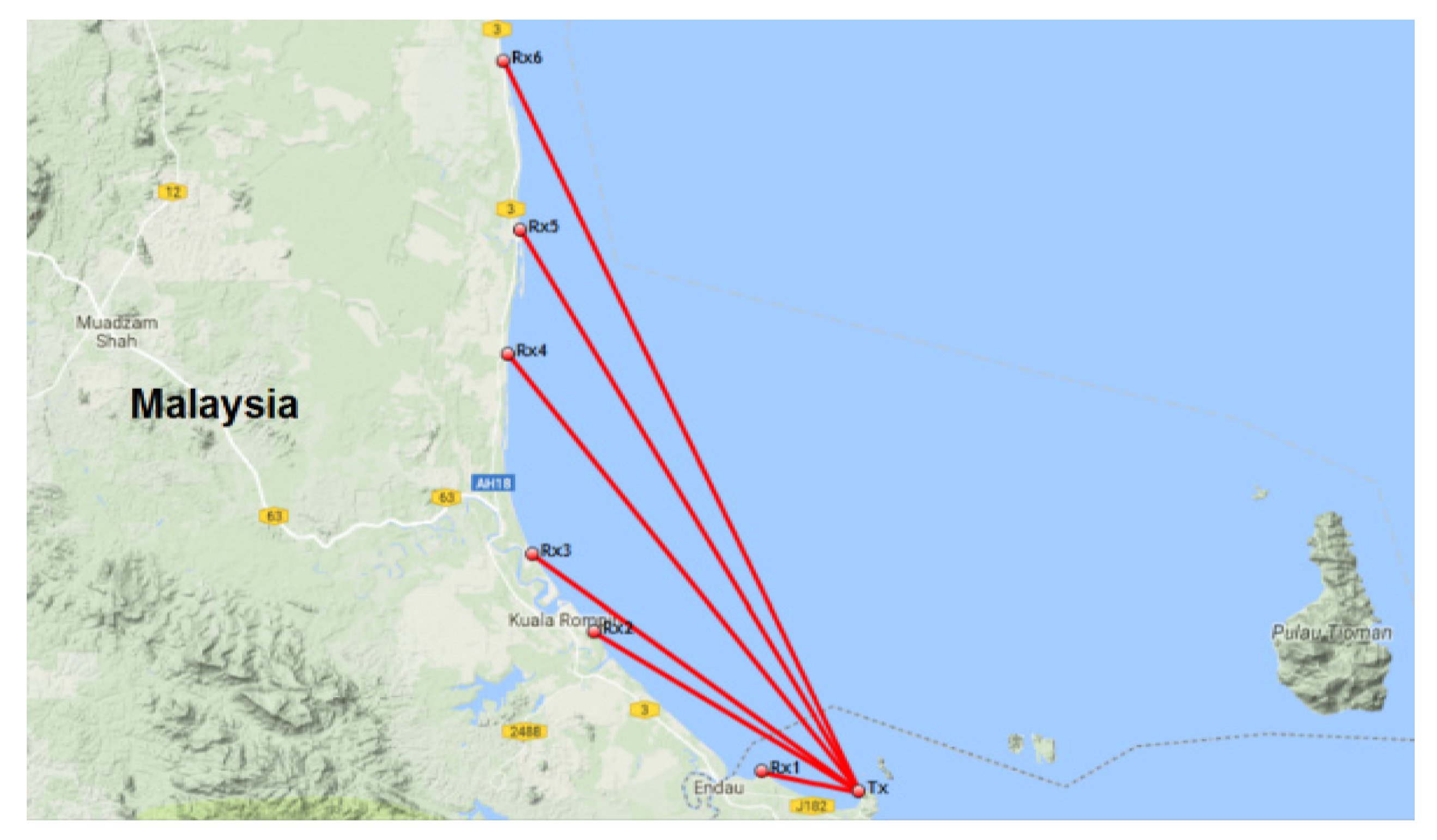
2.2. Average Measured Pathloss Campaign

Average measurement of path loss campaign is carried out in the Malaysian region over the South China Sea as shown on a Google map in Figure 2.

The received signal level is measured using a spectrum analyzer. System constants, listed in

Table 1. Constant parameter values for measurement campaign.

Parameter	Definition	Constant Value
PT	Transmitted Power (dBm)	23
GT	Tx Horn Antenna Gain (dBi)	12
GR	Rx Horn Antenna Gain (dBi)	12
GPA	Power Amplifier Gain (dB)	33
GLNA	Low Noise Amplifier Gain (dB)	26
IL	Insertion Loss (dB)	22

, are used to calculate propagation pathloss. System constants such as power transmitted $P_T$, antenna gains $G_T$ and $G_R$, power amplifier gain $G_{PA}$, low noise amplifier gain $G_{LNA}$ are obtained from the manufacturer datasheet. Insertion Losses $IL$ includes Coaxial cable losses which are computed for both transmitter and receiver at 5.8 GHz. Pathloss in dB is computed using following equation:

$$PL\left(dB\right)=P_T+G_T+G_R+G_{PA}+G_{LNA}-IL-P_R$$

(1)

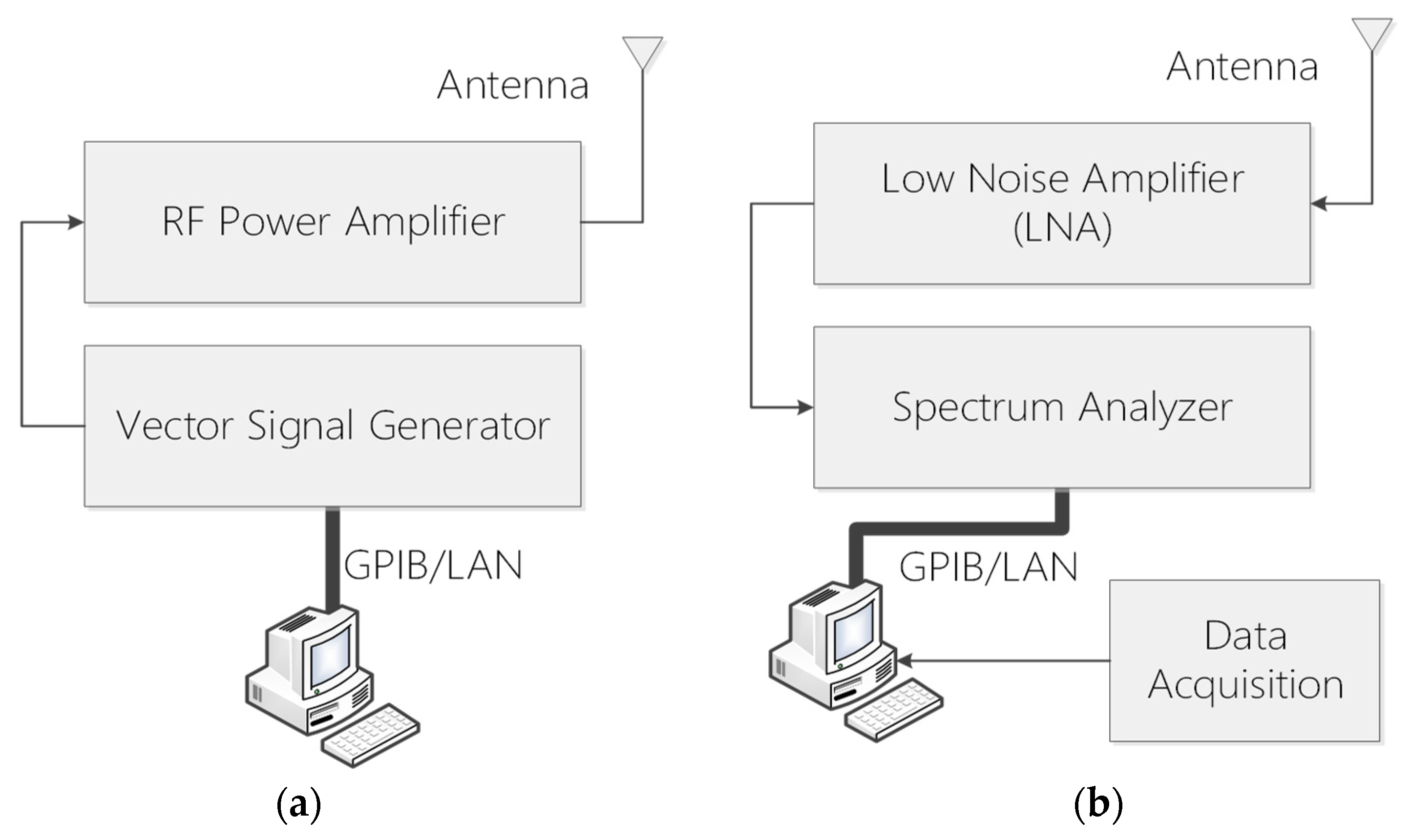
At the transmitter site in Figure 3a, Vector Signal Generator (VSG) is used to generate signal carrier frequency at 5.8 GHz with maximum transmit power of +23 dBm. Wideband power amplifier is used in series with VSG, having output power of 3 Watts, to make the total output power transmitted to be +33 dBm at 5.8 GHz. Broadband Horn Antenna with 12 dBi Gain is used to transmit the signal in the air. At the receiver site in Figure 3b, Spectrum Analyzer is used to receive the carrier signal with center frequency of 5.8 GHz. A Low Noise Amplifier (LNA) is used in series with Spectrum Analyzer, which provides an additional gain of 26 dB. Broadband Horn Antenna with 12 dBi Gain, similar to the transmitter, is used to receive the signal in the air. A MATLAB script featuring SCPI commands is used to control the instrument and to acquire discrete time data from Spectrum Analyzer. The center frequency and span of Spectrum analyzer is set to 5.8 GHz and 10 KHz respectively.

Once Received Signal Strength (RSL) is acquired from the spectrum analyzer, post-processing is performed to de-embed the system constants and to obtain propagation Pathloss. System constants include total power transmitted (P_T), antenna gains (G_T and G_R), low noise amplifier gain (G_LNA) are obtained from the manufacturer datasheet. L_T and L_R are the Coaxial cable losses at the transmitter and receiver respectively and are experimentally computed at 5.8 GHz. Pathloss was calculated by de-embedding constant values shown in Table 1.

The average path loss values were recorded for a short period of time during measurement and therefore, may vary with climatic conditions. Additional fading needs to be calculated over and above average measured path loss to accurately ascertain the fade margin required for a reliable backhaul link.

2.3. Additional Random Slow Fading ${\psi }_{dB}$

The slow fading in ED is climate-induced and relates to the percent of ED height occurrence. It is the combination of slow path loss fading and fast-instantaneous fading. The slow path loss fading distributions can be determined by understanding the changes in the average path loss value. With the change in ED height, the average path loss value also changes. The ED height variations are measured in a new climatology of South China Sea showing ED height profile in [15] as shown in Figure 4a. It is also evident that the changes in average path loss values due to slow fading are not related to distance. Instead, these are temporal variations. The transmitter and receiver are fixed and the change in average pathloss is only due to changes in ED characteristics, mainly its height. The fast-instantaneous fading on top of the slow fading is because of multipath effect within the channel created by sea wave movement.

To determine complete fading characteristics in ED, one needs to know the average path loss values with respect to distance along with the additional weather-dependent slow and fast fading due to multipath. The average path loss measurements help to determine the path loss exponent and type of fading. PE-tool based simulations using known ED climatology of the South China Sea, as shown in Figure 4b, can determine mean path loss and complete path loss variations. These slow path loss variations can be calculated using the best-fit distribution. The data acquired from simulations can be approximated with three-parameter (3-P) lognormal distribution. The probability density function for 3-P lognormal distribution is given in Equation (2),

$$f\left(x\right)=\frac{{\left(x-\gamma \right)}^{-1}}{\sigma \sqrt{2\pi }}exp\left(-\frac{1}{2{\sigma }^2}{\left[\ln \left(x-\gamma \right)-\mu \right]}^2\right)$$

(2)

where $x$ is in dB and $\sigma =$ continuous shape parameter ($\sigma >0$), representing swaying of the peak on the left. $\mu =$ scale parameter, represents width of peak that stretch or shrink the distribution. $\gamma =$ location parameter, is the starting location of the data ($\gamma \equiv 0$ yields the 2-P).

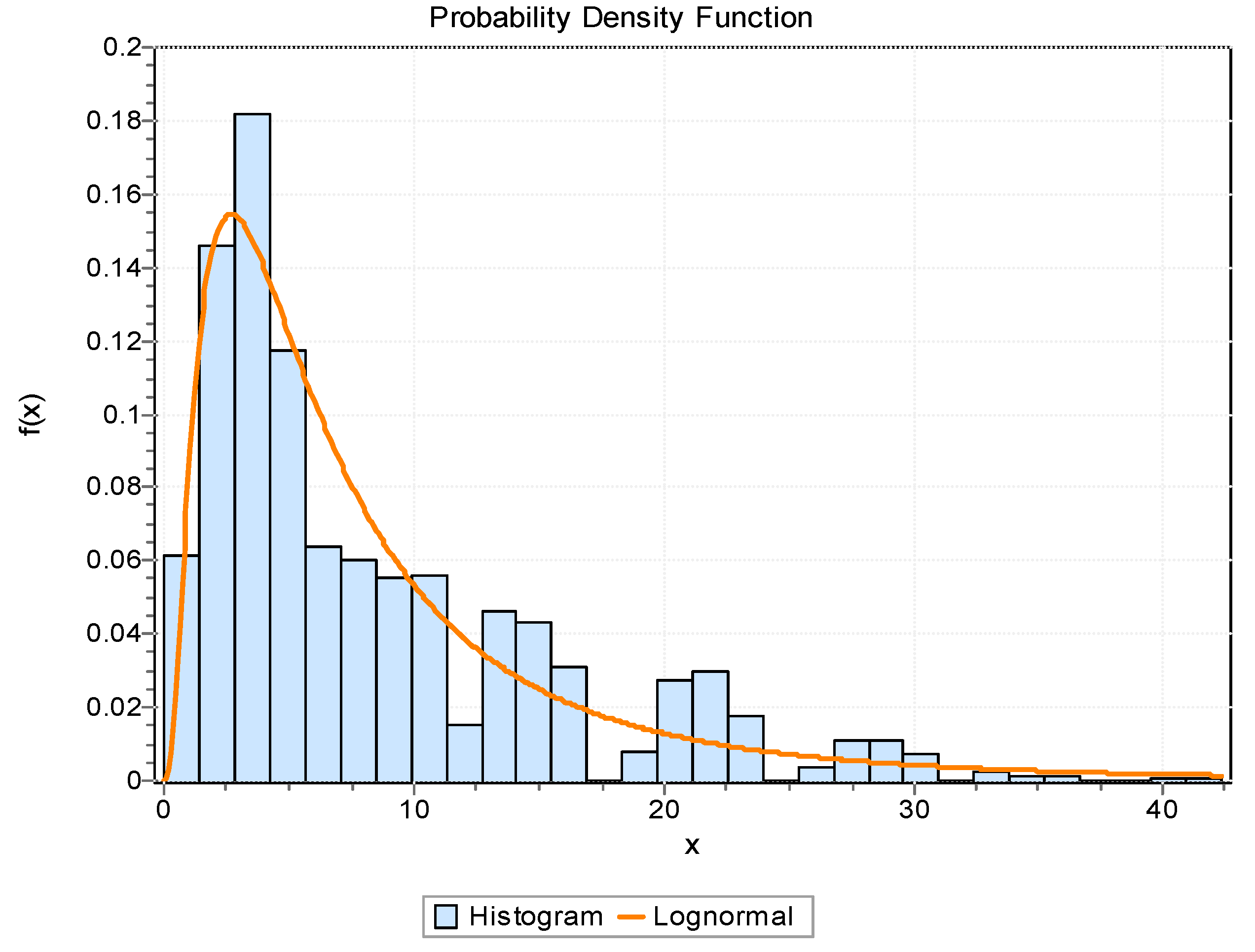
The shape of the pathloss distribution depends primarily on two parameters: $\mu$ and $\sigma$. We have calculated values of both parameters at each distance. The probability distribution of 3-P lognormal distribution is same as the 2-P lognormal distribution except the third location parameter, which depends on the distance between the transmitter and the receiver. For demonstration, a 2-P lognormal distribution at 40 km distance is shown in Figure 5. The average path loss varies up to 42 dB due to climate-induced changes in the ED. To calculate fade margin in addition to the average path loss value, the third parameter $\gamma$ can be neglected as in,

$$x^{\prime }=x-\gamma$$

(3)

Therefore, the equation can be represented as 2-P lognormal distribution,

$$f\left(x\right)=\left\{\frac{1}{x^{\prime }\sigma \sqrt{2\pi }}exp\left(-\frac{1}{2}{\left[\frac{ln\left(x^{\prime }\right)-\mu }{\sigma }\right]}^2\right)\right\}$$

(4)

The equation depends on the lognormal values of $\mu$ and $\sigma$. To calculate the parameter values in dB, we can use the following equations which is defined in [20] as,

$$mean={\mu }_{dB}=e^{\left(\mu +\frac{{\sigma }^2}{2}\right)}$$

(5)

$$variance={\sigma }_{dB}^2=e^{\left(2\mu +{\sigma }^2\right)}\left[e^{{\sigma }^2}-1\right]$$

(6)

From variance, one can calculate standard deviation as,

$${\sigma }_{dB}=\sqrt{e^{\left(2\mu +{\sigma }^2\right)}\left[e^{{\sigma }^2}-1\right] }$$

(7)

The cumulative distribution function (CDF) of lognormal can be used to determine the probability as,

$$F\left({\psi }_{dB}\right)=\frac{1}{\sigma \sqrt{2\pi }}\underset{0}{\overset{{\psi }_{dB}}{{\displaystyle \int }}}\frac{e^{\frac{-{\left(ln\left(x\right)-\mu \right)}^2}{2{\sigma }^2}}}{x}dx$$

(8)

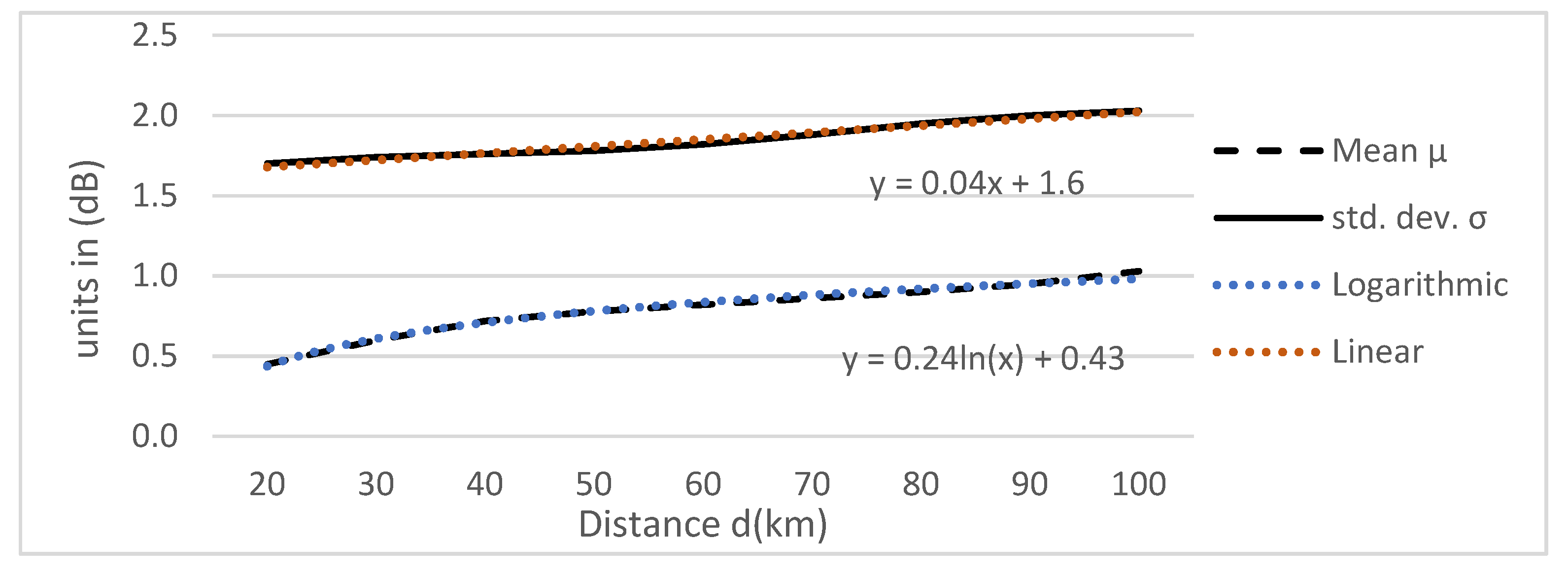
The shape of the path loss distribution depends primarily on two parameters scale $\mu$ and shape $\sigma$. We have calculated values of both parameters at each distance. A trendline for scale and shape values is obtained, which can be used to calculate lognormal distributions as shown in Figure 5. The path loss statistics provide equivalent probability distributions, which can be used to determine variance as in Equation (9). Standard deviation value at each distance is calculated based on its variance. Standard deviation value increases with increasing distance linearly, whereas mean of path loss increase lognormally with distance.

$${\sigma }_{dB}=0.04x+16$$

(9)

$${\mu }_{dB}=0.24ln\left(x\right)+0.43$$

(10)

where ${\mu }_{dB}$ is the mean of path loss, $x$ is distance and the value of standard deviation ${\sigma }_{dB}$ defines the variance of additional slow fading or path loss. This additional path loss needs to be added to the average measured path loss at varying distances. The availability of the system depends on the fade margin calculated considering these additional path loss variations. The outage probability of slow fading for a given threshold value of ${\psi }_{dB}=X_0$, and is defined as,

$$P_{avail}=1-P_{out}=p\left({\psi }_{dB}<X_0\right)$$

(11)

where, the distribution of ${\psi }_{dB}$ depends on standard deviation parameters ${\sigma }_{dB}$ and ${\mu }_{dB}$.

2.4. Link Budget for Avalibility and Capacity

For proposed link budget analysis to estimate availability and capacity in ED, we have considered constant parameters of a standard off-the-shelf Digital Microwave Radio (DMR) as described in

Table 2. Constant parameters and values of Wi-Fi equipment installed.

Constant Parameters	Value
Frequency	5.8 GHz
Transmit Power	30 dBm
Transmitter antenna Gain	20 dBi
Receiver Antenna Gain	20 dBi
Insertion Loss	2 dB
Bandwidth	20 MHz

. At 5.8 GHz frequency, W-Fi equipment installed on the seaport has maximum 1 Watt transmit power available. Horn antennas with wide beam width can provide gains up to 20 dBi. Insertion losses including cable and connector losses can be minimized to 2 dB. For a standard 20 MHz bandwidth with minimum receiver sensitivity of −94 dBm, a link budget in ED can be predicted. Link budget is based on a fade margin including both average path loss and additional fade margin due to climate-induced EDH variations.

Table 3. Fade margin for MIMO based Rayleigh fading model.

Availability (%)	Fade Margin (dB)
90	3
95	5
99	7
99.9	10
99.99	12

shows the additional fast fading margin required on top of slow fading in the proposed link budget. The fast-fading margin for a standard Wi-Fi is based on Multiple Inputs Multiple Outputs (MIMO) equipment which has at least 2 × 2 diversity as in [21].

3. Results

Results for predicted path loss using P.E based simulation tool, measured average path loss with additional slow fading and expected availability and capacity are shown in this section.

3.1. Predicted Pathloss Using P.E Simulation Tool

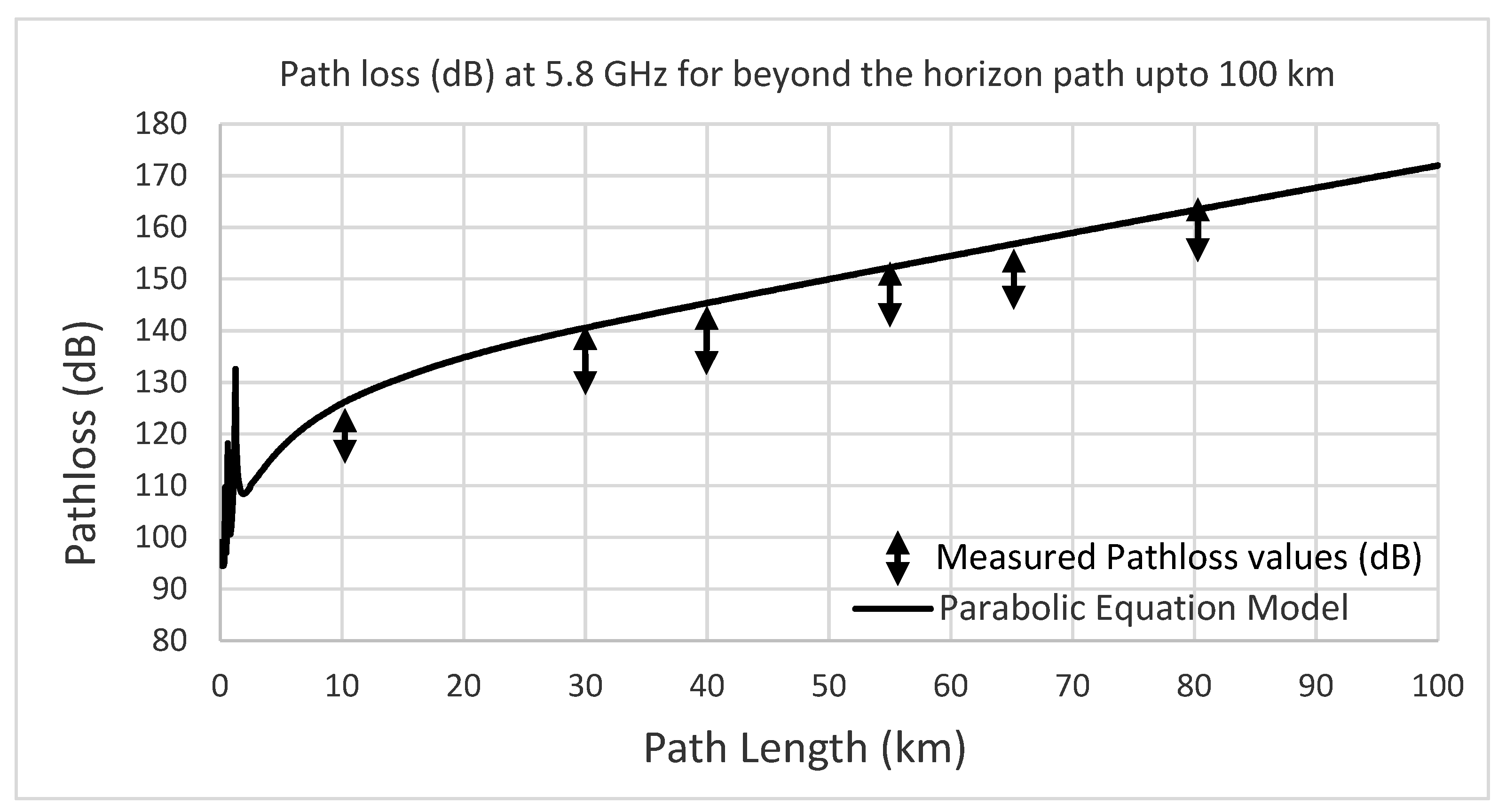
Simulation of average path loss prediction in ED at 5.8 GHz, shows a constant increase with respect to the distance as shown in Figure 6. The path loss increases up to 170 dB for a 100 km distance. Average path loss in ED at 10 GHz is much better than 5.8 GHz as in [22], but to utilize already installed Wi-Fi equipment around the seaport, 5.8 GHz frequency is chosen. This frequency has a much better response as compared to 2.4 GHz. As 5.8 GHz based equipment is already installed around the seaport, an extension in communication range is possible using propagation in ED with very low antenna heights.

3.2. Measured Average Pathloss at Various Distances

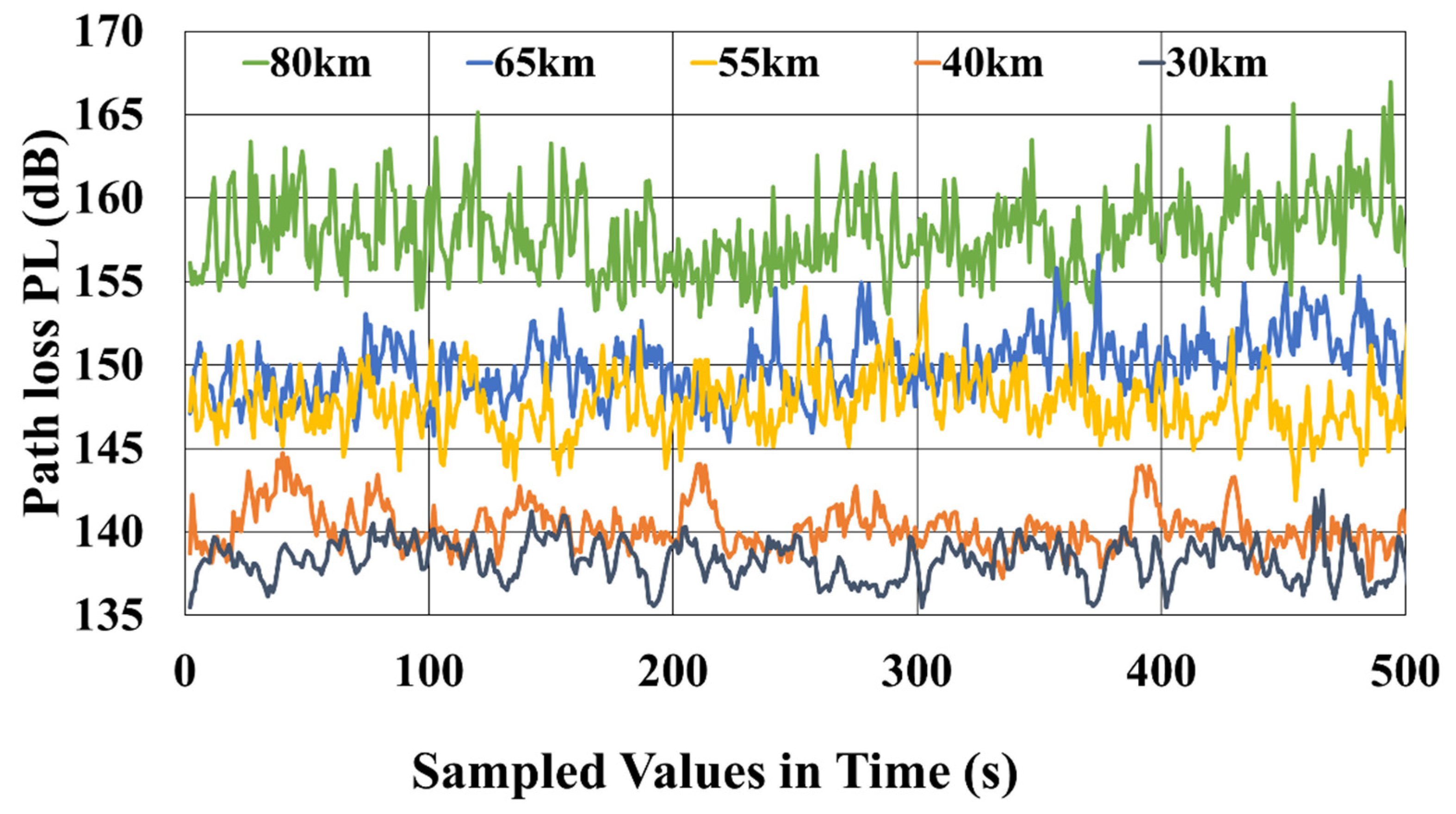
Experimental campaign to measure received signal level at regular intervals were conducted and several short-term measurements at six receiver sites were taken. Figure 7, shows the pathloss variations for all five beyond-the-horizon receiver sites, calculated from the measured received signal level. More than 500 sampled values were recorded at a carrier frequency of 5.8 GHz using spectrum analyzer. In all measurements, it was observed that the average path loss increased with the increase in distance. As 10 km distance was at LOS range, its average path loss variations are not shown. The average path loss for 30 km and 40 km were similar, although the path loss was slightly higher at 40 km distance. Average path loss values above 50 km, measured at 55 km and 65 km were at least 10 dB higher than 30 km and 40 km. The average measured path loss at 80 km distance was considerably very high with average value measured at 158 dBm. The measurements are taken for a time period. To know the complete variation of path loss in ED, one either needs long-term measurements with enough signal-to-noise (SNR) or fade margin.

3.3. Additional Slow Fading in the Channel

In addition to average path loss in ED, there is climate induced slow fading. It is noted that the changes in average path loss values due to slow fading are due to temporal changes rather than spatial. The transmitter and receiver are fixed and the change in average path loss is due to changes in ED characteristics only, mainly its height. The fast-instantaneous fading on top of the slow fading is also due to multipath effect within the channel due to sea wave movement. Additional slow fading at 40 km distance, approximated with 2-P probability distribution is shown in Figure 8. In Figure 8, it is visible that the PDF of the data is validated by Lognormal distribution (tail distribution). The 90% confidence interval lies up to 20 dB pathloss. However, we extended the confidence interval up to 40 dB to ensure 99% availability.

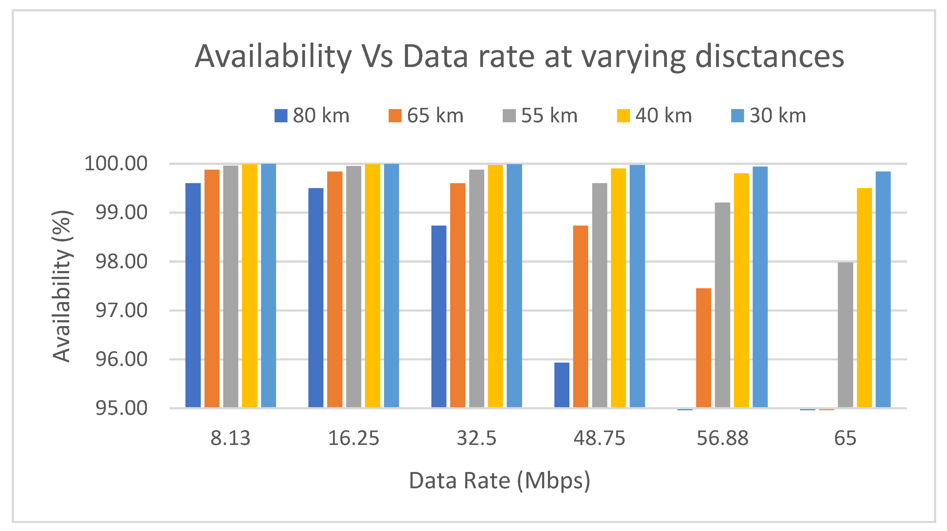
3.4. Availability and Capacity of the Backhaul Link

Availability of the backhaul link established in ED depends on the EDH variations. We have calculated availability considering the average measured path loss and predicted additional path loss variations based on the occurrence of EDH. Figure 9 shows the predicted availability vs. capacity for a 20 MHz channel bandwidth. Availability predictions for 30 km, 40 km, 55 km, 65 km, and 80 km distances use the average measured path loss with additional slow fading margin. For a 30 km link in ED using only 4 m high antenna towers, a minimum 99.7% availability is possible. For 40 km beyond the horizon distance, 65 Mbps utilizing 20 MHz bandwidth is possible with more than 99.51% availability. For a 50 Mbps data rate link an availability higher than 95% is possible at 80 km distance and with path length of 60 km, more than 99% availability is predicted in ED at 5.8 GHz. Therefore, the link at 60 km is likely to be in outage for only 1% of the time throughout the year.

With maximum transmit power of 1-Watt equivalent to +30 dBm and horn antennas providing 20 dBi gains one can establish a back haul link utilizing ED, which provides high availability of more than 99.5% up to 40 km at 65 Mbps and availability of 99% up to 60 km at 50 Mbps. For longer distances, up to 100 km, 99% availability is possible with least data rate of 8 Mbps. For a low data rate, less fade margin is required, so a higher availability is possible. Whereas, for a higher data rate, higher Quadrature Amplitude Modulation (QAM) requires large fade margin, reducing availability of the backhaul link. For a higher data rate, either higher transmit power or increase in antenna gain is required to achieve similar availability. Therefore, based on these measurements we propose a system and method to achieve high availability and capacity in ED for beyond-the-horizon backhaul link, providing offshore IoT connectivity, using only 4 m high antennas, with standard off-the-shelf 5.8 GHz Wi-Fi equipment.

4. Conclusions and Future Work

An experimental measurement campaign conducted over the Malaysian Sea region of the South China Sea validates signal propagation at beyond the horizon distances, over the Sea. Average path loss values at 5.8 GHz in the ED channel are measured from 30 km to 80 km distances over the Sea. There is an additional fading associated with measured average path loss as it fluctuates with time and is approximated with Lognormal PDF. Using fade margin with additional slow fading, predicted availability and capacity is calculated using standard off-the-shelf Wi-Fi equipment. At a distance of 60 km, 50 Mbps is achieved with more than 99% availability. At low data rate of 8 Mbps, more than 99% availability is possible at a distance of 100 km and at high data rate of 65 Mbps, an availability more than 99% is possible up to a distance of only 40 km. A beyond-the-horizon, backhaul link established using ED would require low-cost infrastructure using less energy power. However, there are certain limitations of the proposed system as it highly depends on the ED height and its occurrence. Probability of the occurrence of ED is very high in the tropical regions of the World and remain existent throughout the year as there are no extreme weather variations. Occurrence of ED in colder regions is close to non-existent. Therefore, we conducted our research and gathered measurements in the Malaysian region of the South China Sea, where the occurrence of ED height is very favorable to establish a highly reliable link for the offshore IoT devices connectivity. For future reasearch, we can study on long term path loss variation to implement a high speed backhaul wireless communication link using ED and provide connectivity to offshore IoT devices. This backhaul link using ED can be established in parallel to already established links providing connectivity to offshore oil & gas platforms. Long term measurements will also be able to provide accurate path loss variations in ED. Finally, we would consider levereging emerging IoT [23,24] techniques to further improve our results.