Significant Production of Thermal Energy in Partially Ionized Hyperbolic Tangent Material Based on Ternary Hybrid Nanomaterials

Abstract

Nanoparticles are frequently used to enhance the thermal performance of numerous materials. This study has many practical applications for activities that have to minimize losses of energy due to several impacts. This study investigates the inclusion of ternary hybrid nanoparticles in a partially ionized hyperbolic tangent liquid passed over a stretched melting surface. The fluid motion equation is presented by considering the rotation effect. The thermal energy expression is derived by the contribution of Joule heat and viscous dissipation. Flow equations were modeled by using the concept of boundary layer theory, which occurs in the form of a coupled system of partial differential equations (PDEs). To reduce the complexity, the derived PDEs (partial differential equations) were transformed into a set of ordinary differential equations (ODEs) by engaging in similarity transformations. Afterwards, the converted ODEs were handled via a finite element procedure. The utilization and effectiveness of the methodology are demonstrated by listing the mesh-free survey and comparative analysis. Several important graphs were prepared to show the contribution of emerging parameters on fluid velocity and temperature profile. The findings show that the finite element method is a powerful tool for handling the complex coupled ordinary differential equation system, arising in fluid mechanics and other related dissipation applications in applied science. Furthermore, enhancements in the Forchheimer parameter and the Weissenberg number are necessary to control the fluid velocity.

1. Introduction

The modeling of real-world phenomena is a charming field of research for the researchers working on modeling and simulations, engineers, physicists and mathematicians because of their utilization to predict and monitor several mechanisms. Several relations have been proposed to study the characteristics and nature of different materials. The hyperbolic tangent liquid is an important non-Newtonian material with a constitutive relation of

$$E^{\ast }=-P^{\ast }{I}^{\ast }+{\tau }_{TH}^{\ast },{\tau }_{TH}^{\ast }=-\dot{\alpha }\left[{\mu }_{\infty }^{\ast }+\left({\mu }_{\infty }^{\ast }+{\mu }_0\right)\tanh {\left({\mathsf{\Gamma }}^{\ast }\dot{\alpha }\right)}^e\right],$$

(1)

for ${\mu }_{\infty }^{\ast }=0,{\mathsf{\Gamma }}^{\ast }\dot{\alpha }<1,$ we obtain

$${\tau }_{TH}^{\ast }=-\dot{\alpha }{\mu }_0\left[1+e\left(\dot{\alpha }-1\right)\right].$$

(2)

So far, extensive studies have been conducted on this model to monitor the aspects of thermal and mass transport. For instance, Khan et al. [1] studied the involvement of double stratification on the thermally radiated flow of chemically reactive species of hyperbolic tangent liquid in the presence of heat absorption/generation and first-order chemical reaction embedded in a porous stretching sheet. They solved the derived boundary value problem via an analytical approach package in the Mathematica symbolic computational software by using the concept of residual error minimization. They presented the effectiveness of the BVPh2.0 tool by tabulating the error analysis. They found that a decline in fluid velocity against the Weissenberg number and an enhancement in temperature were achieved against the radiation parameter. Rehman et al. [2] modeled the hyperbolic tangent fluid with an incompressibility assumption flowing over a stretched cylinder. They utilized the shooting approach to solve nonlinear-modeled equations. They found that augmenting the values of the Prandtl number and the curvature parameter increased the heat transfer rate but reversed the bearing conducted for the stratification parameter. Khan et al. [3] implemented an analytical technique proposed by Liao for the modeled problem of a thermally stratified, hyperbolic tangent liquid. They plotted the obtained solution against different involved parameters. They recorded the direct relationship between the temperature and radiation parameters, whereas an escalation in the chemical reaction parameter lessened the concentration field. Gharami et al. [4] studied heat and mass transport on a magnetized hyperbolic tangent fluid model passed over a stretched cylinder. They solved the modeled nonlinear flow equations numerically via an explicit finite difference procedure coded in a FORTAN package. They presented the comparative study for the effectiveness of the approach and for the authenticity of the obtained solution by computing the dimensionless stress and heat transfer coefficient. They observed an increase in the fluid velocity for the Grashof number. The magnetohydrodynamic (MHD) slip flow of a hyperbolic tangent model in an inclined channel, obeying peristaltic transport, was explored by Hayat et al. [5]. They used a lubrication approach to formulate the model problem. The perturbation scheme was used to show the bearing of involved parameters on velocity and temperature. They noticed a reduction in fluid velocity against the Froude number. Additionally, they recorded an enhancement in the temperature against the thermal slip parameter but a decline in the heat transfer rate.

Mechanisms of heat transportation and the contribution of nanoparticles in fluid have many applications that cannot be overlooked. The dispersion of nanoparticles is essential to monitor their thermal performance. For instance, Nawaz et al. [6] examined dust particles in a magnetized hyperbolic tangent model passed over a moveable heated sheet. They engaged in a finite element procedure to handle the nonlinear equations. They monitored the decline in the temperature profile against the Prandtl number. Wang and Mujumdar [7] presented a review on the material characteristics of nanofluid theoretically and numerically. They discussed the merits and demerits of different models proposed by several researchers, which deal with thermophysical features. Couette flow and Poiseuille flow of hyperbolic tangent models with Navier slip conditions were studied by Tlau [8]. They handled the modeled equations analytically. They recorded the decline in dimensionless stress against the Weissenberg parameter. Kebede et al. [9] studied unsteady, buoyancy-driven nanofluid flow passed over a moving wedge, obeying dissipation phenomena. They solved the resulting equations analytically. They presented the convergence region for a solution through h-curves. Additionally, they presented the error analysis, along with an approximation order, for the convergent series solution. They noticed an increase in the concentration field against the Biot and Darcy numbers. The MHD nanofluid flow over an inclined sheet with radiation and heat source/sink consideration was numerically reported by Saidulu et al. [10]. They presented the comparative study and found that their results were consistent with those reported in the open literature. They monitored the decline in the heat transfer rate against thermophoresis and a radiation parameter. The involvement of dust particles in a mixed convective MHD nanofluid passed over a horizontal elongating sheet was examined by Mahdy and Hashoudy [11]. They recorded an increase in the skin friction coefficient and a decline in the heat transfer rate against the power law index. The bio-convection phenomenon for the MHD nanofluid model with mixed boundary conditions passed over an exponentially stretched sheet was analyzed by Shafiq et al. [12]. They established a theoretical study by considering the contribution of Joule heating. Hayat et al. [13] analyzed the contribution of a chemical reaction, thermal radiation and heat generation on a non-Newtonian stretched flow. They modeled the equation via the boundary layer approach and solved it by using HAM. They found a decrease in the temperature against the Prandtl number, and an escalation is recorded for the radiation parameter. The involvement of Newtonian heating in an inclined magnetohydrodynamic (MHD), non-Newtonian material was analytically studied by Shafiq et al. [14]. They found a decline in the velocity for the angle of inclination and the Weissenberg number. Swain et al. [15] discussed the role of hybrid nanoparticles in the concentration of heat energy using slip conditions passed over a porous surface. Shafiq et al. [16] studied features of entropy generation in Walters’ B nanofluid in a Riga plate under the action of thermal radiation. Mebarek-Oudina et al. [17] discussed the influences of heat convection in a trapezoidal cavity by inserting hybrid nanoparticles. Marzougui et al. [18] studied transfer phenomena in nanoparticles, considering the magnetic field inside a lid-driven cavity. Pushpa et al. [19] discussed the role of heat dissipation through convective heat energy, including nanoparticles and Bouncy force. Upreti et al. [20] formulated a 3D model related to variable heat sources and Ohmic dissipation, including aspects of the Darcy–Forchheimer flow and nanoparticles passed through a moveable surface. In another contribution, Upreti et al. [21] discussed the features of suction/injection and thermophoresis under the action of a magnetohydrodynamic. Three-dimensional heat transfer flow and entropy generation in hybrid nanoparticles over a convective surface were studied by [22]. Several important works have been reported by discussing the transport mechanism maintained in [23,24,25,26,27,28,29,30,31,32,33].

So far, extensive contributions to nanofluid research have been made, considering several effects. This report is prepared to show the contribution of ternary hybrid nanoparticles on a hyperbolic tangent model. Literature has not investigated this yet. This research will serve as a basis for researchers to work and explore further on nanoparticles. This report covers the introduction in Section 1. Modeling with thermos-physical features and dimensionless is contained in Section 2. Section 3 comprises the methodology. Section 4 and Section 5 describe the solution and key findings. The scheme of hybrid nanostructures is prepared in Figure 1.

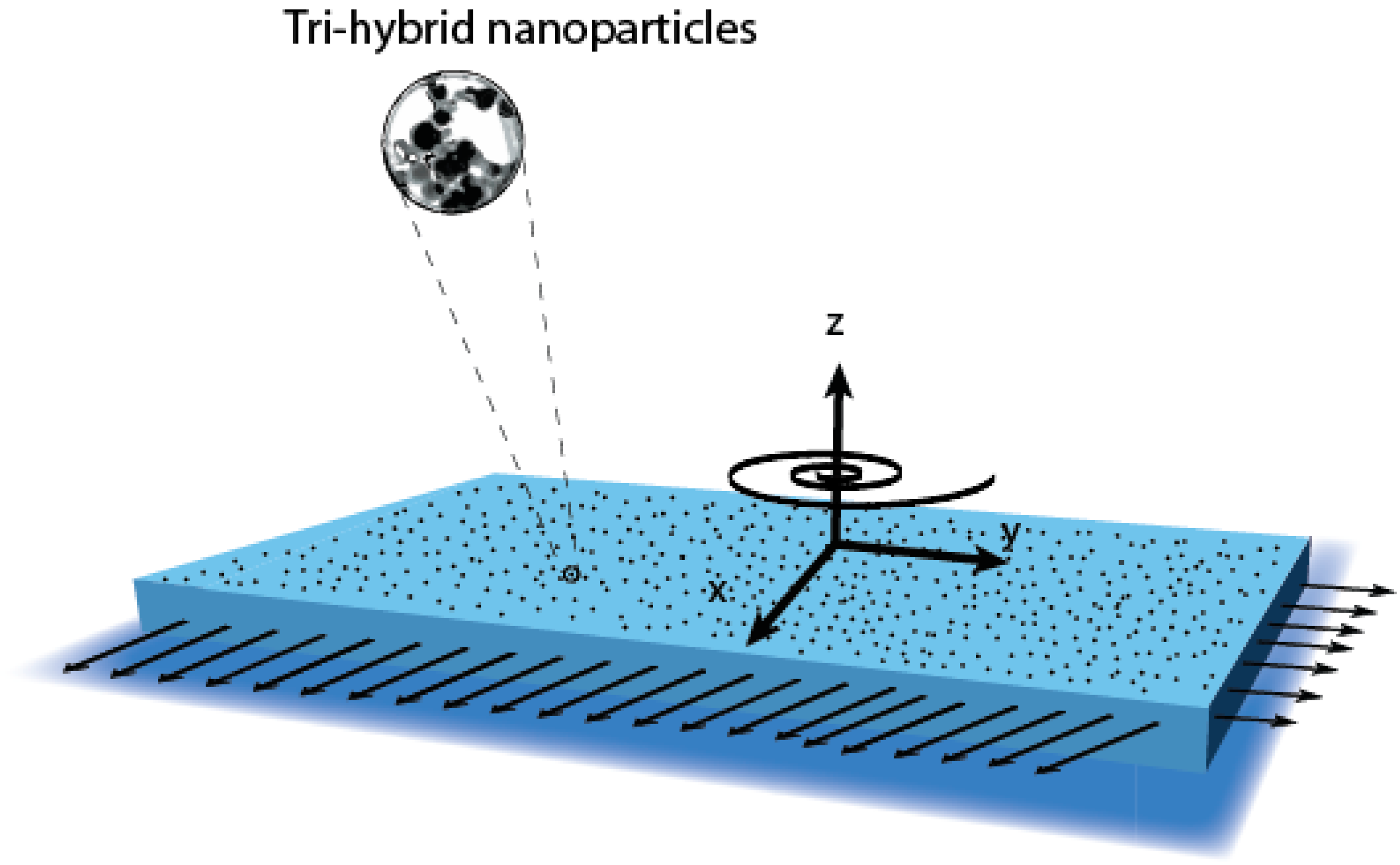
2. Statement of Developing Problem

Thermal features of a hyperbolic tangent martial towards a rotating frame are considered. The motion of tri-hybrid nanoparticles is induced by the movement of the wall and the rotation of the melting surface. The law related to Hall and ion-slip forces is incorporated to analyze the flow behavior in the presence of a Forchheimer porous medium. Heat characterizations occur due to Joule heating and viscous dissipation. A new theoretical scheme is implemented based on tri-hybrid nanoparticles. The composite of $A{l}_2{O}_3,Ti{O}_2$ and $Si{O}_2$ in $C_2{H}_6{O}_2$ is called tri-hybrid nanoparticles, while the composite relation among $A{l}_2{O}_3$ and $Si{O}_2$ is known as hybrid nanoparticles, and $Si{O}_2$ is nanofluid. A magnetic field is considered in the normal direction of surface. A continuity equation (mentioned in Equation (1)) for steady and incompressible flow is formulated in $x$-, $y$- and $z$-directions using boundary layer approximations and the law of conservation of mass. Momentum equations (mentioned in Equations (2) and (3)) are modeled, considering the Darcy–Forchheimer law and generalized Ohm’s law. An energy equation is derived using the Darcy–Forchheimer law, generalized Ohm’s law, Joule heating and viscous dissipation. The geometry of this model is shown in Figure 2.

A set of nonlinear partial differential equations (PDEs) is modeled under boundary layer approximations (BLAs) and assumptions, while the simplified PDEs [30,31] are

$$\frac{\partial \overline{u}}{\partial x}+\frac{\partial \overline{v}}{\partial y}+\frac{\partial \overline{w}}{\partial z}=0,$$

(3)

$$\begin{array}{c}\overline{u}\frac{\partial \overline{u}}{\partial x}+\overline{v}\frac{\partial \overline{u}}{\partial y}+\overline{w}\frac{\partial \overline{u}}{\partial z}=2\omega \overline{v}-\frac{{\nu }_{Thnf}}{k^{\ast }}{F}_s\overline{u}-\frac{F_s}{{\left(k^{\ast }\right)}^{\frac{1}{2}}}{\overline{u}}^2+{\nu }_{Thnf}\left(1-n\right)\frac{{\partial }^2\overline{u}}{\partial z^2}\\ +{\nu }_{Thnf}\sqrt{2}n\mathsf{\Gamma }\left(\frac{\partial \overline{u}}{\partial z}\right)\frac{{\partial }^2\overline{u}}{\partial z^2}+\frac{{\left(B_0\right)}^2{\sigma }_{Thnf}}{{\rho }_{Thnf\left[{\beta }_e^2+{\left(1+{\beta }_e{\beta }_i\right)}^2\right]}}\left[{\beta }_e\overline{v}-\left(1+{\beta }_e{\beta }_i\right)\overline{u}\right],\end{array}$$

(4)

$$\begin{gathered} \overline{u}\frac{\partial \overline{v}}{\partial x}+\overline{v}\frac{\partial \overline{v}}{\partial y}+\overline{w}\frac{\partial \overline{v}}{\partial z}=-2\omega \overline{u}-\frac{{\nu }_{Thnf}}{k^{\ast }}{F}_s\overline{v}-\frac{F_s}{{\left(k^{\ast }\right)}^{\frac{1}{2}}}{\overline{v}}^2+{\nu }_{Thnf}\left(1-n\right)\frac{{\partial }^2\overline{v}}{\partial z^2} \\ +\sqrt{2}n{\nu }_{Thnf}\mathsf{\Gamma }\left(\frac{\partial \overline{v}}{\partial z}\right)\frac{{\partial }^2\overline{v}}{\partial z^2}-\frac{{\left(B_0\right)}^2{\sigma }_{Thnf}}{{\rho }_{Thnf\left[{\beta }_e^2+{\left(1+{\beta }_e{\beta }_i\right)}^2\right]}}\left[{\beta }_e\overline{u}+\left(1+{\beta }_e{\beta }_i\right)\overline{v}\right], \end{gathered}$$

(5)

$$\begin{gathered} \overline{u}\frac{\partial \overline{T}}{\partial x}+\overline{v}\frac{\partial \overline{T}}{\partial y}+\overline{w}\frac{\partial \overline{T}}{\partial z}=\frac{K_{Thnf}}{{\left(\rho C_P\right)}_{Thnf}}\frac{{\partial }^2\overline{T}}{\partial z^2}+\frac{{\left(B_0\right)}^2{\sigma }_{Thnf}}{{\left(\rho C_P\right)}_{Thnf}\left[{\beta }_e^2+{\left(1+{\beta }_e{\beta }_i\right)}^2\right]}\left({\overline{u}}^2+{\overline{v}}^2\right) \\ +\frac{{\mu }_{Thnf}}{{\left(\rho C_P\right)}_{Thnf}}\left[\left(1-n\right)+\frac{n\mathsf{\Gamma }}{\sqrt{2}}{\left({\left(\frac{\partial \overline{u}}{\partial z}\right)}^2+{\left(\frac{\partial \overline{v}}{\partial z}\right)}^2\right)}^{\frac{1}{2}}\left\{{\left(\frac{\partial \overline{u}}{\partial z}\right)}^2+{\left(\frac{\partial \overline{v}}{\partial z}\right)}^2\right\}\right]. \end{gathered}$$

(6)

Here, space coordinates $\left(z,x,y\right)$, velocities ($\overline{w},\overline{v},\overline{w}$), kinematic viscosity ($\nu$), Hall number (${\beta }_e$), ion-slip number (${\beta }_i$), magnetic number ($B_0$), time constant number ($\mathsf{\Gamma }$), electrical conductivity ($\sigma$), fluid density ($\rho$), power law number ($n$), thermal conductivity ($K$), specific heat capacitance ($C_P$), fluid dynamic viscosity ($\mu$), permeability related to porous medium ($k_{\ast }$), inertia coefficient in view of porous medium ($F_s$) and tri-hybrid nanoparticles ($Thnf$) are captured above. A set of PDEs is formulated according to required boundary conditions, and boundary conditions (BCs) are modeled as

$$\begin{gathered} \overline{u}=Ax,\overline{v}=0,\overline{w}=0,\overline{T}=T_w,\mathrm{when}z=0, \\ \overline{u}\to 0,\overline{v}\to 0,\overline{T}\to T_{\infty },\mathrm{at}z\to \infty . \end{gathered}$$

(7)

Transformations of the current model are

$$\overline{u}=Ax{F}^{\prime },\overline{v}=AxG,\overline{w}=-F{\left(A{\nu }_F\right)}^{\frac{1}{2}},\xi ={\left(\frac{A}{{\nu }_f}\right)}^{\frac{1}{2}}z,\theta =\frac{\overline{T}-T_{\infty }}{T_w-T_{\infty }}.$$

(8)

Using transformations, a set of non-linear ordinary differential equations (ODEs) are obtained as

$$\begin{gathered} \left(1-m\right)F^{‴}+mWe{F}^{″}{F}^{‴}+\frac{{\nu }_f}{{\nu }_{Thnf}}\left[\left(F\right)F^{″}-F^{\prime }\left(F^{\prime }\right)\right]+\frac{{\nu }_f}{{\nu }_{Thnf}}2G\mathsf{\Omega } \\ +\frac{{\left(1-{\phi }_1\right)}^{2.5}{\left(1-{\phi }_3\right)}^{2.5}{M}^2{\left(1-{\phi }_2\right)}^{2.5}}{{\beta }_e^2+{\left(1+{\beta }_i{\beta }_e\right)}^2}\left[{\beta }_{e}G-\left(1+{\beta }_i{\beta }_e\right)F^{\prime }\right]-ϵF^{\prime }-\frac{{\nu }_f}{{\nu }_{Thnf}}{F}_r{F^{\prime }}^2=0, \end{gathered}$$

(9)

$$\begin{gathered} \left(1-m\right)G^{″}+mWe{G}^{\prime }{G}^{″}+\frac{{\nu }_f}{{\nu }_{Thnf}}\left[\left(F\right)G^{\prime }-F^{\prime }\left(G\right)\right]-2\frac{{\nu }_f}{{\nu }_{Thnf}}{F}^{\prime }\mathsf{\Omega } \\ -\frac{{\left(1-{\phi }_1\right)}^{2.5}{M}^2{\left(1-{\phi }_3\right)}^{2.5}{\left(1-{\phi }_2\right)}^{2.5}}{{\beta }_e^2+{\left(1+{\beta }_i{\beta }_e\right)}^2}\left[{\beta }_e{F}^{\prime }+\left(1+{\beta }_i{\beta }_e\right)G\right]-ϵG-\frac{{\nu }_f}{{\nu }_{Thnf}}{F}_r{G}^2=0, \end{gathered}$$

(10)

$$\begin{gathered} {\theta }^{″}+\frac{K_f}{K_{Thnf}}\frac{{\left(\rho C_P\right)}_{Thnf}}{{\left(\rho C_P\right)}_f}Pr{\theta }^{\prime }F+\frac{K_f}{K_{Thnf}}\frac{M^{2}PrEc}{\left[{\beta }_e^2+{\left(1+{\beta }_e{\beta }_i\right)}^2\right]}\left[{F^{\prime }}^2+G^2\right] \\ +\frac{{\left(1-{\phi }_2\right)}^{-2.5}{K}_f}{{\left(1-{\phi }_3\right)}^{2.5}{K}_{Thnf}}\frac{EcPr}{{\left(1-{\phi }_1\right)}^{2.5}}\left[{F^{″}}^2+{G^{\prime }}^2\right] \\ +\frac{{\left(1-{\phi }_2\right)}^{-2.5}{K}_f}{{\left(1-{\phi }_3\right)}^{2.5}{K}_{Thnf}}\frac{WeEcPr}{{\left(1-{\phi }_1\right)}^{2.5}}\left[{\left({F^{″}}^2+{G^{\prime }}^2\right)}^{1/2}\right]\left[{F^{″}}^2+{G^{\prime }}^2\right]=0. \end{gathered}$$

(11)

Dimensionless (boundary equations) BCs via variables and desired (boundary equations) BCs are defined as

$$F\left(0\right)=0,F^{\prime }\left(0\right)=1,F^{\prime }(\infty )=0,G\left(0\right)=0,\theta \left(0\right)=1,G^{\prime }\left(0\right)=0,\theta (\infty )=0.$$

(12)

Correlations among tri-hybrid nanoparticles, nanofluid and hybrid nanoparticles in view of the base fluid, ethylene glycol, are defined [17] as follows and the Thermal properties are listed in

Table 1. Thermal properties [32] of $A{l}_2{O}_3,Ti{O}_2,C_2{H}_6{O}_2$ and $Si{O}_2$.

	$\mathit{K} \text{(Thermal Conductivity)}$	$\mathit{\sigma } \text{(Electical Conductivity)}$	$\mathit{\rho } \text{(Desity)}$
$C_2{H}_6{O}_2$	0.253	$4.3\times {10}^{-5}$	1113.5
$A{l}_2{O}_3$	32.9	$5.96\times {10}^7$	6310
$Ti{O}_2$	8.953	$2.4\times {10}^6$	4250
$Si{O}_2$	1.4013	$3.5\times {10}^6$	2270

.

$${\rho }_{Thnf}=\left(1-{\phi }_1\right)\left\{\left(1-{\phi }_2\right)\left[\left(1-{\phi }_3\right){\rho }_f+{\phi }_3{\rho }_3\right]+{\phi }_2{\rho }_2\right\}+{\phi }_1{\rho }_1,$$

(13)

$$\begin{gathered} {\mu }_{Thnf}=\frac{{\mu }_f}{{\left(1-{\phi }_3\right)}^{2.5}{\left(1-{\phi }_2\right)}^{2.5}{\left(1-{\phi }_1\right)}^{2.5}},\frac{K_{hnf}}{K_{nf}}=\frac{K_2+2K_{nf}-2{\phi }_1\left(K_{nf}-K_1\right)}{K_1+2K_{nf}+{\phi }_1\left(K_{nf}-K_1\right)}, \\ \frac{K_{Thnf}}{K_{hnf}}=\frac{K_2+2K_{hnf}-2{\phi }_2\left(K_{hnf}-K_2\right)}{K_2+2K_{hnf}+{\phi }_2\left(K_{nf}-K_2\right)},\frac{K_{nf}}{K_f}=\frac{K_3+2K_f-2{\phi }_3\left(K_f-K_3\right)}{K_3+2K_f+{\phi }_3\left(K_f-K_3\right)}, \end{gathered}$$

(14)

$$\frac{{\sigma }_{Tnf}}{{\sigma }_{hnf}}=\frac{{\sigma }_1\left(1+2{\phi }_1\right)+{\phi }_{hnf}\left(1-2{\phi }_1\right)}{{\sigma }_1\left(1-{\phi }_1\right)+{\sigma }_{hnf}\left(1+{\phi }_1\right)},\frac{{\sigma }_{nf}}{{\sigma }_{nf}}=\frac{{\sigma }_2\left(1+2{\phi }_2\right)+{\phi }_{nf}\left(1-2{\phi }_2\right)}{{\sigma }_2\left(1-{\phi }_2\right)+{\sigma }_{nf}\left(1+{\phi }_2\right)},$$

(15)

$$\frac{{\sigma }_{nf}}{{\sigma }_f}=\frac{{\sigma }_3\left(1+2{\phi }_3\right)+{\phi }_f\left(1-2{\phi }_3\right)}{{\sigma }_3\left(1-{\phi }_3\right)+{\sigma }_f\left(1+{\phi }_3\right)}.$$

(16)

Here, volume fractions (${\phi }_1,{\phi }_3,{\phi }_2$), wall temperature ($T_w$), ambient temperature ($T_{\infty }$), naofluid ($nf$), base fluid ($f$), ethylene glycol ($C_2{H}_6{O}_2$), silicon dioxide ($Si{O}_2$), aluminum oxide ($A{l}_2{O}_3$) and titanium dioxide ($Ti{O}_2$) are defined above. The Weissenberg number ($We$), Prandtl number ($Pr$), magnetic number ($M^2$), Eckert number ($Ec$), rotation number ($\mathsf{\Omega }$), porosity number ($ϵ$) and Forchheimer number ($F_r$) are expressed below.

$$\begin{gathered} We=\frac{xa\sqrt{a\mathsf{\Gamma }}}{\sqrt{{\nu }_f}},\mathsf{\Omega }\left(=\frac{\omega }{a}\right),Pr=\frac{{\left(C_P\right)}_f{\mu }_f}{K_f},F_r\left(=\frac{F_{s}x}{{\left(k_{\ast }\right)}^{1/2}}\right), \\ ϵ\left(=\frac{{\nu }_f{F}_s}{a}\right),Ec\left(=\frac{{\left(U_w\right)}^2}{{\left(C_P\right)}_f{\left(T_w-T_{\infty }\right)}^2}\right),M^2\left(=\frac{B_0^2{\sigma }_{Thnf}}{a{\rho }_f}\right). \end{gathered}$$

Skin friction coefficients in the presence of a hyperbolic tangent martial is modeled as

$$C_F=\frac{{{\tau }_{zx}|}_{z=0}}{{\left(U_w\right)}^2{\rho }_{Thnf}},$$

(17)

$${\left(Re\right)}^{1/2}{C}_F=\frac{1}{{\left(1-{\phi }_2\right)}^{2.5}{\left(1-{\phi }_3\right)}^{2.5}{\left(1-{\phi }_1\right)}^{2.5}}\left[\left(1-m\right)F^{″}\left(0\right)+\frac{m}{2}We{F}^{″}{\left(0\right)}^2\right],$$

(18)

$$C_G=\frac{{{\tau }_{zy}|}_{z=0}}{{\left(U_w\right)}^2{\rho }_{Thnf}},$$

(19)

$${\left(Re\right)}^{1/2}{C}_G=\frac{1}{{\left(1-{\phi }_2\right)}^{2.5}{\left(1-{\phi }_3\right)}^{2.5}{\left(1-{\phi }_1\right)}^{2.5}}\left[\left(1-m\right)G^{\prime }\left(0\right)+\frac{m}{2}We{G}^{\prime }{\left(0\right)}^2\right].$$

(20)

The Nusselt number is a dimensionless parameter. It is noticed that the Nusselt number is the ratio of convective heat transfer and conductive heat transfer. From a mathematical point of view, the Nusselt number is defined as

$$Nu=\frac{x{Q}_w}{\left(T_w-T_{\infty }\right)K_f}.$$

(21)

The rate of heat transfer, called the temperature gradient, is

$${\left(Re\right)}^{-1/2}Nu=-\frac{K_{Thnf}}{K_f}{\theta }^{\prime }\left(0\right),$$

(22)

3. Numerical Approach

It is challenging for mathematicians and scientists to derive the exact solution of differential equations (DEs). Solutions related to some of the DEs are handled easily, but some higher order (nonlinear) problems are not as easily tackled due to the complexities of DEs. Various numerical methods are used to find solutions to such problems. The Keller box method, shooting method and RK method are numerical methods with numerous advantages. However, some limitations exist, such as stability and convergence of problems. There is agreement that the finite element approach [26,29] is the best technique to solve problems. The finite element method has a great ability to handle complex geometries, along with various types of boundary conditions (BCs). A strong approach, called the finite element approach, is imposed to obtain a numerical solution of formulated ODEs associated with BCs. The steps related to the discussion of the finite element approach (FEA) are discussed below.

Step-I: Residuals are made by adjusting all terms in one place within BCs. Equations (7)–(9) are known as strong form, while the conversion from strong form into weak form is conducted via the weighted residual method. The weighted residuals of the present problem are:

$${{\displaystyle \int }}_{{\eta }_e}^{{\eta }_{e+1}}{W}_1\left[F^{\prime }-T\right]d\eta =0,$$

(23)

$${{\displaystyle \int }}_{{\eta }_e}^{{\eta }_{e+1}}{W}_2\left[\begin{array}{c}\left(1-m\right)T^{″}+mWe{T}^{\prime }{T}^{″}+\frac{{\nu }_f}{{\nu }_{Thnf}}\left[\left(F\right)T^{\prime }-T\left(T\right)\right]\\ +\frac{{\left(1-{\varphi }_1\right)}^{2.5}{\left(1-{\varphi }_3\right)}^{2.5}{M}^2{\left(1-{\varphi }_2\right)}^{2.5}}{{\beta }_e^2+{\left(1+{\beta }_i{\beta }_e\right)}^2}\left[{\beta }_{e}G-\left(1+{\beta }_i{\beta }_e\right)T\right]\\ +\frac{{\nu }_f}{{\nu }_{Thnf}}2G\Omega -ϵT-\frac{{\nu }_f}{{\nu }_{Thnf}}{F}_r{T}^2\end{array}\right]d\eta =0,$$

(24)

$${{\displaystyle \int }}_{{\eta }_e}^{{\eta }_{e+1}}{W}_3\left[\begin{array}{c}\left(1-m\right)G^{″}+mWe{G}^{\prime }{G}^{″}+\frac{{\nu }_f}{{\nu }_{Thnf}}\left[\left(F\right)G^{\prime }-T\left(G\right)\right]-2\frac{{\nu }_f}{{\nu }_{Thnf}}T\Omega \\ -\frac{{\left(1-{\varphi }_1\right)}^{2.5}{M}^2{\left(1-{\varphi }_3\right)}^{2.5}{\left(1-{\varphi }_2\right)}^{2.5}}{{\beta }_e^2+{\left(1+{\beta }_i{\beta }_e\right)}^2}\left[{\beta }_{e}T+\left(1+{\beta }_i{\beta }_e\right)G\right]\\ -ϵG-\frac{{\nu }_f}{{\nu }_{Thnf}}{F}_r{G}^2\end{array}\right]d\eta =0,$$

(25)

$${\int }_{{\eta }_e}^{{\eta }_{e+1}}{W}_4\left[\begin{array}{c}{\theta }^{″}+\frac{K_f}{K_{\mathit{Thnf}}}\frac{{\left(\rho C_P\right)}_{Thnf}}{{\left(\rho C_P\right)}_f}Pr{\theta }^{\prime }F+\frac{K_f}{K_{\mathit{Thnf}}}\frac{M^{2}PrEc}{\left[{\beta }_e^2+{\left(1+{\beta }_e{\beta }_i\right)}^2\right]}\left[T^2+G^2\right]\\ +\frac{{\left(1-{\varphi }_2\right)}^{-2.5}{K}_f}{{\left(1-{\varphi }_3\right)}^{2.5}{K}_{Thnf}}\frac{EcPr}{{\left(1-{\varphi }_1\right)}^{2.5}}\left[{T^{\prime }}^2+{G^{\prime }}^2\right]\\ +\frac{{\left(1-{\varphi }_2\right)}^{-2.5}{K}_f}{{\left(1-{\varphi }_3\right)}^{2.5}{K}_{Thnf}}\frac{WeEcPr}{{\left(1-{\varphi }_1\right)}^{2.5}}\left[{\left({T^{\prime }}^2+{G^{\prime }}^2\right)}^{1/2}\right]\left[{T^{\prime }}^2+{G^{\prime }}^2\right]\end{array}\right]d\eta =0,$$

(26)

where $W_1,W_2,W_3$ and $W_4$ are weight functions.

Step-II: An approach related to the Galerkin finite element scheme is implemented to make weak forms in terms of the shape functions.

Step-III: An assembly approach is utilized for the development of the stiffness element, and the assembly approach is performed via the assembly procedure of the finite element approach (FEA). Stiffness matrices are derived as

$$K_{ij}^{11}={{\displaystyle \int }}_{{\eta }_e}^{{\eta }_{e+1}}{\psi }_i\left(\frac{d{\psi }_j}{d\eta }\right)d\eta ,K_{ij}^{12}=-{{\displaystyle \int }}_{{\eta }_e}^{{\eta }_{e+1}}{\psi }_i{\psi }_{J}d\eta ,K_{ij}^{13}=0,K_{ij}^{14}=0,$$

(27)

$$K_{ij}^{22}={\int }_{{\eta }_e}^{{\eta }_{e+1}}\left[\begin{array}{c}-(1-m)\frac{d{\psi }_j}{d\eta }\frac{d{\psi }_i}{d\eta }-mWe\overline{T^{\prime }}\frac{d{\psi }_j}{d\eta }\frac{d{\psi }_i}{d\eta }+\frac{v_f}{v_{\mathit{Thnf}}}\overline{F}{\psi }_i\frac{d{\psi }_j}{d\eta }\\ -\frac{v_f}{v_{\mathrm{Thnf}}}\overline{T}{\psi }_i{\psi }_j+\frac{\left(1+{\beta }_i{\beta }_e\right){\left(1-{\varphi }_1\right)}^{2.5}{\left(1-{\varphi }_3\right)}^{2.5}{M}^2{\left(1-{\varphi }_2\right)}^{2.5}}{{\beta }_e^2+{\left(1+{\beta }_i{\beta }_e\right)}^2}{\psi }_i{\psi }_j\\ -ϵ{\psi }_i{\psi }_j-\frac{v_f}{v_{\mathrm{Thnf}}}{F}_r\overline{T}{\psi }_i{\psi }_j\end{array}\right]d\eta ,$$

(28)

$$K_{ij}^{23}={{\displaystyle \int }}_{{\eta }_e}^{{\eta }_{e+1}}\left[\frac{{\nu }_f}{{\nu }_{Thnf}}2\mathsf{\Omega }{\psi }_i{\psi }_j+\frac{{\left(1-{\varphi }_1\right)}^{2.5}{\left(1-{\varphi }_3\right)}^{2.5}{M}^2{\left(1-{\varphi }_2\right)}^{2.5}}{{\beta }_e^2+{\left(1+{\beta }_i{\beta }_e\right)}^2}{\beta }_e{\psi }_i{\psi }_j\right]d\eta ,$$

(29)

$$K_{ij}^{24}=0,b_i^1=0,b_i^2=0,K_{ij}^{31}=0,K_{ij}^{34}=0,b_i^1=0,K_{ij}^{21}=0,$$

(30)

$$K_{ij}^{33}={\int }_{{\eta }_e}^{{\eta }_{e+1}}\left[\begin{array}{c}-(1-m)\frac{d{\psi }_j}{d\eta }\frac{d{\psi }_i}{d\eta }-mWe\overline{G^{\prime }}\frac{d{\psi }_j}{d\eta }\frac{d{\psi }_i}{d\eta }-\frac{v_f}{v_{Thnf}}\overline{F}\frac{d{\psi }_j}{d\eta }{\psi }_i-\frac{{\psi }_j{\psi }_i{v}_f}{v_{Thnf}}\overline{T}\hfill \\ \frac{{\left(1-{\varphi }_1\right)}^{2.5}{M}^2{\left(1-{\varphi }_3\right)}^{2.5}{\left(1-{\varphi }_2\right)}^{2.5}}{{\beta }_e^2+{\left(1+{\beta }_i{\beta }_e\right)}^2{\left(1+{\beta }_i{\beta }_e\right)}^{-1}}{\psi }_j{\psi }_i-ϵ{\psi }_j{\psi }_i-\frac{{\psi }_j{\psi }_i{F}_r{v}_f}{v_{Thnf}}\overline{G}\hfill \end{array}\right]d\eta ,$$

(31)

$$K_{ij}^{32}={{\displaystyle \int }}_{{\eta }_e}^{{\eta }_{e+1}}\left[-2\frac{{\nu }_f}{{\nu }_{Thnf}}\mathsf{\Omega }{\psi }_j{\psi }_i-\frac{{\left(1-{\varphi }_1\right)}^{2.5}{M}^2{\left(1-{\varphi }_3\right)}^{2.5}{\left(1-{\varphi }_2\right)}^{2.5}}{{\beta }_e^2+{\left(1+{\beta }_i{\beta }_e\right)}^2}{\beta }_e{\psi }_j{\psi }_i\right]d\eta ,$$

(32)

$$K_{ij}^{44}={{\displaystyle \int }}_{{\eta }_e}^{{\eta }_{e+1}}\left[-\frac{d{\psi }_j}{d\eta }\frac{d{\psi }_i}{d\eta }+\frac{K_f}{K_{Thnf}}\frac{{\left(\rho C_P\right)}_{Thnf}}{{\left(\rho C_P\right)}_f}Pr\overline{F}\frac{d{\psi }_j}{d\eta }{\psi }_i\right]d\eta ,$$

(33)

$$K_{ij}^{42}={{\displaystyle \int }}_{{\eta }_e}^{{\eta }_{e+1}}\left[\begin{array}{c}\frac{K_f}{K_{Thnf}}\frac{M^{2}PrEc}{\left[{\beta }_e^2+{\left(1+{\beta }_e{\beta }_i\right)}^2\right]}\overline{T}\frac{d{\psi }_j}{d\eta }{\psi }_i\\ +\frac{{\left(1-{\varphi }_2\right)}^{-2.5}{K}_f}{{\left(1-{\varphi }_3\right)}^{2.5}{K}_{Thnf}}\frac{EcPr}{{\left(1-{\varphi }_1\right)}^{2.5}}\overline{T^{\prime }}\left({\psi }_i\frac{d{\psi }_j}{d\eta }\right)\end{array}\right]d\eta ,b_i^4=0,$$

(34)

$$K_{ij}^{43}={{\displaystyle \int }}_{{\eta }_e}^{{\eta }_{e+1}}\left[\begin{array}{c}\frac{K_f}{K_{Thnf}}\frac{M^{2}PrEc}{\left[{\beta }_e^2+{\left(1+{\beta }_e{\beta }_i\right)}^2\right]}\overline{G}{\psi }_i{\psi }_j\\ +\frac{{\left(1-{\varphi }_2\right)}^{-2.5}{K}_f}{{\left(1-{\varphi }_3\right)}^{2.5}{K}_{Thnf}}\frac{EcPr}{{\left(1-{\varphi }_1\right)}^{2.5}}\overline{T^{\prime }}\left(\frac{d{\psi }_j}{d\eta }{\psi }_i\right)\end{array}\right]d\eta ,K_{ij}^{41}=0,$$

(35)

Step-IV: A Picard linearization approach provides a transformed algebraic system (linear equations).

Step-V: Finally, a system of linear algebraic equations is numerically solved within computational tolerance (${10}^{-5}$). The stopping condition is listed below.

$$\left|\frac{{\delta }_{i+1}-{\delta }_i}{{\delta }^i}\right|<{10}^{-5}.$$

(36)

Step-VI:

Table 2. Mesh-free investigation of temperature and velocities within 300 elements when $m=0.3,We=3,\mathsf{\Omega }=2.0,M^2=0.3,{\beta }_e=0.5,{\beta }_i=0.7,ϵ=0.01,F_r=2.5,Pr=204,Ec=0.34,{\phi }_2=0.0075,{\phi }_1=0.002,{\phi }_3=0.005$.

Elements	${\mathit{F}}^{\prime }\left(\frac{{\mathit{\eta }}_{\mathit{m}\mathit{a}\mathit{x}}}{2}\right)$	$\mathit{G}\left(\frac{{\mathit{\eta }}_{\mathit{m}\mathit{a}\mathit{x}}}{2}\right)$	$\mathit{\theta }\left(\frac{{\mathit{\eta }}_{\mathit{m}\mathit{a}\mathit{x}}}{2}\right)$
30	1.111381874	0.1033029114	0.5394657370
60	1.099801938	0.09383147162	0.5228689118
90	1.095986356	0.09090534841	0.5173330148
120	1.094092658	0.08948371769	0.5145656516
150	0.092961517	0.5129036217	0.08864385101
180	0.092212214	0.08808914037	0.5117970027
210	0.091677016	0.5110058672	0.08769570089
240	0.091275719	0.5104110691	0.08740183266
270	0.090964277	0.08717415891	0.5099497350
300	0.090715774	0.08799298080	0.5099823696

demonstrates the study of the mesh-free investigation.

Step-VII: 300 elements are required to obtain convergence analysis.

4. Graphical Outcomes and Discussion

Ternary hybrid nanoparticles are inserted into the motion of the fluid particles in the presence of ion-slip and Hall currents towards a 3D-stretching heated surface. The theory of Darcy–Forchheimer is carried out in the present analysis. Viscous dissipation and Joule heating are considered. The numerical results and graphical investigations are simulated by FEM. The details and outcomes of the present analysis are discussed below.

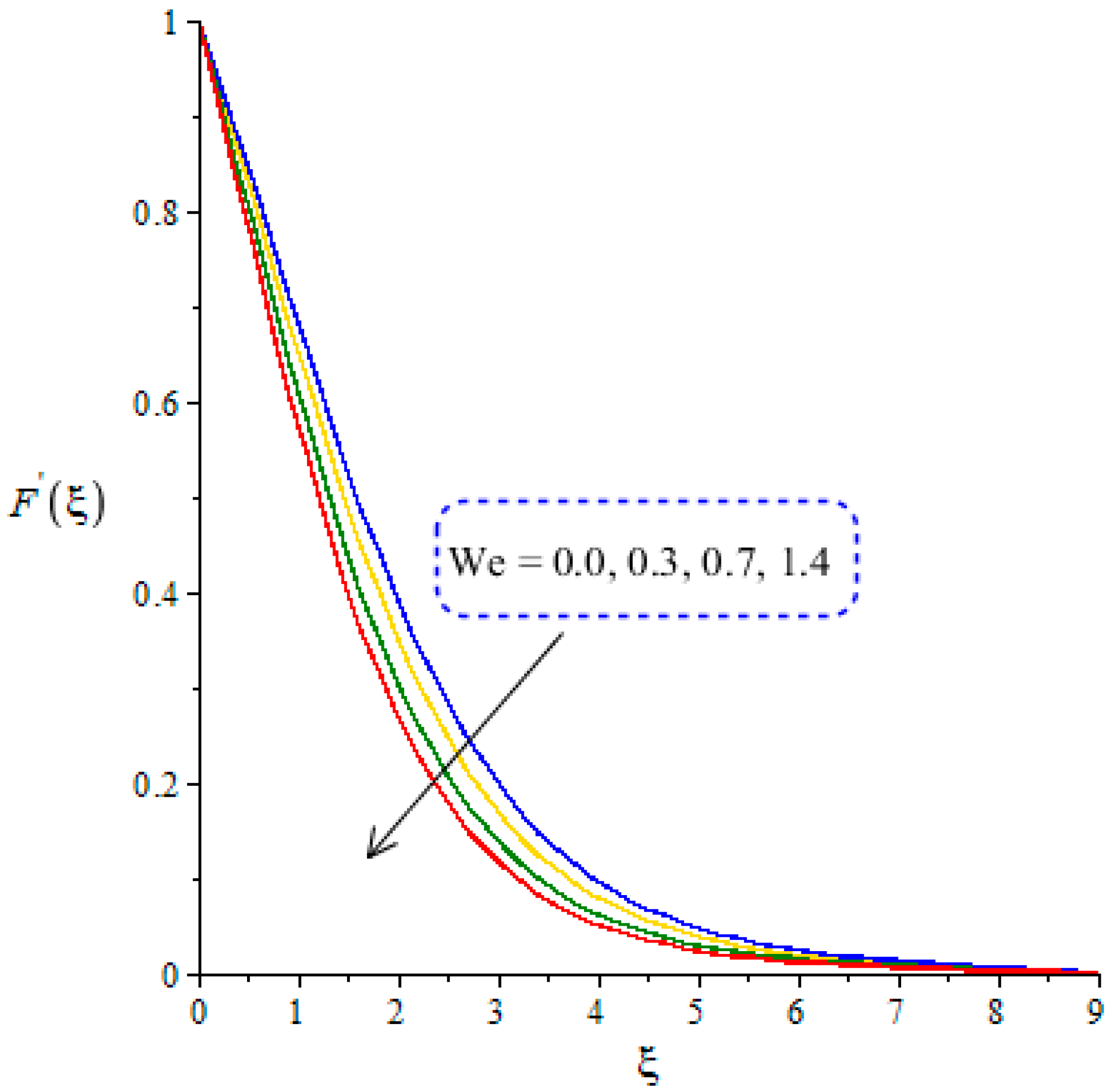
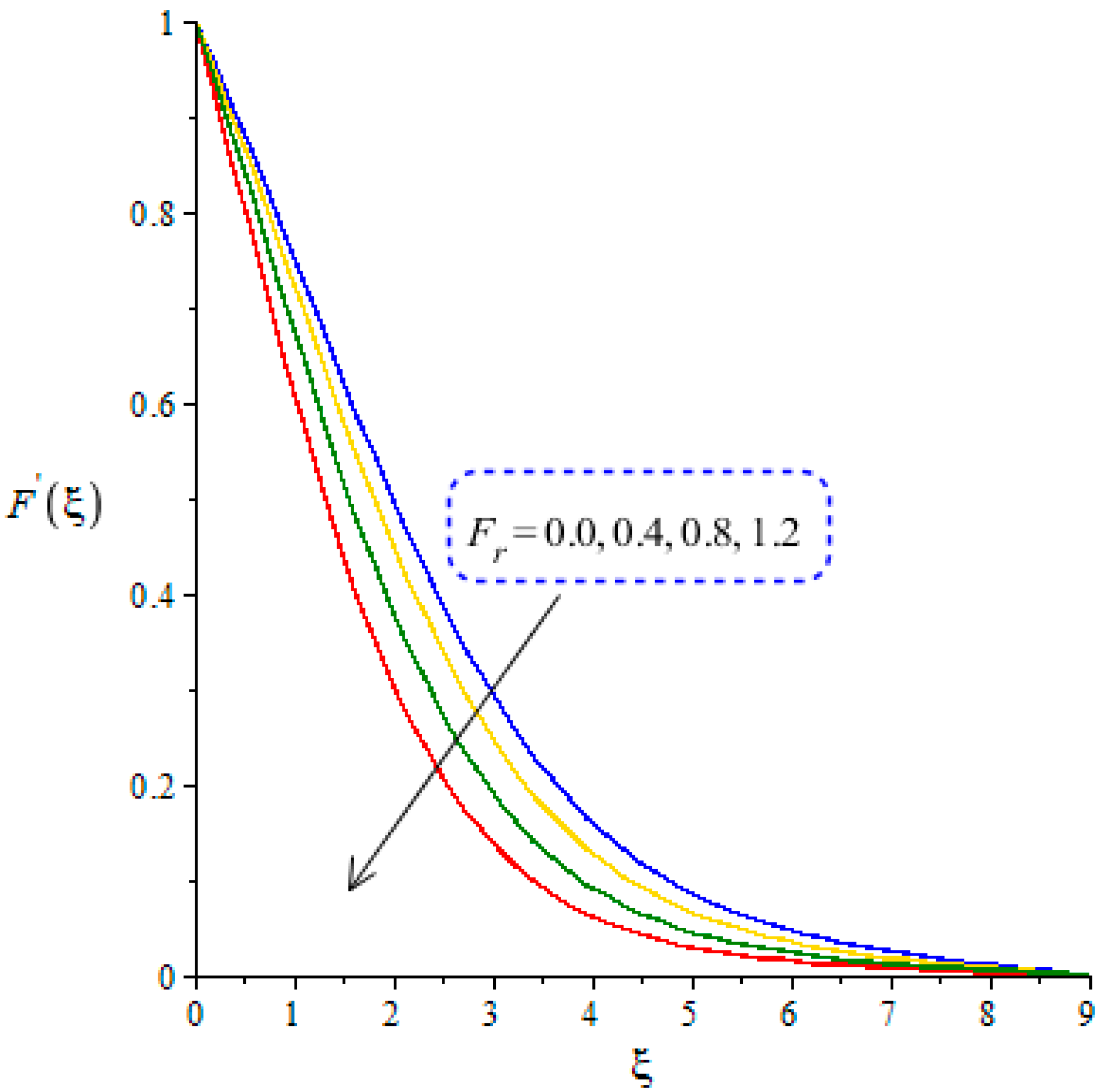
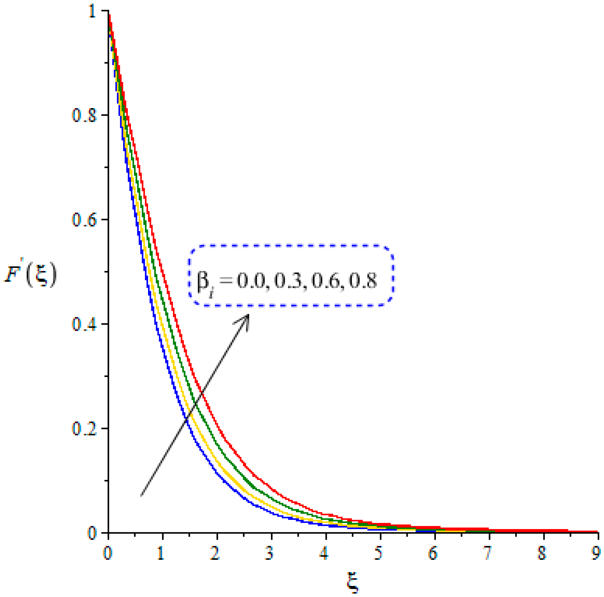
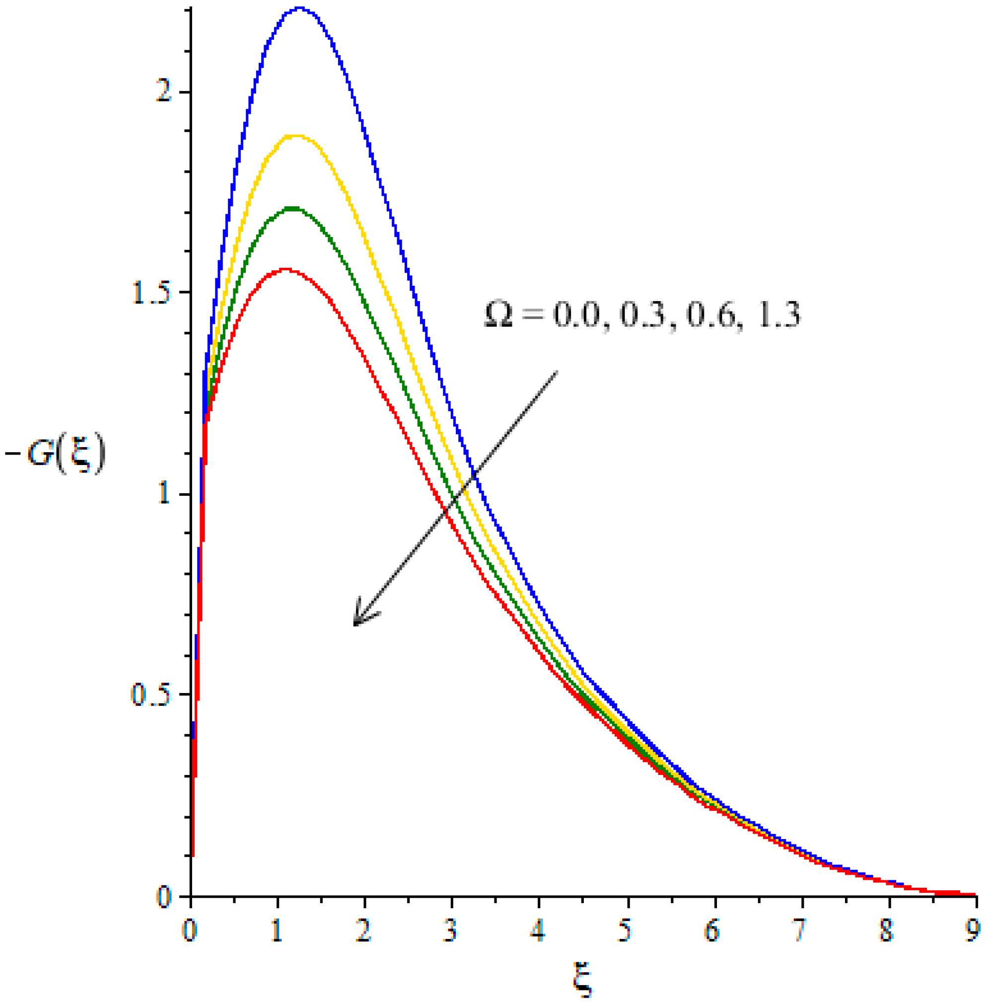
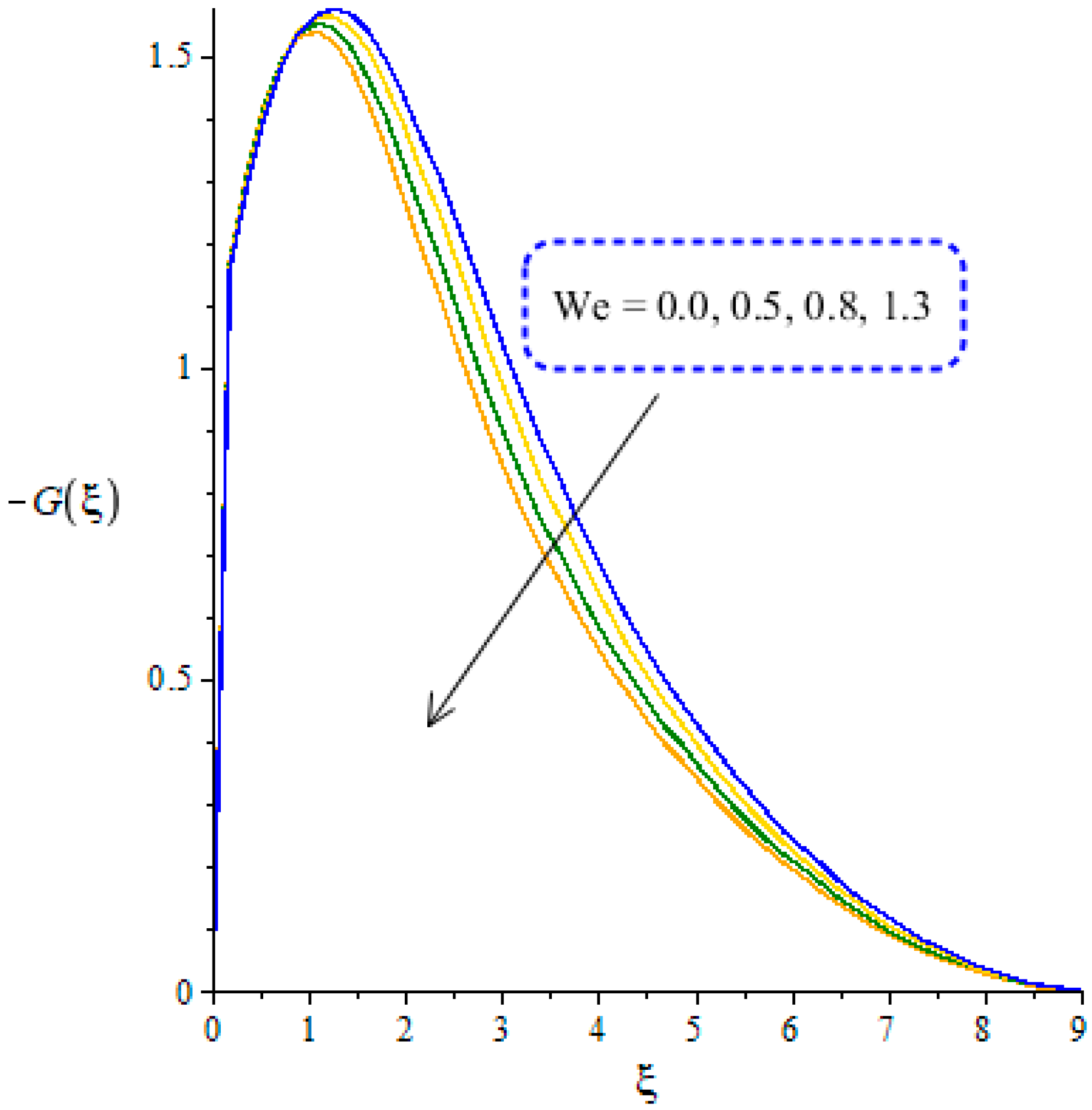
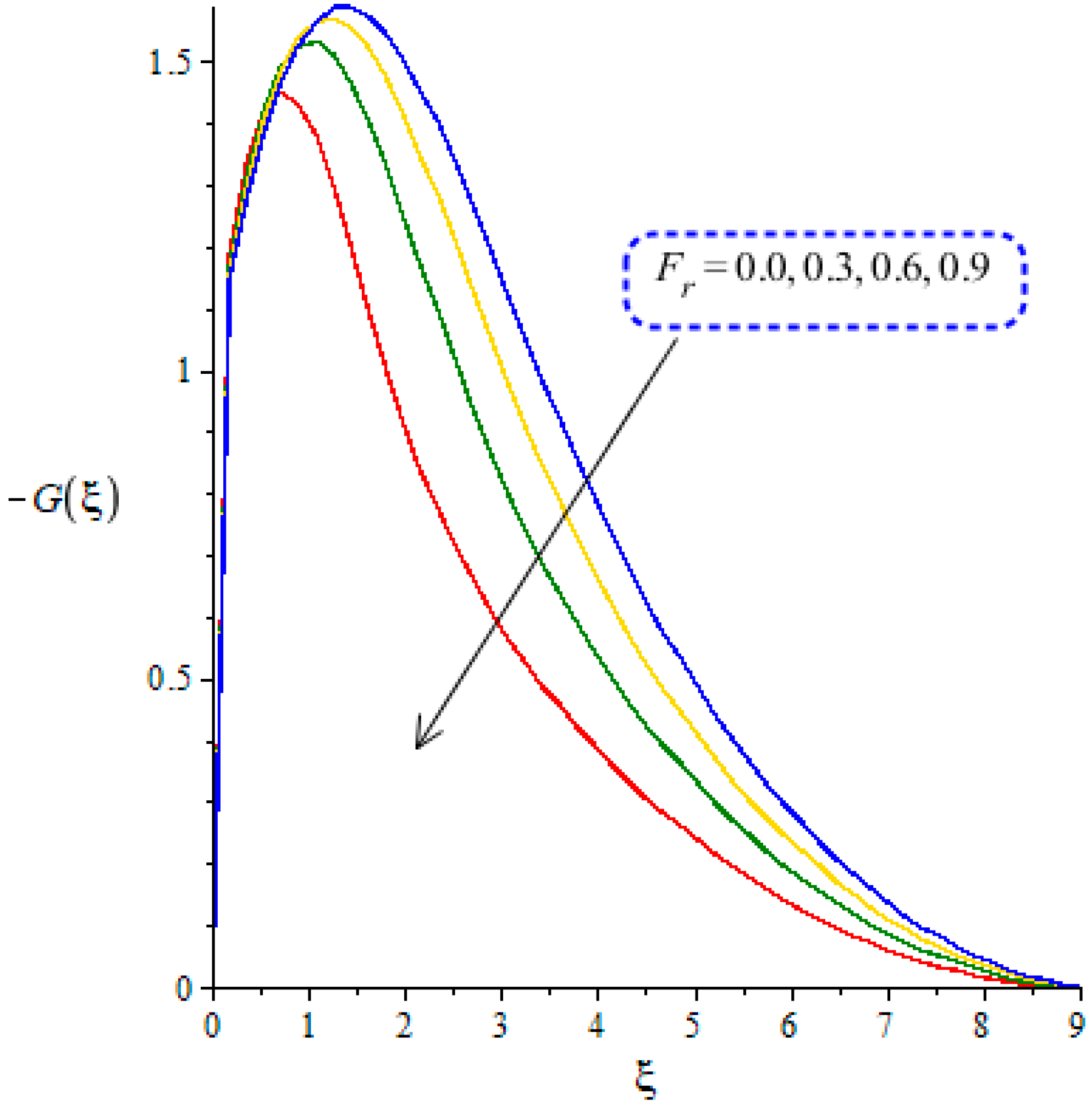
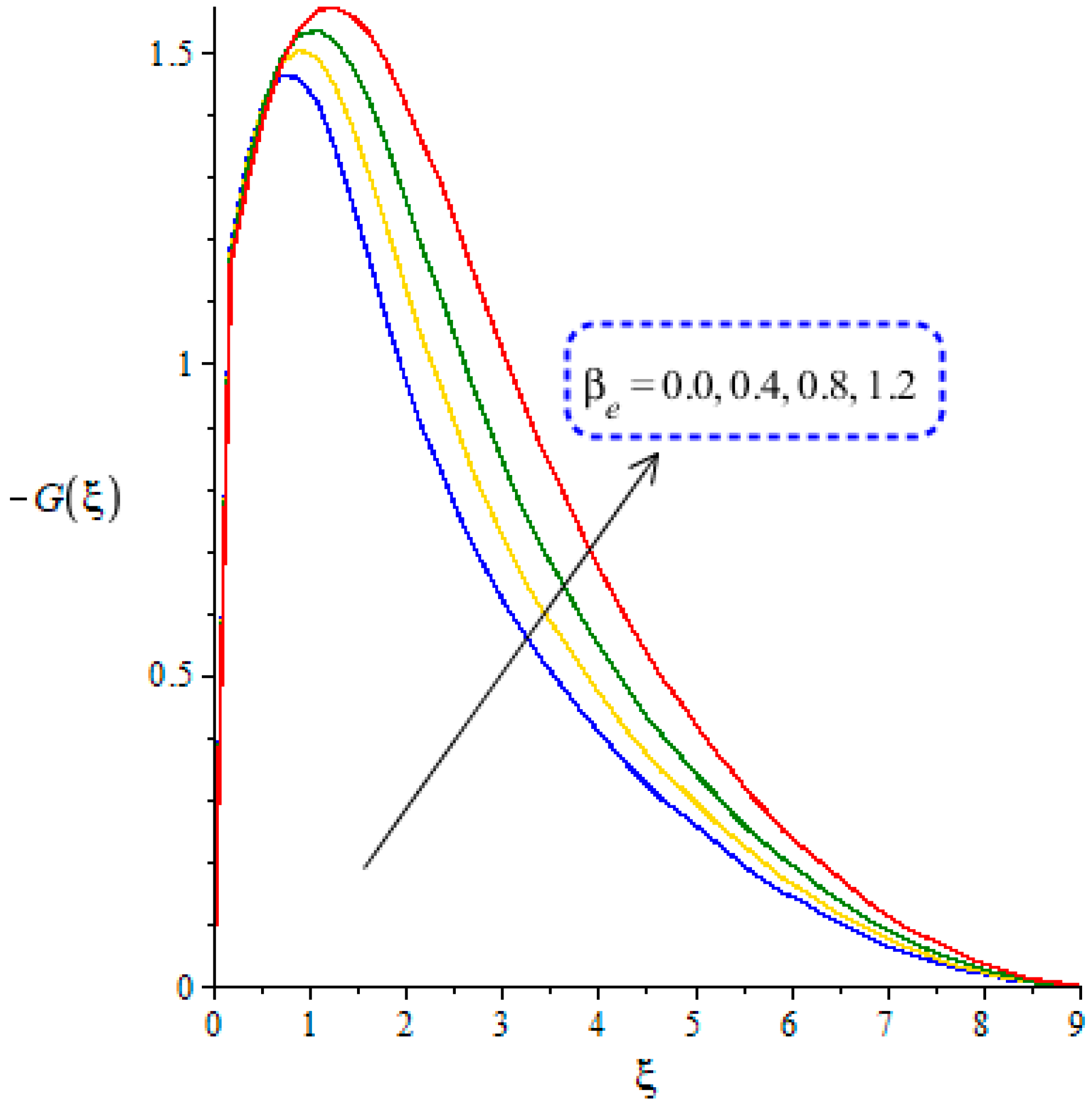
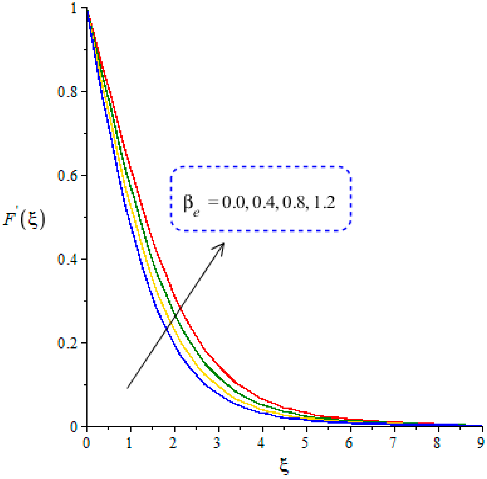
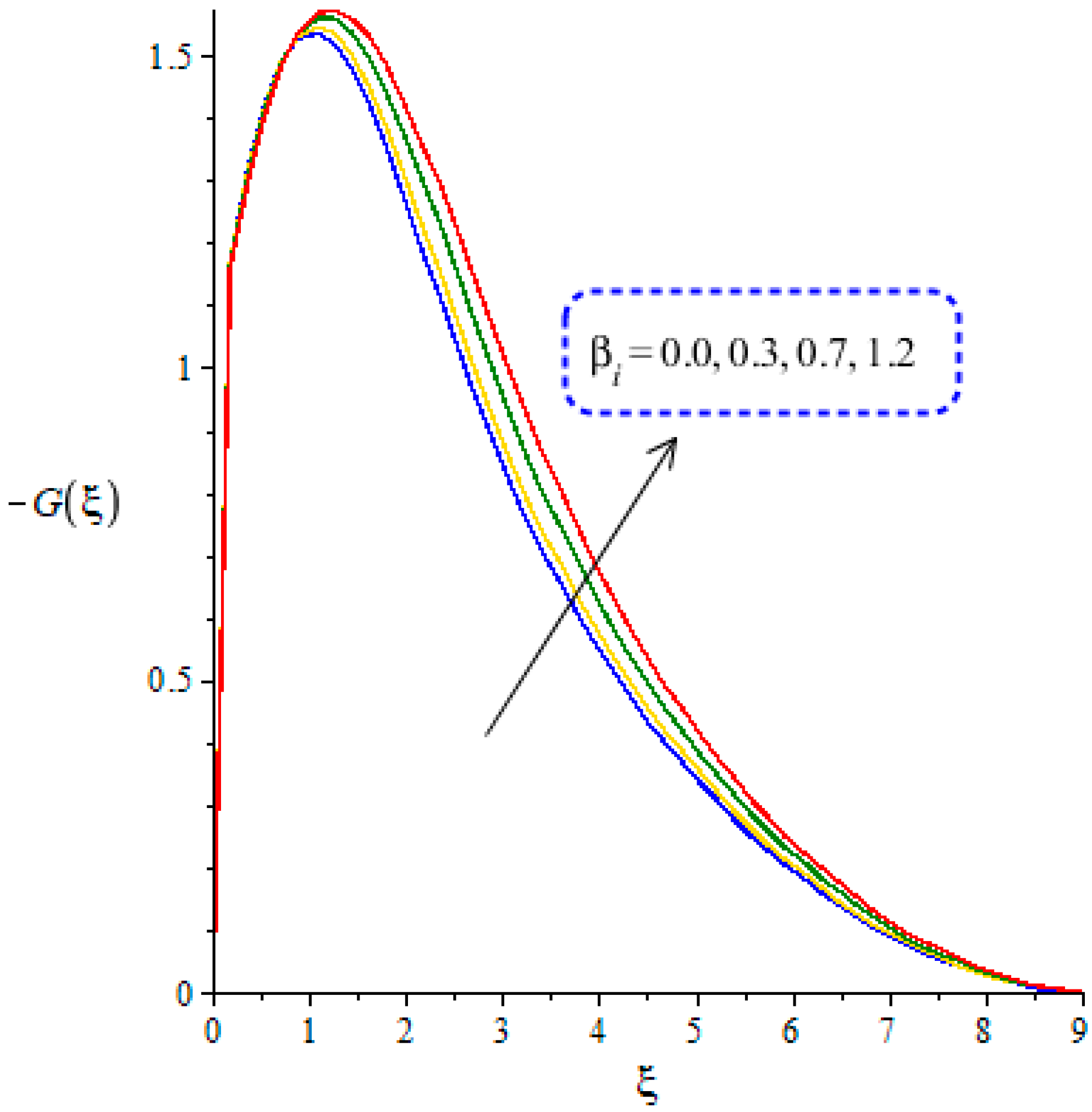
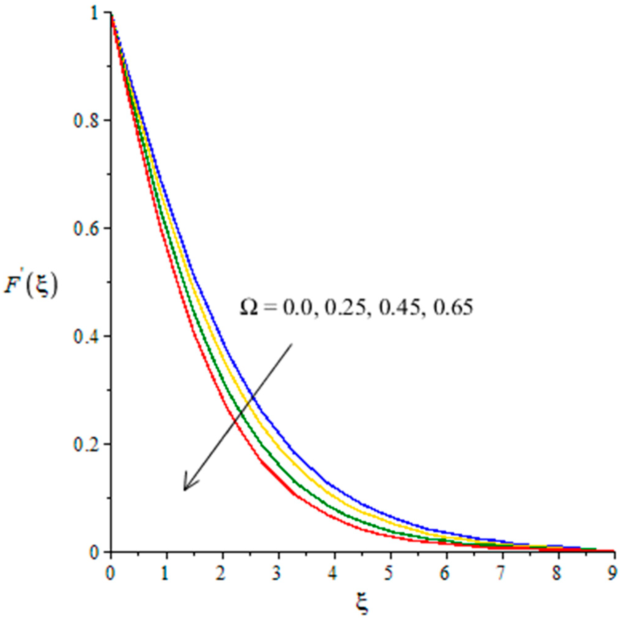
4.1. Outcomes of Velocity Profiles versus Parameters

The distribution of motion into fluid particles is analyzed versus the variation of the Weissenebrg number, ion-slip number, Hall number and Forchheimer number. Figure 3, Figure 4, Figure 5, Figure 6, Figure 7, Figure 8, Figure 9, Figure 10, Figure 11 and Figure 12 are plotted to show the distribution of motion (for vertical and horizontal velocities) into fluid particles. Figure 3 and Figure 4 show the influence of $We$ on the motion of fluid particles (for vertical and horizontal velocities). The motion into nanoparticles is reduced when $We$ is increased. It is deduced that the existence of $We$ is based on a hyperbolic tangent material in dimensionless momentum equations. Moreover, a decline in motion happened due to an inverse relation of $We$ versus the viscous force. Therefore, more viscosity is produced in the motion of fluid particles when $We$ is increased. Motion for the appearance of $We$ is higher than motion for the disappearance of $We$. Vertical and horizontal velocities are boosted when $We$ is enhanced. Physically, $We$ is the ratio among elastic force and viscous force, while fluid becomes more viscous when $We$ is increased. Hence, the viscosity of fluid particles becomes thicker due to the retardation of force. Thickness associated to the boundary layers is reduced using higher values of $We$. The influence of $F_r$ is visualized in the motion of fluid particles (for vertical and horizontal motions), and this impact is addressed in Figure 5 and Figure 6. Velocity curves are reduced versus variation in $F_r.$ Higher values of $F_r$ increase the thickness of the motion of the fluid particles. It is revealed that the parameter related to $F_r$ is modeled due to the Forchheimer theory, and the Darcy–Forchheimer flow has a nonlinear relationship against the flow of fluid. A retardation force is visualized when the Forchheimer flow is established. Moreover, $F_r$ is associated with the porosity of surfaces. The flow slows down due to the porosity of the surface in the $y$-and $x$-directions. The role of the Hall number (${\beta }_e$) is shown in Figure 7 and Figure 8 (for vertical and horizontal velocities). The motion into tri-hybrid nano-structures is boosted when the Hall number is enhanced. The Hall number exists because of the generalized Ohm’s theory, and the Hall number occurs in momentum and energy equations. Moreover, a direct relationship is tabulated among the Hall number and flow distribution. The Lorentz force is upgraded when the Hall number is boosted. Therefore, a higher Lorentz force introduces the argument of the motion of fluid particles. Physically, this occurs to manufacture more speed of fluid particles. Figure 9 and Figure 10 (for vertical and horizontal velocities) plot the relationship between fluid particles and the ion-slip number (${\beta }_i$). The law related to the generalized Ohm’s law is used in the motion of particles, which establishes the ion-slip number (${\beta }_i$). The thinning layers are produced when the ion-slip number (${\beta }_i$) is increased due to an inverse relationship between the Lorentz force and flow distribution. Moreover, the flow distribution for ${\beta }_i=0$ is higher, as compared to ${\beta }_i\ne 0$. Both ${\beta }_i$ and ${\beta }_e$ appear in the denominator (in momentum equations). Therefore, an inverse proportional relationship is captured among velocities and (${\beta }_i$ and ${\beta }_e$). The thickness of the momentum boundary layers declined but increased in ${\beta }_i$ and ${\beta }_e$. Figure 11 and Figure 12 reveal the role of velocity curves in $x$- and $y$-directions against the variation in $\mathsf{\Omega }$. It is estimated that the velocity curves are reduced when $\mathsf{\Omega }$ is increased, including the influence of tri-hybrid nanoparticles. The parameter associated with $\mathsf{\Omega }$ is generated due to the appearance of the rotating surface. Therefore, the role of the rotating frame, brings declination into the motion of fluid particles in both horizontal and vertical directions.

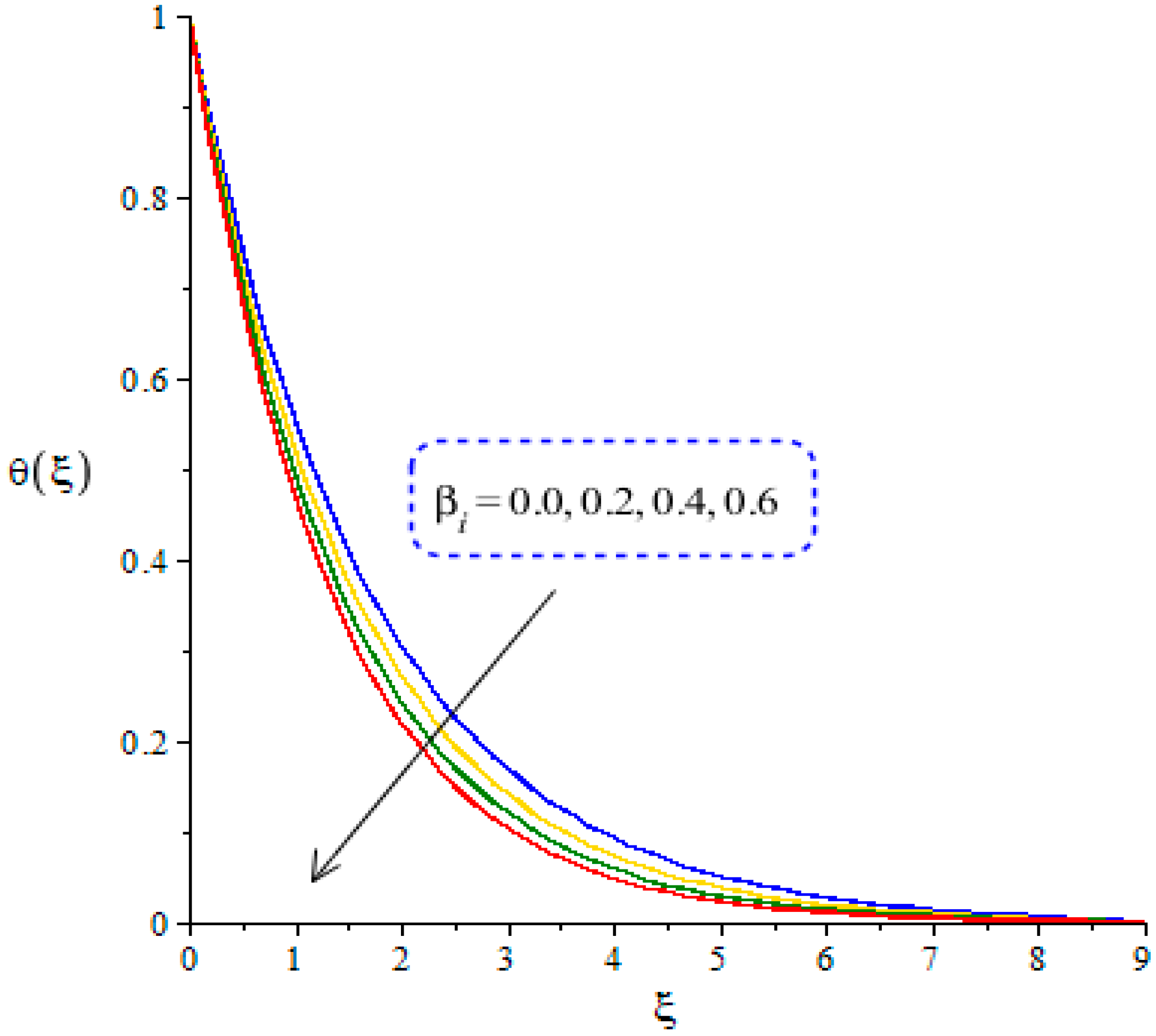
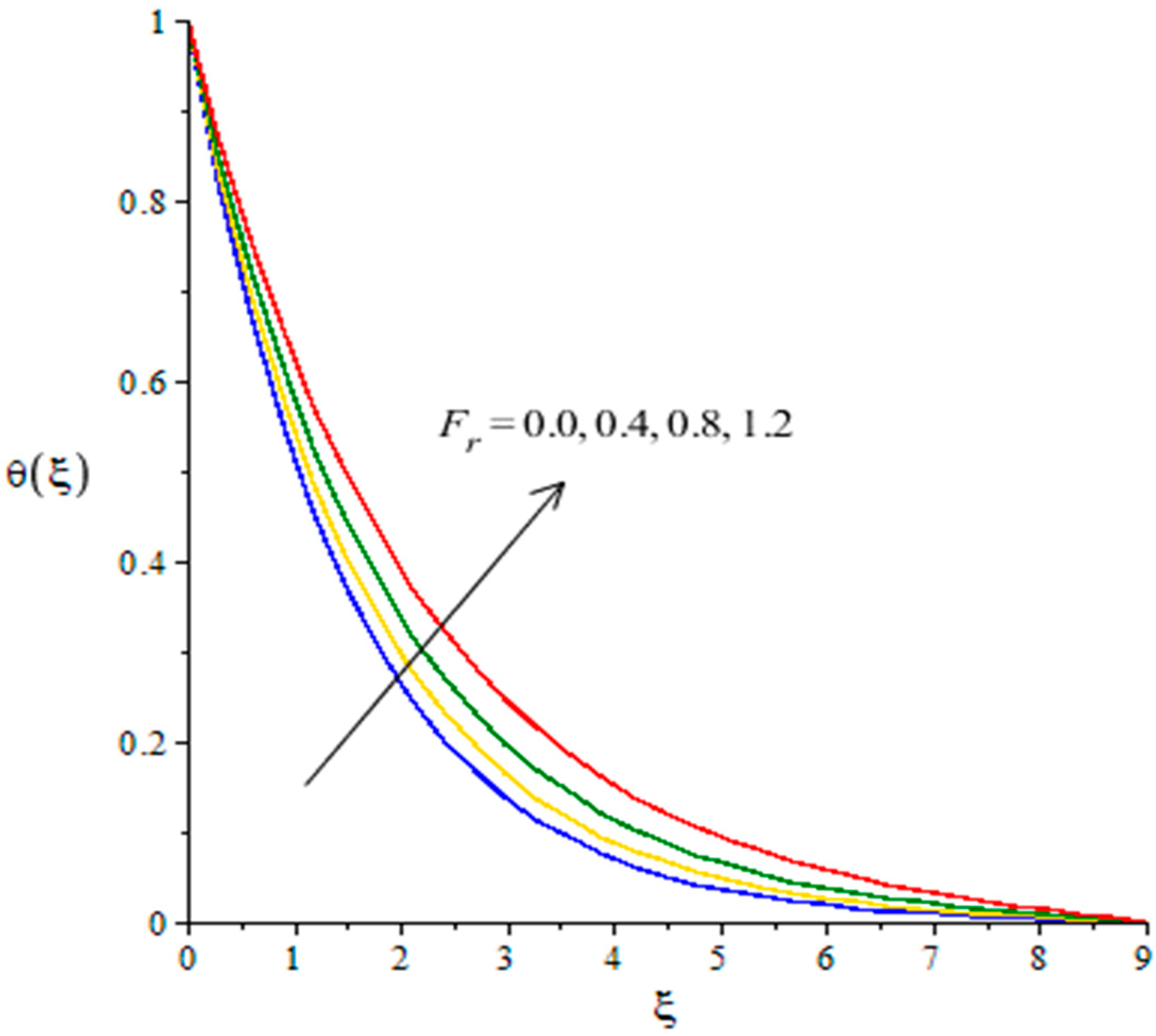
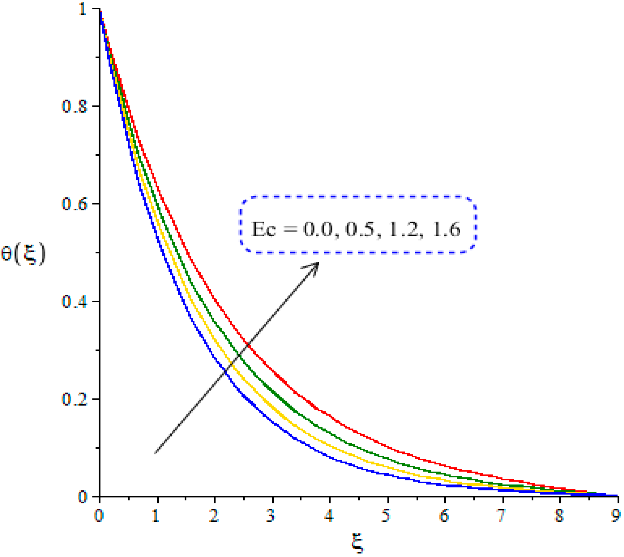
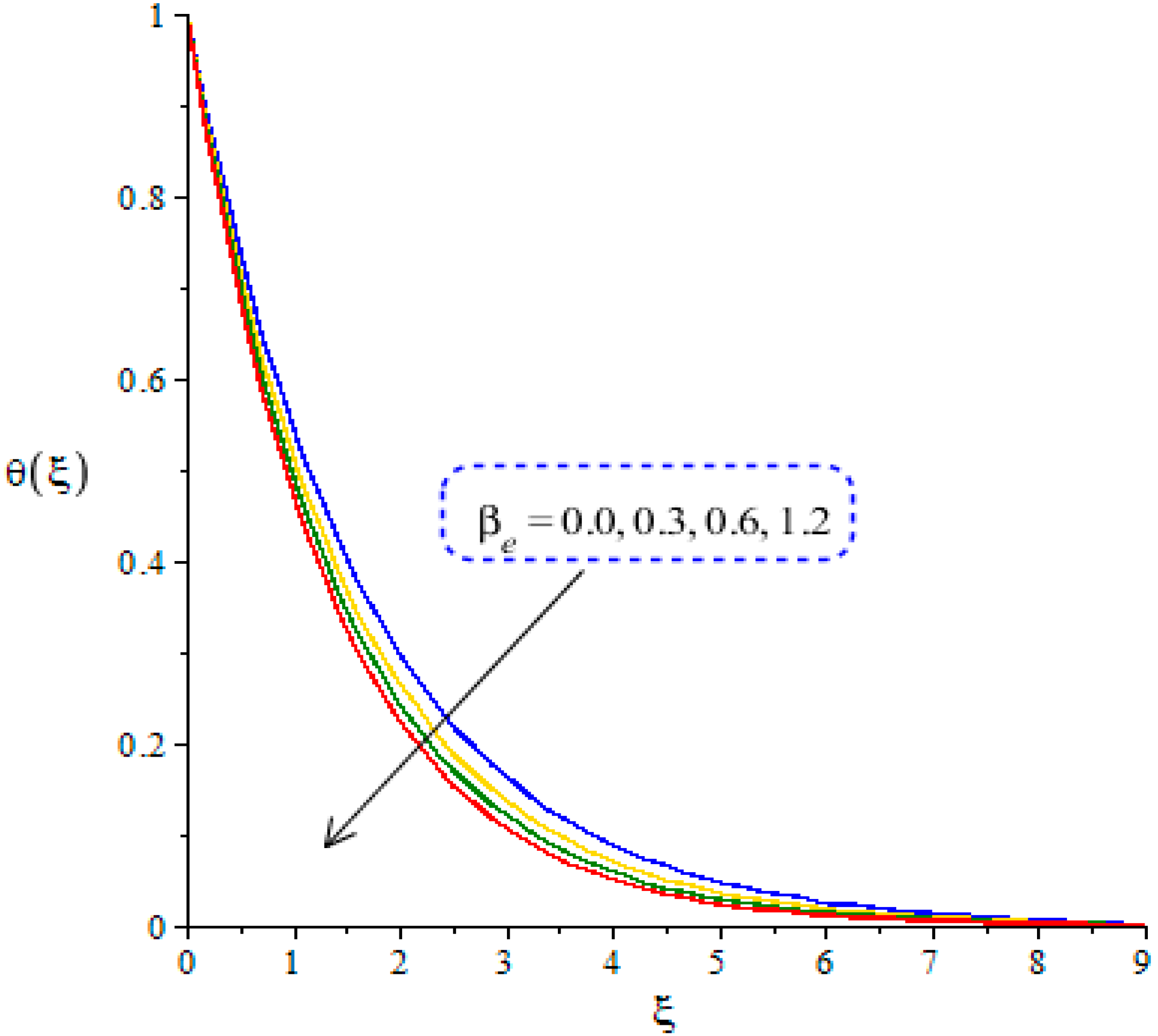
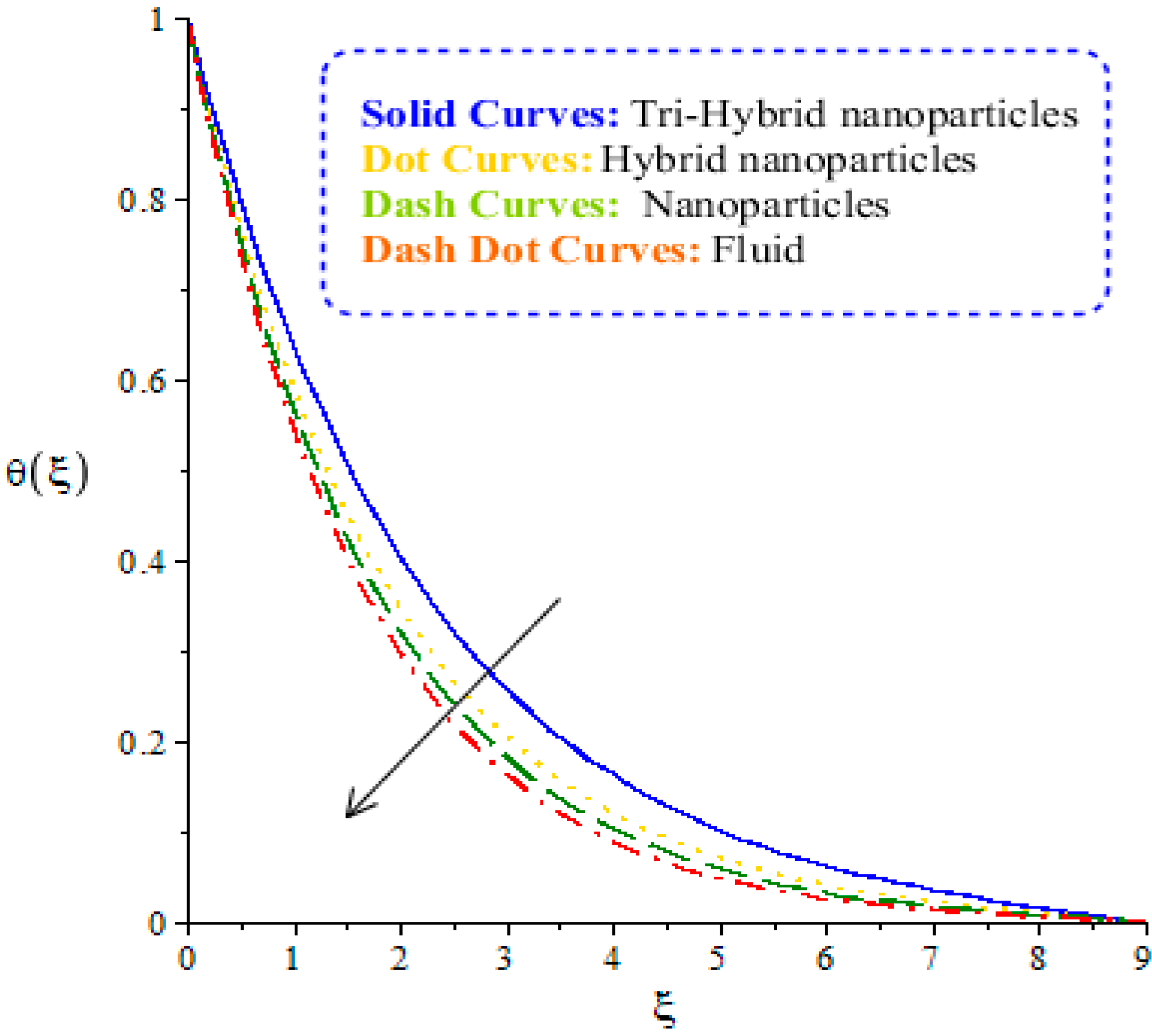
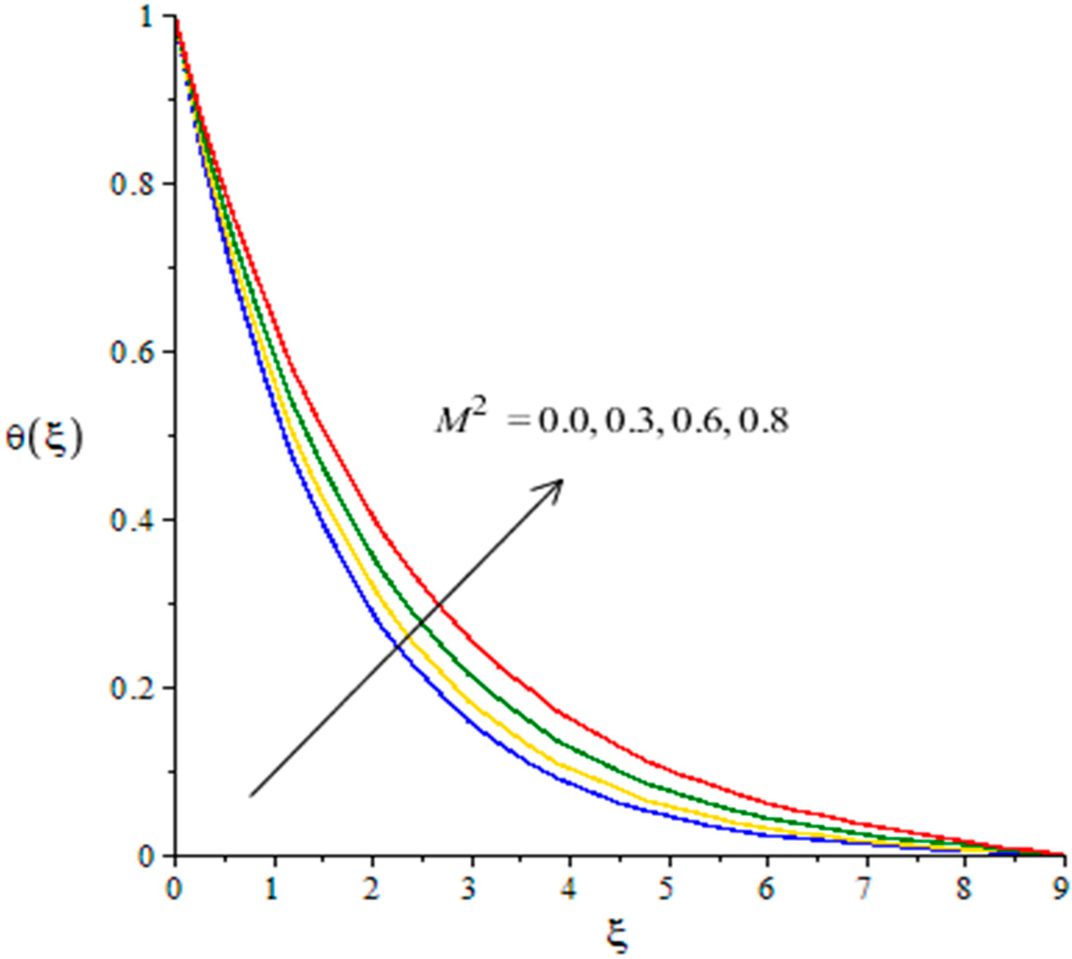
4.2. Outcomes of Temperature Profile versus Parameters

Heat production is measured, considering the impacts of the Eckert number, Hall number, ion-slip number, magnetic number and Forchheimer number, as shown in Figure 13, Figure 14, Figure 15, Figure 16, Figure 17 and Figure 18. Figure 16 visualizes the impact of nanoparticles, fluid, hybrid nanoparticles and tri-hybrid nanoparticles on the temperature profile. Figure 13 manufactures the production of heat energy in the motion of particles versus the variation in the Eckert number. The existence of $Ec$ is formulated due to the influence of viscous dissipation because $Ec$ occurred in a coefficient form of the viscous dissipation term. Viscous dissipation is known as work conducted, while the rate of work conducted is increased via large values $Ec.$ Further, work conducted is utilized in the motion of fluid particles, and the internal energy of fluid particles is boosted with the help of work conducted. Meanwhile, the temperature of particles increased. $Ec$ is used to determine the kinetic energy during flows in nanoparticles and hybrid nanoparticles. Further, this parameter is used to conduct enthalpy differences across boundary layers related to thermal energy, while $Ec$ is significantly used to measure heat dissipation in the motion of fluid particles. Figure 14 and Figure 15 are plotted to show heat production against the impacts of the ion-slip and Hall numbers, inserting tri-hybrid nanoparticles. The occurrence of the ion-slip and Hall numbers are modeled due to the existence of a Joule heating term. Heat energy decays when the ion-slip and Hall numbers are boosted. Mathematically, the ion-slip and Hall numbers are modeled in the Joule heating term (appearing as the denominator). Therefore, an inverse relationship is captured among heat energy, and ion-slip and Hall numbers. Consequently, the production of heat energy declines when the ion-slip and Hall numbers are boosted. Thickness regarding thermal layers also decreases via higher values of ion-slip and Hall numbers. Physically, this declining trend in producing heat energy occurs due to the phenomenon of Ohmic dissipation. The thickness associated within thermal boundary layers is controlled using partially ionized fluid under the action of a magnetic field. The thermal boundary layer (TBL) decreases against the higher impact of ion-slip and Hall numbers. Figure 16 reveals the vital role of tri-hybrid nanoparticles in the heat energy of particles. The comparative consequences among fluid, hybrid nanoparticles, nanoparticles and tri-hybrid nanoparticles are analyzed by the thermal performance of heat energy. The heat production for the case of tri-hybrid nanoparticles is investigated more efficiently than the heat production for fluid, nanoparticles and hybrid nanoparticles. Finally, it is concluded that the appearance of tri-hybrid nanoparticles plays an important role for the maximum production of heat energy. In view of thermal layers, thermal layers for a case of fluid are less than thermal layers for a case of nanoparticles, hybrid nanoparticles and tri-hybrid nanoparticles. Argumentation in the thermal energy of tri-hybrid nanoparticles is measured against variations in the magnetic number, as shown in Figure 17. The appearance of $M^2$ happens due to the effect of Joule heating in the energy equation. $M^2$ brings argumentation into the thermal energy when Joule heating is significant. The impact of $F_r$ is visualized on the temperature profile, while these effects are carried out by Figure 18. It is estimated that argumentation is investigated in heat energy against the distribution in $F_r$. The direct relation is formulated among $F_r$ and thermal energy.

4.3. Variation of Temperature Gradient and Surface Forces versus Parameters

The prediction of a temperature gradient and drag forces is visualized against variations in $F_r,{\beta }_i$ and ${\beta }_e$. This prediction is highlighted in Table 4. Numerical results are compared with the studies reported in [33], which are shown with the help of

Table 3. Comparative results of skin friction coefficients when $m=0.0,We=0.0,M^2=0.0,{\beta }_e=0.0,{\beta }_i=0.0,ϵ=0.0,F_r=0.0,Pr=2.04,Ec=2.0,{\phi }_2=0.0,{\phi }_1=0.0,{\phi }_3=0.0$.

$\mathbf{\Omega }.$	Hussain et al. [33]		Present Results
	$-{\left(\mathit{R}\mathit{e}\right)}^{1/2}{\mathit{C}}_{\mathit{F}}$	$-{\left(\mathit{R}\mathit{e}\right)}^{1/2}{\mathit{C}}_{\mathit{G}}$	$-{\left(\mathit{R}\mathit{e}\right)}^{1/2}{\mathit{C}}_{\mathit{F}}$	$-{\left(\mathit{R}\mathit{e}\right)}^{1/2}{\mathit{C}}_{\mathit{G}}$
0.0	1.00426	0.0	1.000431019	0.0
0.5	1.17189	0.5488	1.171210113	1.172901620
1.0	1.3582	0.8589	1.358181503	1.357812653
2.0	1.68033	1.3027	1.681031011	1.681061039

. Drag forces declined versus the variation in ion-slip and Hall numbers, while drag forces inclined when the impact of $F_r$ was enhanced in the existence of tri-hybrid nanoparticles. Moreover, the temperature gradient enhanced using variation in ${\beta }_i$ and ${\beta }_e.$ However, the production of the temperature gradient is boosted via variation in $F_r$, which is monitored in

Table 4. Numerical values of coefficients related to skin friction coefficients and the Nusselt number against variations in ${\beta }_e,{\beta }_i$ and $F_r$ by inserting tri-hybrid nanoparticles when $m=0.1,We=2,\mathsf{\Omega }=2.0,M^2=0.5,ϵ=0.03,Pr=204,Ec=0.7,{\phi }_2=0.0075,{\phi }_1=0.002,{\phi }_3=0.005$.

		$-{\left(\mathit{R}\mathit{e}\right)}^{1/2}{\mathit{C}}_{\mathit{F}}$	$-{\left(\mathit{R}\mathit{e}\right)}^{1/2}{\mathit{C}}_{\mathit{G}}$	${\left(\mathit{R}\mathit{e}\right)}^{-1/2}\mathit{N}\mathit{u}$
	0.1	0.295179854	0.1142831221	0.30548038
${\beta }_e$	0.3	0.194084007	0.2967735778	0.60158358
	0.6	0.026758931	0.3730140256	0.89567749
	0.1	0.445563794	0.2710562039	0.54590968
${\beta }_i$	0.4	0.436878968	0.2363434625	0.56018140
	0.8	0.414948438	0.2214122528	0.59544356
	0.0	0.524948431	0.2714123242	0.49545303
$F_r$	0.3	0.534948431	0.2814123838	0.43545891
	0.6	0.554948434	0.2914124206	0.41546269

.

5. Remarks and Key Judgments

In the present analysis, tri-hybrid nano-structures are inserted into the motion and heat energy of fluid particles. The generalized Ohm’s theory is considered under the action of a constant magnetic field. Viscous dissipation and Joule heating terms are modeled. The numerical scheme, known as the finite element approach, is implemented to show the numerical and graphical consequences. The main points of this analysis are listed below:

❖

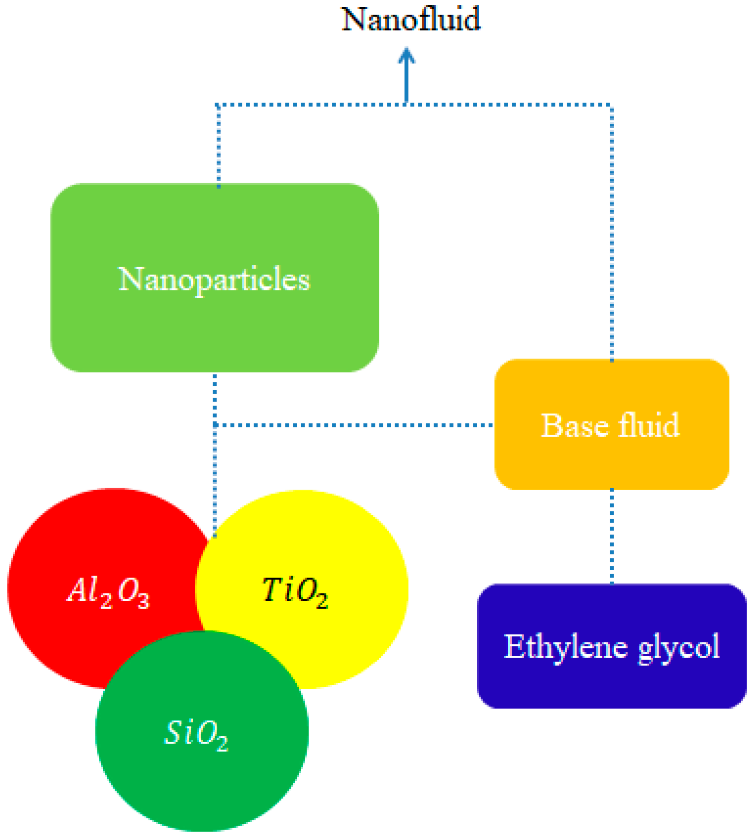
Ternary hybrid nanoparticles play a vital role in enhancing the performance of heat energy. Moreover, heat energy is produced by hybrid nanoparticles, nanoparticles and nanofluid;

❖

Argumentation in the motion of the fluid is predicted using the higher values of ion-slip and Hall numbers, while the opposite treatment is found in the motion of fluid particles via variation in the Weissenberg and Forchheimer numbers;

❖

The maximum production of thermal energy occurs when the Eckert number is increased, and declination in heat energy occurs via higher values of ion-slip and Hall numbers;

❖

The maximum production of a temperature gradient can be achieved for the case of ternary hybrid nanoparticles, rather than the production of a temperature gradient for the cases of nanoparticles and hybrid nanoparticles;

❖

Ternary hybrid nanoparticles boost the surface force, as compared to nanoparticles and hybrid nanoparticles;

❖

Hall and ion-slip currents are significantly useful to enhance the temperature gradient, but the surface force is boosted when Hall and ion-slip numbers are enhanced.

References

1. Khan, M.; Rasheed, A.; Salahuddin, T.; Ali, S. Chemically reactive flow of hyperbolic tangent fluid flow having thermal radiation and double stratification embedded in porous medium. Ain Shams Eng. J. 2021, 12, 3209–3216. [Google Scholar] [CrossRef]
2. Rehman, K.U.; Alshomrani, A.S.; Malik, M.Y.; Zehra, I.; Naseer, M. Thermo-physical aspects in tangent hyperbolic fluid flow regime: A short communication. Case Stud. Therm. Eng. 2018, 12, 203–212. [Google Scholar] [CrossRef]
3. Khan, M.; Rasheed, A.; Salahuddin, T. Radiation and chemical reactive impact on tangent hyperbolic fluid flow having double stratification. AIP Adv. 2020, 10, 075211. [Google Scholar] [CrossRef]
4. Gharami, P.P.; Reza-E-Rabbi, S.; Arifuzzaman, S.M.; Khan, M.S.; Sarkar, T.; Ahmmed, S.F. MHD effect on unsteady flow of tangent hyperbolic nano-fluid past a moving cylinder with chemical reaction. SN Appl. Sci. 2020, 2, 1256. [Google Scholar] [CrossRef]
5. Hayat, T.; Shafique, M.; Tanveer, A.; Alsaedi, A. Magnetohydrodynamic effects on peristaltic flow of hyperbolic tangent nanofluid with slip conditions and Joule heating in an inclined channel. Int. J. Heat Mass Transf. 2016, 102, 54–63. [Google Scholar] [CrossRef]
6. Nawaz, M.; Madkhali, H.A.; Haneef, M.; Alharbi, S.O.; Alaoui, M.K. Numerical study on thermal enhancement in hyperbolic tangent fluid with dust and hybrid nanoparticles. Int. Commun. Heat Mass Transf. 2021, 127, 105535. [Google Scholar] [CrossRef]
7. Wang, X.Q.; Mujumdar, A.S. A review on nanofluids-part I: Theoretical and numerical investigations. Braz. J. Chem. Eng. 2008, 25, 613–630. [Google Scholar] [CrossRef] [Green Version]
8. Tlau, L. Fundamental flow problems considering non-Newtonian hyperbolic tangent fluid with Navier slip: Homotopy analysis method. Appl. Comput. Mech. 2020, 14. [Google Scholar] [CrossRef]
9. Kebede, T.; Haile, E.; Awgichew, G.; Walelign, T. Heat and mass transfer analysis in unsteady flow of tangent hyperbolic nanofluid over a moving wedge with buoyancy and dissipation effects. Heliyon 2020, 6, e03776. [Google Scholar] [CrossRef]
10. Saidulu, N.; Gangaiah, T.; Lakshmi, A.V. MHD flow of tangent hyperbolic nanofluid over an inclined sheet with effects of thermal radiation and heat source/sink. Appl. Appl. Math. Int. J. 2019, 14, 5. [Google Scholar]
11. Mahdy, A.; Hoshoudy, G.A. Two-phase mixed convection nanofluid flow of a dusty tangent hyperbolic past a nonlinearly stretching sheet. J. Egypt. Math. Soc. 2019, 27, 44. [Google Scholar] [CrossRef] [Green Version]
12. Shafiq, A.; Hammouch, Z.; Sindhu, T.N. Bioconvective MHD flow of tangent hyperbolic nanofluid with newtonian heating. Int. J. Mech. Sci. 2017, 133, 759–766. [Google Scholar] [CrossRef]
13. Hayat, T.; Qayyum, S.; Alsaedi, A.; Shehzad, S.A. Nonlinear thermal radiation aspects in stagnation point flow of tangent hyperbolic nanofluid with double diffusive convection. J. Mol. Liq. 2016, 223, 969–978. [Google Scholar] [CrossRef]
14. Shafiq, A.; Lone, S.A.; Sindhu, T.N.; Al-Mdallal, Q.M.; Rasool, G. Statistical modeling for bioconvective tangent hyperbolic nanofluid towards stretching surface with zero mass flux condition. Sci. Rep. 2021, 11, 13869. [Google Scholar] [CrossRef]
15. Swain, K.; Mebarek-Oudina, F.; Abo-Dahab, S.M. Influence of MWCNT/ Fe 3 O 4 hybrid nanoparticles on an exponentially porous shrinking sheet with chemical reaction and slip boundary conditions. J. Therm. Anal. Calorim. 2021, 143, 915–927. [Google Scholar]
16. Shafiq, A.; Mebarek-Oudina, F.; Sindhu, T.N.; Abidi, A. A study of dual stratification on stagnation point Walters’ B nanofluid flow via radiative Riga plate: A statistical approach. Eur. Phys. J. Plus 2021, 136, 407. [Google Scholar] [CrossRef]
17. Mebarek-Oudina, F.; Fares, R.; Aissa, A.; Lewis, R.W.; Abu-Hamdeh, N.H. Entropy and convection effect on magnetized hybrid nano-liquid flow inside a trapezoidal cavity with zigzagged wall. Int. Commun. Heat Mass Transf. 2021, 125, 105279. [Google Scholar] [CrossRef]
18. Marzougui, S.; Mebarek-Oudina, F.; Magherbi, M.; Mchirgui, A. Entropy generation and heat transport of Cu–water nanoliquid in porous lid-driven cavity through magnetic field. Int. J. Numer. Methods Heat Fluid Flow 2021. [Google Scholar] [CrossRef]
19. Pushpa, B.V.; Sankar, M.; Mebarek-Oudina, F. Buoyant Convective Flow and Heat Dissipation of Cu– H 2 O Nanoliquids in an Annulus Through a Thin Baffle. J. Nanofluids 2021, 10, 292–304. [Google Scholar] [CrossRef]
20. Upreti, H.; Pandey, A.K.; Kumar, M.; Makinde, O.D. Ohmic heating and non-uniform heat source/sink roles on 3D Darcy–Forchheimer flow of CNTs nanofluids over a stretching surface. Arab. J. Sci. Eng. 2020, 45, 7705–7717. [Google Scholar] [CrossRef]
21. Upreti, H.; Pandey, A.K.; Kumar, M. Thermophoresis and suction/injection roles on free convective MHD flow of Ag–kerosene oil nanofluid. J. Comput. Des. Eng. 2020, 7, 386–396. [Google Scholar] [CrossRef]
22. Upreti, H.; Pandey, A.K.; Kumar, M. Assessment of entropy generation and heat transfer in three-dimensional hybrid nanofluids flow due to convective surface and base fluids. J. Porous Media 2021, 24, 35–50. [Google Scholar] [CrossRef]
23. Abdelsalam, S.I.; Sohail, M. Numerical approach of variable thermophysical features of dissipated viscous nanofluid comprising gyrotactic micro-organisms. Pramana: J. Phys. 2020, 94, 67. [Google Scholar] [CrossRef]
24. Sohail, M.; Shah, Z.; Tassaddiq, A.; Kumam, P.; Roy, P. Entropy generation in MHD Casson fluid flow with variable heat conductance and thermal conductivity over non-linear bi-directional stretching surface. Sci. Rep. 2020, 10, 12530. [Google Scholar] [CrossRef]
25. Thumma, T.; Wakif, A.; Animasaun, I.L. Generalized differential quadrature analysis of unsteady three-dimensional MHD radiating dissipative Casson fluid conveying tiny particles. Heat Transf. 2020, 49, 2595–2626. [Google Scholar] [CrossRef]
26. Chu, Y.M.; Nazir, U.; Sohail, M.; Selim, M.M.; Lee, J.R. Enhancement in Thermal Energy and Solute Particles Using Hybrid Nanoparticles by Engaging Activation Energy and Chemical Reaction over a Parabolic Surface via Finite Element Approach. Fractal Fract. 2021, 5, 119. [Google Scholar] [CrossRef]
27. Nazir, U.; Sohail, M.; Ali, U.; Sherif, E.S.M.; Park, C.; Lee, J.R.; Selim, M.M.; Thounthong, P. Applications of Cattaneo–Christov fluxes on modelling the boundary value problem of Prandtl fluid comprising variable properties. Sci. Rep. 2021, 11, 17837. [Google Scholar] [CrossRef] [PubMed]
28. Wakif, A.; Boulahia, Z.; Ali, F.; Eid, M.R.; Sehaqui, R. Numerical analysis of the unsteady natural convection MHD Couette nanofluid flow in the presence of thermal radiation using single and two-phase nanofluid models for Cu–water nanofluids. Int. J. Appl. Comput. Math. 2018, 4, 81. [Google Scholar] [CrossRef]
29. Nazir, U.; Sohail, M.; Alrabaiah, H.; Selim, M.M.; Thounthong, P.; Park, C. Inclusion of hybrid nanoparticles in hyperbolic tangent material to explore thermal transportation via finite element approach engaging Cattaneo-Christov heat flux. PLoS ONE 2021, 16, e0256302. [Google Scholar] [CrossRef] [PubMed]
30. Hayat, T.; Aziz, A.; Muhammad, T.; Alsaedi, A. Darcy-Forchheimer flow of nanofluid in a rotating frame. Int. J. Numer. Methods Heat Fluid Flow 2018. [Google Scholar] [CrossRef]
31. Hayat, T.; Aziz, A.; Muhammad, T.; Alsaedi, A. Three-dimensional flow of Prandtl fluid with Cattaneo-Christov double diffusion. Results Phys. 2018, 9, 290–296. [Google Scholar] [CrossRef]
32. Manjunatha, S.; Puneeth, V.; Gireesha, B.J.; Chamkha, A. Theoretical Study of Convective Heat Transfer in Ternary Nanofluid Flowing past a Stretching Sheet. J. Appl. Comput. Mech. 2021. [Google Scholar] [CrossRef]
33. Hussain, A.; Elkotb, M.A.; Arshad, M.; Rehman, A.; Sooppy Nisar, K.; Hassan, A.; Saleel, C.A. Computational investigation of the combined impact of nonlinear radiation and magnetic field on three-dimensional rotational nanofluid flow across a stretchy surface. Processes 2021, 9, 1453. [Google Scholar] [CrossRef]
Figure 1. Prepared scheme of hybrid nanostructures.
Energies 14 06911 g001
Figure 2. Coordinate system and physical illustration.
Energies 14 06911 g002
Figure 3. Variation role of G ( ξ ) versus W e when m = 0.5 ,   Ω = 3.0 ,   M 2 = 0.1 ,   β e = 0.3 ,   β i = 0.1 ,   ϵ = 0.04 ,   F r = 2.0 ,   P r = 204 ,   E c = 0.3 ,   φ 2 = 0.0075 ,   φ 1 = 0.002 ,   φ 3 = 0.005 .
Energies 14 06911 g003
Figure 4. Variation role of F ( ξ ) versus W e when m = 0.3 ,   Ω = 3.0 ,   M 2 = 0.3 ,   β e = 0.5 ,   β i = 0.7 ,   ϵ = 0.01 ,   F r = 3.5 ,   P r = 204 ,   E c = 3.0 ,   φ 2 = 0.0075 ,   φ 1 = 0.002 ,   φ 3 = 0.005 .
Energies 14 06911 g004
Figure 5. Variation role of G ( ξ ) versus F r when m = 0.4 ,   W e = 5 ,   Ω = 2.0 ,   M 2 = 0.1 ,   β e = 0.5 ,   β i = 0.3 ,   ϵ = 0.01 ,   P r = 204 ,   E c = 0.4 ,   φ 2 = 0.0075 ,   φ 1 = 0.002 ,   φ 3 = 0.005 .
Energies 14 06911 g005
Figure 6. Variation role of F ( ξ ) versus F r when m = 0.3 ,   W e = 3 ,   Ω = 2.0 ,   M 2 = 0.33 ,   β e = 0.2 ,   β i = 0.01 ,   ϵ = 0.01 ,   P r = 204 ,   E c = 0.34 ,   φ 2 = 0.0075 ,   φ 1 = 0.002 ,   φ 3 = 0.005 .
Energies 14 06911 g006
Figure 7. Variation role of G ( ξ ) versus F r when m = 0.7 ,   W e = 4.0 ,   Ω = 2.3 ,   M 2 = 0.3 ,   β i = 0.2 ,   ϵ = 0.1 ,   F r = 2.7 ,   P r = 204 ,   E c = 0.14 ,   φ 2 = 0.0075 ,   φ 1 = 0.002 ,   φ 3 = 0.005 .
Energies 14 06911 g007
Figure 8. Variation role of F ( ξ ) versus F r when m = 0.01 ,   W e = 5 ,   Ω = 2.0 ,   M 2 = 0.5 ,   β i = 0.3 ,   ϵ = 0.1 ,   F r = 2.7 ,   P r = 204 ,   E c = 0.14 ,   φ 2 = 0.0075 ,   φ 1 = 0.002 ,   φ 3 = 0.005 .
Energies 14 06911 g008
Figure 9. Variation role of G ( ξ ) versus F r when m = 0.3 ,   W e = 5 ,   Ω = 3.0 ,   M 2 = 0.01 ,   β e = 0.3 ,   ϵ = 0.5 ,   F r = 2.0 ,   P r = 204 ,   E c = 0.7 ,   φ 2 = 0.0075 ,   φ 1 = 0.002 ,   φ 3 = 0.005 .
Energies 14 06911 g009
Figure 10. Variation role of F ( ξ ) versus F r when m = 0.1 ,   W e = 2.5 ,   Ω = 2.0 ,   M 2 = 0.3 ,   β e = 0.5 ,   ϵ = 0.1 ,   F r = 2.5 ,   P r = 204 ,   E c = 0.3 ,   φ 2 = 0.0075 ,   φ 1 = 0.002 ,   φ 3 = 0.005 .
Energies 14 06911 g010
Figure 11. Variation role of F ( ξ ) versus Ω when m = 0.01 ,   W e = 7 ,   M 2 = 0.1 ,   β e = 0.7 ,   β i = 0.31 ,   ϵ = 0.04 ,   F r = 3.0 ,   P r = 204 ,   E c = 0.34 ,   φ 2 = 0.0075 ,   φ 1 = 0.002 ,   φ 3 = 0.005 .
Energies 14 06911 g011
Figure 12. Variation role of G ( ξ ) versus Ω when m = 0.21 ,   W e = 7 ,   M 2 = 0.4 ,   β e = 0.52 ,   β i = 0.3 ,   ϵ = 0.01 ,   F r = 2.0 ,   P r = 204 ,   E c = 0.34 ,   φ 2 = 0.0075 ,   φ 1 = 0.002 ,   φ 3 = 0.0071 .
Energies 14 06911 g012
Figure 13. Variation role of θ ( ξ ) versus E c when m = 0.3 ,   W e = 3 ,   Ω = 2.0 ,   M 2 = 0.3 ,   β e = 0.5 ,   β i = 0.7 ,   ϵ = 0.01 ,   F r = 2.5 ,   P r = 204 ,   φ 2 = 0.0075 ,   φ 1 = 0.002 ,   φ 3 = 0.005 .
Energies 14 06911 g013
Figure 14. Variation role of θ ( ξ ) versus β e when m = 0.43 ,   W e = 5.0 ,   Ω = 3.0 ,   M 2 = 0.34 ,   β i = 0.3 ,   ϵ = 0.3 ,   F r = 2.0 ,   P r = 204 ,   E c = 0.3 ,   φ 2 = 0.0075 ,   φ 1 = 0.002 ,   φ 3 = 0.005 .
Energies 14 06911 g014
Figure 15. Variation role of θ ( ξ ) versus β i when m = 0.1 ,   W e = 3 ,   Ω = 2.0 ,   M 2 = 0.3 ,   β e = 0.5 ,   ϵ = 0.34 ,   F r = 2.0 ,   P r = 204 ,   E c = 0.3 ,   φ 2 = 0.0075 ,   φ 1 = 0.002 ,   φ 3 = 0.005 .
Energies 14 06911 g015
Figure 16. Comparative investigation among fluid, nanoparticles, hybrid nanoparticles and tri-hybrid nanoparticles on temperature profile when m = 0.1 ,   W e = 5 ,   Ω = 2.0 ,   M 2 = 0.3 ,   β e = 0.5 ,   β i = 0.7 ,   ϵ = 0.01 ,   F r = 2.5 ,   P r = 204 ,   E c = 0.54 ,   φ 2 = 0.0075 ,   φ 1 = 0.002 ,   φ 3 = 0.005 .
Energies 14 06911 g016
Figure 17. Variation role of θ ( ξ ) versus M 2 when m = 0.01 ,   W e = 3 ,   Ω = 3.0 ,   β e = 0.5 ,   β i = 0.7 ,   ϵ = 0.01 ,   F r = 2.5 ,   P r = 204 ,   E c = 0.34 ,   φ 2 = 0.0075 ,   φ 1 = 0.002 ,   φ 3 = 0.005 .
Energies 14 06911 g017
Figure 18. Variation role of θ ( ξ ) versus F r when m = 0.12 ,   W e = 5 ,   Ω = 2.0 ,   M 2 = 0.3 ,   β e = 0.5 ,   β i = 0.4 ,   ϵ = 0.1 ,   P r = 204 ,   E c = 0.34 = 5.0 ,   φ 2 = 0.0075 ,   φ 1 = 0.002 ,   φ 3 = 0.005 .
Energies 14 06911 g018