An Immersed Boundary–Lattice Boltzmann Approach to Study Deformation and Fluid–Structure Interaction of Hollow Sealing Strip

Abstract

A combined immersed boundary–lattice Boltzmann approach is used to simulate the dynamics of the fluid–structure interaction of a hollow sealing strip under the action of pressure difference. Firstly, the multiple relaxation times LBM model, hyper-elastic material model and immersed boundary method were deduced. According to the strain characteristics of hyper-elastic materials and the specific situation of friction between the elastic boundary and solid boundary, the internal force and the external force on the immersed boundary were discussed and deduced, respectively. Then, a 2D calculation model of the actual hollow sealing strip system was established, during which technical problems such as the equivalent wall thickness of the sealing strip and the correction of the stiffness of the contact corner were solved. The reliability of the model was verified by comparing results of FEM simulation of quasi-static deformation. Following this, the simulation results of three typical cases of sealing strips were presented. The results show that when the sealing strip fails, there will be a strong coupling phenomenon between the flow field and the sealing strip, resulting in the oscillation of the flow field and the sealing strip at the same frequency.

1. Introduction

Due to its large deformable range and small pressing force, the hollow sealing strip is widely used in door sealing of automobiles and airplanes [1]. When a vehicle is moving at high speed, there will be a large pressure difference inside and outside the passenger compartment, which is more serious on aircraft. The pressure difference between the two sides not only produces an extrusion effect on the sealing strip, but also produces an external suction effect on the door due to the lower outer pressure, which greatly reduces the pre-compression shrinkage of the seal [2]. In that case, the sealing strip may fail, and the air in the gap will flow due to the pressure difference, resulting in strong aspiration noise [3]. In the process of seal failure, the change of the flow field around the seal is coupled with the elastic deformation of the seal, forming a fluid–structure interaction (FSI) [4,5], which makes the research of this kind of seal very difficult. In addition, the pressure inside the hollow sealing strip also has an important influence on the deformation, failure and fluid–structure interaction of the sealing strip, which is usually simplified as the treatment of internal steady pressure in traditional methods, which brings more errors to the analysis [6].

Ethylene propylene diene monomer (EPDM) is the most commonly used material type of the hollow sealing strip, which is a typical hyper-elastic material with obvious nonlinear mechanical properties. As early as 1940, Mooney proposed using a nonlinear model to express the mechanical properties of materials [7]. For the description of mechanical properties of rubber materials, the semi-empirical method is the most effective method in engineering applications based on the continuous medium model and experimental measurement. Among them, the third-order strain energy function model proposed by Ogden can well-express the hyper-elastic properties of rubber materials [8]. In addition, the model proposed by Rivlin on the basis of Mooney’s theory (Mooney–Rivlin model) is also widely used [9].

With the mechanical model of the material, it is convenient to simulate the sealing system by using the finite element method (FEM). The pre-compression deformation of the sealing strip [10] and the deformation and failure under the static fluid pressure difference [11,12] can be simulated accurately. The main defect of FEM to simulate the failure process of the sealing strip is that it only transforms the fluid action on a solid into a steady surface force, but does not simulate the flow and lead to a change of force after fluid movement. In order to simulate the seal strip and fluid coupling accurately, the fluid–structure interaction simulation must be combined with computational fluid dynamics (CFD). Traditional numerical methods for solving FSI problems use body-fitted and moving mesh approaches, such as the arbitrary Lagrangian Eulerian (ALE) [13] method and the transforming spatial domain/stabilized space–time (DSD/SST) method [14]. In these methods, the grid is distributed, and in order to avoid serious grid distortion, it is usually necessary to regenerate the grid every few time steps, so the calculation is very cumbersome and consumes a lot of computing resources. For these reasons, the FSI simulation technology combining the immersed boundary method (IBM) and the lattice Boltzmann method (LBM) has developed rapidly in recent years [15,16]. It is based on non-conformal Cartesian meshes, so they are more efficient in dealing with complex and moving geometry.

LBM is derived from the theory of gas dynamics, which is quite different from the traditional CFD method based on the discretization of the macro-continuum equation. The governing equations of LBM are in an explicit form, so numerical solutions and parallel computation are easier. The easy implementation of curve boundary conditions makes the mesh generation of LBM very simple. In addition, the flow field of LBM is always compressible, and when the incompressible problem needs to be solved, the incompressible N-S equation can be obtained under the approximate incompressible limit [17]. Therefore, LBM has great advantages in solving the problems of compressible flow [18,19], aerodynamic noise [20,21], particle suspension fluid [22] and multi-phase flow [23,24], which consume a lot of computational resources in traditional CFD.

IBM was first proposed by Peskin [25] in 1977. In this method, the solid structure is regarded as a boundary immersed in fluid, which can be represented by the singular force in the Navier–Stokes (N-S) equation to simulate the no-slip condition on the structure [26]. IBM uses a mixture of Euler variables defined on a fixed Cartesian mesh and Lagrangian variables defined on a curved mesh, on top of the fixed Cartesian mesh representing the immersed boundary. Two kinds of variables are connected by the smooth approximation of the Dirac delta function. The Lagrangian force on the immersed flexible boundaries can be derived from the principle of virtual work [27].

According to their principles, the combination of IBM and LBM has natural advantages in numerical format, solution method and grid processing, so the IB-LBM method has been widely utilized [28]. This method is particularly effective for the fluid–structure interaction problem of the elastic body with a negligible mass in fluid, so it was initially applied to the biological fluid problem [29,30,31] very well. In recent years, great progress has been made in strong fluid–structure interaction- [32,33] and particle flow [34,35,36].

The present study aims to use IB-LBM to investigate the fluid–structure interaction simulation problem of the sealing strip. One of the characteristics of this study is that the elastic boundary, which is represented by the immersed boundary, is a rubber material, and its strain characteristics are nonlinear. It is necessary to establish a relationship between the material empirical model and the immersed boundary. Another feature of this study is that the immersed boundary is not always completely immersed in the fluid, it will also squeeze, friction and slip with the rigid wall, making the dynamic characteristics of the immersed boundary more complex.

After solving the above two problems, taking the actual hollow sealing strip as the research object, a two-dimensional calculation model was established. In the process of simulating the real sealing strip using the non-thickness immersed boundary, the technical problems such as the equivalent wall thickness of the sealing strip and the correction of the stiffness of the contact corner were also solved.

The effectiveness of the IB model was verified by the FEM simulation of the same sealing strip. After completing the modeling, the fluid–structure interaction simulation was carried out for three typical conditions, which are non-failure, absolute failure and dynamic failure of the sealing strip, and the specific relationship between the deformation of the sealing strip and the fluid movement was analyzed.

2. Immersed Boundary–Lattice Boltzmann Method

2.1. LBM Governing Equation

The LBM collision operator used in this paper is the multiple relaxation times (MRT) model [37]. Its relaxation parameters are expressed by different physical quantities, such as fluid density, kinetic energy, momentum, energy flux and viscous stress tensor. These physical quantities can be relaxed to their respective equilibrium states with different relaxation times, which increases the flexibility of the algorithm. Therefore, compared to the single relaxation time (SRT) [38], the MRT model can reduce the fluctuation of the pressure field and the velocity field caused by false oscillation modes on the grid scale, and then improve the stability and calculation accuracy of the algorithm. The governing equation of MRT-LBM is:

$$f_i\left(\mathit{x}+{\mathit{c}}_i\Delta t,t+\Delta t\right)-f_i\left(\mathit{x},t\right)=-{\mathit{M}}^{-1}\mathit{S}\mathit{M}[f_i\left(\mathit{x},t\right)-f_i^{eq}\left(\mathit{x},t\right)]+{\mathit{M}}^{-1}\left(\mathit{I}-\frac{1}{2}\mathit{S}\right)\mathit{M}{\mathit{F}}_i\Delta$$

(1)

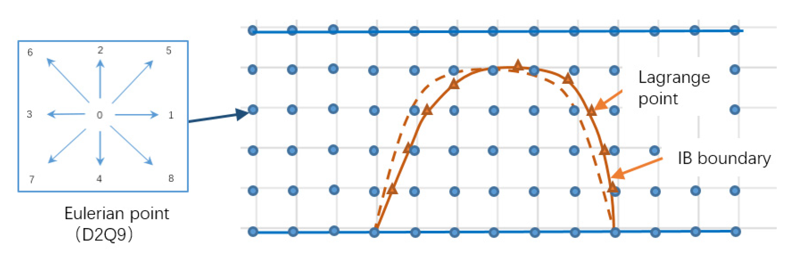
Here, the subscript $i$ represents the grid direction, as “0 ~ 9” shown on the left side of Figure 1, $\mathit{x}$ is the spatial coordinate of the flow field, $t$ is the time, $\Delta t$ is the time step, $f_i$ is the density distribution function in discrete form, $f_i^{eq}$ is the corresponding equilibrium distribution function and ${\mathit{F}}_i$ is the force term applied to the distribution function. $\mathit{I}$ is the unit diagonal matrix, and $\mathit{M}$ and $\mathit{S}$ are the mapping matrix and diagonal collision relaxation matrix, respectively, and their expressions are shown in Equations (2) and (3), where ${\upsilon }_l$ is the lattice kinematic viscosity.

$$\mathit{M}=[\begin{array}{ccccccccc}1& 1& 1& 1& 1& 1& 1& 1& 1\\ -4& -1& -1& -1& -1& 2& 2& 2& 2\\ 4& -2& -2& -2& -2& 1& 1& 1& 1\\ 0& 1& 0& -1& 0& 1& -1& -1& 1\\ 0& -2& 0& 2& 0& 1& -1& -1& 1\\ 0& 0& 1& 0& -1& 1& 1& -1& -1\\ 0& 0& -2& 0& 2& 1& 1& -1& -1\\ 0& 1& -1& 1& -1& 0& 0& 0& 0\\ 0& 0& 0& 0& 0& 1& -1& 1& -1\end{array}]$$

(2)

$$\mathit{S}=diag\left[01.11.0501.0501.05\frac{2}{6{\upsilon }_l-1}\frac{2}{6{\upsilon }_l-1}\right]$$

(3)

In addition, ${\mathit{c}}_i$ is the discrete velocity, which is defined in Formula (4) of the D2Q9 lattice model used in this paper, where $\Delta x$ is the lattice spacing:

$${\mathit{c}}_i=\{\begin{array}{c}\left(0,0\right), i=0\\ \left(\cos \left[\frac{\left(i-1\right)\pi }{2}\right],\sin \left[\frac{\left(i-1\right)\pi }{2}\right]\right)\frac{\Delta x}{\Delta t}, i=1~4\\ \sqrt{2}\left(\cos \left[\frac{\left(2i-1\right)\pi }{4}\right],\sin \left[\frac{\left(2i-1\right)\pi }{4}\right]\right)\frac{\Delta x}{\Delta t}, i=5~8\end{array}$$

(4)

In this model, $f_i^{eq}$ and $F_i$ are:

$$f_i^{eq}={\omega }_i\rho \left[1+\frac{{\mathit{c}}_i\mathit{u}}{c_s^2}+\frac{{\left({\mathit{c}}_i\mathit{u}\right)}^2}{2c_s^4}+\frac{{\mathit{u}}^2}{2{\mathit{c}}_s^2}\right]$$

(5)

$$F_i={\omega }_i\left(\frac{{\mathit{c}}_i-\mathit{u}}{c_s^2}+\frac{{\mathit{c}}_i·\mathit{u}}{c_s^4}{\mathit{c}}_i\right)·\mathit{F}$$

(6)

Here,$c_s=1/\sqrt{3}$ is the sound velocity under the lattice Boltzmann method, $\mathit{F}$ represents the physical force acting on the fluid, including viscoelastic force and introduction force at the immersed boundary, and ${\omega }_i$ is the weighting factor. In the D2Q9 model, ${\omega }_0=4/9$, ${\omega }_i=1/9$ when $i=1~4$ and ${\omega }_i=1/36$ when $i=5~8$.

Once the distribution function is obtained by solving the governing equation, the density, $\rho$, velocity, $\mathit{u}$, and pressure, $p$, of the fluid can be calculated, respectively, by Equations (7)–(9):

$$\rho ={\displaystyle \sum }_i{f}_i$$

(7)

$$\mathit{u}=\frac{{{\displaystyle \sum }}_i{c}_i{f}_i+0.5\mathit{F}\Delta t}{\rho }$$

(8)

$$p=\rho {\mathit{c}}_s^2$$

(9)

2.2. Strain and Stress of Hyper-Elastic Materials

The sealing strip studied in this paper is made of rubber. Assuming that the total volume of the sealing strip remains unchanged during deformation, its nonlinear strain characteristics are expressed by the Mooney–Rivlin model [9] as follows:

$$W=C_{01}\left(I_1-3\right)+C_{10}\left(I_2-3\right)$$

(10)

Here, $W$ is the strain energy density.$C_{01}$ and $C_{10}$ are the material property constants, which are the empirical values measured by the experiment. The sum of them is equal to the initial shear modulus of the material, and the ratio of them determines the superelastic characteristics. $I_1$ and $I_2$ are the first-order and second-order strain invariants, which are given by Equations (11) and (12):

$$I_1={\lambda }_1^2+{\lambda }_2^2+{\lambda }_3^2$$

(11)

$$I_2=\frac{1}{{\lambda }_1^2}+\frac{1}{{\lambda }_2^2}+\frac{1}{{\lambda }_3^2}$$

(12)

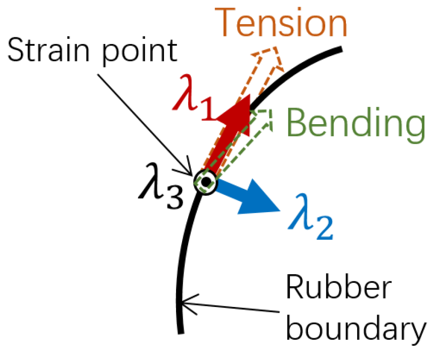
Here, ${\lambda }_1$,${\lambda }_2$ and ${\lambda }_3$ are the principal stretches (1 + principal extension) in three directions. As shown in Figure 2, the tension/compression and simple shear along the wall direction are mainly considered in the strain process of the sealing strip in this paper. Therefore, the main concern is the elongation along the wall, ${\lambda }_1$. The elongation perpendicular to wall thickness, ${\lambda }_2$, and the elongation along the extension direction of the sealing strip, ${\lambda }_3$, are set as equal, i.e., ${\lambda }_2={\lambda }_3$. The relationship between stress and strain is expressed by the following two formulas, Formula (13) is uniaxial tension or compression, and Formula (14) is simple shear:

$$\frac{\sigma }{{\lambda }_1-{\lambda }_1{}^2}=2C_{01}+\frac{2}{{\lambda }_1}{C}_{10}$$

(13)

$$\frac{\mathsf{\tau }}{\mathsf{\gamma }}=2C_{01}+2C_{10}$$

(14)

Here, $\sigma$ is the strain stress, τ is the shear stress and $\mathsf{\gamma }=\sqrt{I_1-3}$ is the corresponding shear strain to invariant $I_1$.

It should be noted that ${\lambda }_1$ and ${\lambda }_2$ are defined according to the shape of the sealing strip section. Coordinate conversion is required when using Cartesian coordinates for calculation.

2.3. Immersed Boundary Method

In this paper, IBM is used to simulate the force feedback and motion of the elastic boundary after receiving the external force. The immersed boundary uses the Euler grid to describe the flow field and the Lagrange grid to describe the solid boundary. Its basic principle is shown in Figure 1. The force balance relationship between the two coordinates is shown in Formula (15):

$$\mathit{F}\left(\mathit{x},t\right)={\displaystyle \sum }{\mathit{F}}_{ib}\left({\mathit{X}}_k,t\right)\mathsf{\Phi }\left(\mathit{x}-{\mathit{X}}_k\right)$$

(15)

Here, $\mathit{F}\left(\mathit{x},t\right)$ is the Euler body density force and $\mathit{x}$ is the Euler coordinate with a fixed position. ${\mathit{F}}_{ib}\left({\mathit{X}}_k,t\right)$ is the Lagrangian force, $\mathit{X}$ is the motion node expressed in Lagrangian coordinates and the following $k$ means the specific node number. $\mathsf{\Phi }$ is Dirac’s delta function (16), and the specific expression of interpolation functions [39] is shown in Formula (17):

$$\mathsf{\Phi }\left(x,y\right)=\frac{1}{\Delta x^2}\varphi \left(\frac{x}{\Delta x}\right)\varphi \left(\frac{y}{\Delta x}\right)$$

(16)

$$\varphi \left(r\right)=\{\begin{array}{c}\frac{1}{8}\left(3-2\left|r\right|+\sqrt{1+4\left|r\right|-4r^2}\right), \left|r\right|\le 1\\ \frac{1}{8}\left(5-2\left|r\right|-\sqrt{-7+12\left|r\right|-4r^2}\right), 1<\left|r\right|\le 2\\ 0, otherwise\end{array}$$

(17)

Equation (15) represents the relationship between displacement and force balance inside and outside the moving boundary (IB) due to solid boundary deformation. In case of a fluid–structure interaction, the external force, $\mathit{F}$, on the boundary is the fluid force, which can be solved by LBM. In this paper, it also includes the force generated by the extrusion and friction between the rigid solid boundary and the elastic boundary. The internal force of the boundary is mainly stress. Next, a detailed derivation of these forces will be provided.

2.4. Force on Immersed Boundary

2.4.1. Internal Force

In the case studied in this paper, the immersed boundary internal force, ${\mathit{F}}_{ib}$, is mainly composed of mass force, ${\mathit{F}}_m$, and strain force, ${\mathit{F}}_s$. The two forces are discussed separately below.

(1) Mass force

Generally, the IB-LBM calculation example needs to consider that the mass is all solid inside the immersed boundary, and its internal mass effect is relatively complex. Fortunately, in the problem of this paper, the sealing strip is a thin-walled structure with negligible wall thickness, and both sides are the same fluid. Therefore, it is only necessary to concentrate the mass of the sealing strip on the immersion node and use the inertial force, ${\mathit{F}}_m$, as shown in Equation (18):

$${\mathit{F}}_m\left({\mathit{X}}_k\right)=-m_k{\mathit{a}}_k$$

(18)

Here, $m_k$ represents the equivalent mass of each node and ${\mathit{a}}_k$ is the acceleration of the node.

(2) Strain force

For hyper-elastic materials, the strain force, ${\mathit{F}}_s$, can ignore the effects of viscosity and plasticity, and the contribution of the total strain energy, $W,$ can usually be written as,

$$W=W_t+W_b+W_{\mathit{a}}+W_v$$

(19)

where $W_t$ is the tensile force term, $W_b$ is the bending force term, $W_{\mathit{a}}$ is the surface force term and $W_v$ is the volume force term. In the case of this paper, the forces caused by surface tension and volume change of materials are very small and can be ignored, so only tension, $W_t$, and bending, $W_b$, are considered. The relationship between stress and strain energy is as described in Formula (20):

$${\mathit{F}}_s=-\frac{\partial W\left(\mathit{X}\right)}{\partial \mathit{X}}$$

(20)

According to Formulas (13) and (14), the tensile force, ${\mathit{F}}_t$, and bending force, ${\mathit{F}}_b$, are obtained as:

$${\mathit{F}}_t=2k_t\left[C_{01}\left({\lambda }_1-\frac{1}{{\lambda }_1^2}\right)+\frac{C_{10}}{{\lambda }_1}\left({\lambda }_1-\frac{1}{{\lambda }_1^2}\right)\right]$$

(21)

$${\mathit{F}}_b=\left(C_{01}+C_{10}\right)k_t\sqrt{{\lambda }_1^2+\frac{2}{{\lambda }_1}-3}$$

(22)

In the IB method, the elastic boundary can only be represented by one layer of the IB grid, so the wall thickness must be corrected. The wall thickness correction factor, $k_t$, is determined by the ratio of the thickness of the actual boundary to the thickness of the IB. In this paper, it is assumed that the thickness of the IB is equal to the LBM lattice size, and $k_t$ is calculated by Equation (23):

$$k_t=\frac{\delta }{\Delta x}$$

(23)

Here, $\delta$ is the actual wall thickness of the elastic boundary. The total elastic strain force, that is, the internal force at the IB, ${\mathit{F}}_s$, is the sum of tensile force, ${\mathit{F}}_s$, and bending force, ${\mathit{F}}_b$,

$${\mathit{F}}_s={\mathit{F}}_b+{\mathit{F}}_t$$

(24)

Through the above method, the mechanical properties of the sealing strip can be described by the immersed boundary. It should be noted that all variables and forces described in this section are in Lagrangian form and need to be converted to Euler form for use in the control fluid equation.

2.4.2. External Force

In this paper, the immersed boundary node representing the sealing strip may not only contact with the fluid, but also squeeze and friction with the rigid wall. These are two different situations, which will be discussed separately later. In order to distinguish the two cases of nodes, we add a letter after the subscript $k$ of the node, where $kf$ indicates that the node is in contact with fluid and $ks$ indicates that the node is in contact with a solid.

(1) With fluid

When the immersed boundary node is surrounded by fluid, the velocity and force of fluid could be calculated by LBM, as introduced in Section 2.1. Since the fluid is viscous, the IB must meet the no-slip condition (25):

$$\mathit{u}\left({\mathit{X}}_{kf}\right)={\mathit{U}}_{kf}$$

(25)

Here, ${\mathit{U}}_{kf}$ is the boundary velocity and $\mathit{u}\left({\mathit{X}}_{kf}\right)$ represents the fluid velocity at the boundary.$\mathit{u}\left({\mathit{X}}_{kf}\right)$ can be obtained by interpolating the velocity, $\mathit{u}\left(\mathit{x}\right)$, of Euler points around ${\mathit{X}}_{kf}$, as shown in Equation (26):

$$\mathit{u}\left({\mathit{X}}_{kf},t\right)={\displaystyle \sum }\mathit{u}\left(\mathit{x},t\right)\mathsf{\Phi }\left(\mathit{x}-{\mathit{X}}_{kf}\right)$$

(26)

When the IB velocity, ${\mathit{U}}_{kf}$, is obtained, the position of the next IB point can be calculated by (27):

$${\mathit{X}}_{kf}\left(t+\Delta t\right)={\mathit{X}}_{kf}\left(t\right)+{\mathit{U}}_{kf}\Delta t$$

(27)

(2) With solid

When the immersed boundary coincides with the rigid solid boundary, that is, the elastic solid boundary contacts and squeezes with the rigid solid boundary, the boundary is constrained by non-deformable and friction coefficient conditions.

When the IB contacts with the rigid boundary, the rigid boundary limits the displacement of the immersed boundary, and the immersed boundary can only adapt to the rigid boundary through deformation.

$${\mathit{U}}_{ks,n}\le 0$$

(28)

where n represents the normal direction of the vertical boundary. The force, ${\mathit{F}}_s$, generated by the boundary strain is still calculated, as introduced in Section 2.4.1.

Since the two solid boundaries are tangent, only the normal force, ${\mathit{F}}_b$, inside the immersed boundary and the applied normal force, ${{\mathit{F}}^{\prime }}_n$, are in the same axial direction, and ${{\mathit{F}}^{\prime }}_n$ can be interpolated by distance with ${\mathit{F}}_b$ of two adjacent immersed boundary nodes.

$${{\mathit{F}}^{\prime }}_n\left(x,t\right)={\mathit{F}}_b\left({\mathit{X}}_{k{s}^{\prime }},t\right)\frac{\left(x-{\mathit{X}}_{k{s}^{″}}\right)}{\Delta x}+{\mathit{F}}_b\left({\mathit{X}}_{k{s}^{″}},t\right)\frac{\left(\mathit{x}-{\mathit{X}}_{k{s}^{\prime }}\right)}{\Delta x}$$

(29)

Here, ${\mathit{X}}_{k{s}^{\prime }}$ and ${\mathit{X}}_{k{s}^{″}}$ represent two immersed boundary nodes adjacent to solid boundary node $x$. In fact, when the elastic boundary contacts with the rigid boundary, it receives the constraint of the rigid boundary in the normal direction. No matter how large ${{\mathit{F}}^{\prime }}_n$ is, the rigid wall will produce a reaction force to counteract it and will not move to the other side. The purpose of calculating ${{\mathit{F}}^{\prime }}_n$ is to calculate the friction, ${{\mathit{F}}^{\prime }}_{\tau }$, between two boundaries. When there is a tangential movement trend of the immersed boundary and ${{\mathit{F}}^{\prime }}_n\left(x,t\right)>0$, the friction is calculated by Formulas (30) and (31):

$${{\mathit{F}}^{\prime }}_{\tau }\left(x,t\right)=-{\mu }_0{{\mathit{F}}^{\prime }}_n\left(x,t\right)$$

(30)

$${{\mathit{F}}^{\prime }}_{\tau }\left(x,t\right)=-{\mu }_1{{\mathit{F}}^{\prime }}_n\left(x,t\right)$$

(31)

Here, ${\mu }_0$ is the static friction coefficient, ${\mu }_1$ is the dynamic friction coefficient and the negative sign indicates that the direction of the force is opposite to the direction or trend of motion.

2.5. Iterative Algorithm

In time step $t_0$, the immersed boundary nodes’ position, ${\mathit{X}}_k\left(t_0\right)$, velocity, ${\mathit{U}}_k\left(t_0\right)$, acceleration, ${\mathit{a}}_{\mathit{k}}\left(t_0\right)$, boundary internal force, ${\mathit{F}}_{ib}\left({\mathit{X}}_k,t_0\right)={\mathit{F}}_m\left({\mathit{X}}_k,t_0\right)+{\mathit{F}}_s\left({\mathit{X}}_k,t_0\right)$, and fluid state,$\mathit{u}\left(\mathit{x},t_0\right)$, $\rho \left(\mathit{x},t_0\right)$, are known. The iterative calculation can be carried out according to the following steps:

• According to acceleration, ${\mathit{a}}_{\mathit{k}}\left(t_0\right)$, calculate and update inertial force, ${\mathit{F}}_m\left({\mathit{X}}_k,t_1\right)$.
• Judge the state of immersed boundary nodes: mark the nodes whose own and adjacent nodes coincide with the rigid boundary as ${\mathit{X}}_{ks}\left(t_0\right)$, and the other nodes as ${\mathit{X}}_{kf\left(t_0\right)}$.
• Calculate stress, ${\mathit{F}}_s\left({\mathit{X}}_{kf},t_1\right)$, of immersed boundary nodes in contact with fluid by the method introduced in Section 2.4.1.
• Update the internal force of the boundary node with fluid immersion, which is the sum of inertial force and strain force, ${\mathit{F}}_{ib}\left({\mathit{X}}_{kf},t_1\right)={\mathit{F}}_s\left({\mathit{X}}_{kf},t_1\right)+{\mathit{F}}_m\left({\mathit{X}}_{kf,}{t}_1\right)$.
• Through the adjacent nodes, the internal force, ${\mathit{F}}_{ib}\left({\mathit{X}}_{kf},t_1\right)$, of nodes in contact with fluid is transmitted to nodes in contact with a solid, ${\mathit{X}}_{ks}$.
• Judge the friction state of ${\mathit{X}}_{ks}$ nodes: when ${\mathit{F}}_t\left({\mathit{X}}_{ks},t_1\right)>{\mu }_0{\mathit{F}}_b\left({\mathit{X}}_{ks},t_1\right)$, it is a static friction state, and when ${\mathit{F}}_t\left({\mathit{X}}_{ks},t_1\right)\le {\mu }_0{\mathit{F}}_b\left({\mathit{X}}_{ks},t_1\right)$, it is a dynamic friction state. In the static friction state, ${\mathit{U}}_{ks}\left(t_1\right)=0$. In the dynamic friction state, calculate ${\mathit{a}}_{\mathit{k}\mathit{s}}\left(t_1\right)$ and ${\mathit{U}}_{ks}\left(t_1\right)$ by ${\mathit{F}}_t\left({\mathit{X}}_{ks},t_1\right)+{\mu }_1{\mathit{F}}_b\left({\mathit{X}}_{ks},t_1\right)+{\mathit{F}}_m\left({\mathit{X}}_{ks},t_1\right)=0$.
• According to Formulas (29), (30) and (31), external force, ${\mathit{F}}^{\prime }\left(\mathit{x},t_1\right)$, could be obtained: the normal part ${{\mathit{F}}^{\prime }}_n\left(x,t_1\right)$ offsets the rigid wall, the tangential force, ${{\mathit{F}}^{\prime }}_{\tau }\left(x,t_1\right)$, is corrected for the tensile force, ${\mathit{F}}_t\left({\mathit{X}}_{ks},t\right)$, and transmitted to the nodes, ${\mathit{X}}_{kf}$, which are in contact with the fluid.
• According to the internal force of the immersed boundary after friction correction, ${\mathit{F}}_{ib}\left({\mathit{X}}_{kf},t_1\right)$, the physical force of the immersed boundary to the fluid, $\mathit{F}\left(\mathit{x},t_1\right)$, can be obtained through Equation (15).
• Calculate the new fluid state, $\mathit{u}\left(\mathit{x},t_1\right)$ and $\rho \left(\mathit{x},t_1\right)$, by $\mathit{F}\left(\mathit{x},t_1\right)$ and the inlet boundary condition using LBM.
• According to the no-slip constraint (25) and Equation (26), update the motion velocity of the immersed boundary node, ${\mathit{U}}_{kf}\left(t_1\right)$.
• According to the time step $\Delta t$ and the velocity ${\mathit{U}}_{kf}\left(t_1\right)$, calculate nodes’ position, ${\mathit{X}}_{kf}\left(t_1\right)$, and acceleration, ${\mathit{a}}_{kf}\left(t_1\right)$.

So far, ${\mathit{X}}_k\left(t_0\right)$, ${\mathit{U}}_k\left(t_0\right)$,${\mathit{a}}_{\mathit{k}}\left(t_0\right)$, ${\mathit{F}}_m\left({\mathit{X}}_k,t_0\right)$, ${\mathit{F}}_s\left({\mathit{X}}_k,t_0\right)$, $\mathit{u}\left(\mathit{x},t_0\right)$ and $\rho \left(\mathit{x},t_0\right)$ are all updated to the value at time $t_1$. Increase the time step to $t_2=t_1+\Delta t$, then repeat steps 1–11.

3. Modeling and Verification

3.1. Sealing System Model

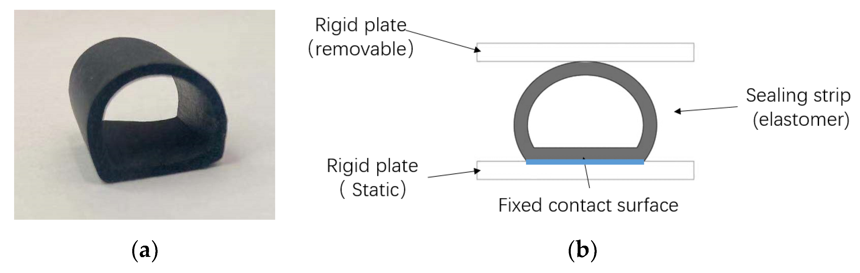
The specific object of this paper is the D-shape hollow sealing strip, as shown in Figure 3a. The sealing strip is extruded by abrasive tools and has the same span-wise direction. Therefore, this paper only studies the fluid–structure interaction problem of the sealing strip in the 2D plane. In the uncompressed state, the geometric dimensions of the sealing strip are as follows: the height $h_s=$11 mm, the maximum width $w_{m\mathit{a}x}=$15.8 mm and the wall thickness $\delta =$ 1.5 mm. The thickness of the sealing strip is very uniform, and the ratio between the wall thickness and the overall size is small. Therefore, it is reasonable to describe the sealing strip with the immersed boundary in this paper. According to Rivlin’s model, the material properties of the sealing strip are $C_{01}$= 0.8706 MPa and $C_{10}$= 0.044 MPa. In practical use, the straight edge is pasted on the solid wall with great stiffness, so it can be considered that this edge is not displaceable and deformable in subsequent modeling.

The 2D FEM model used to verify IB-LBM is shown in Figure 3b, including the elastic part according to the actual sealing strip geometry, the lower rigid plate fixedly connected with the sealing strip and the upper plate that can move up and down to simulate extrusion.

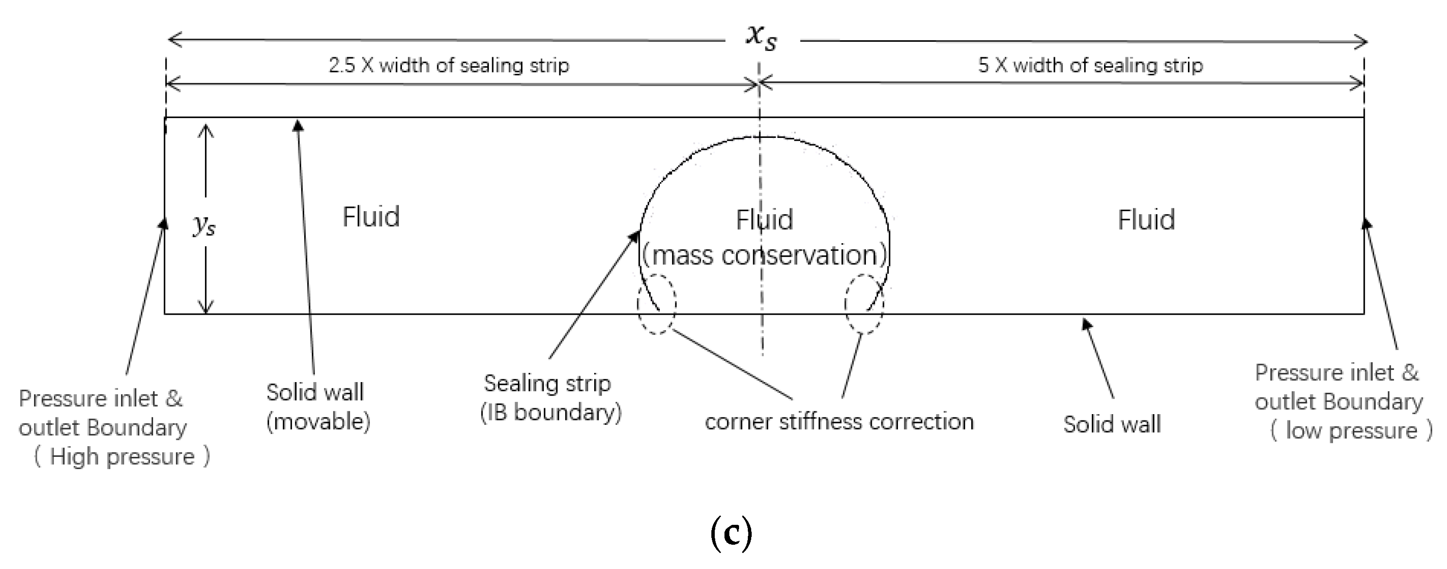
The IB-LBM model used in this paper is shown in Figure 3c. The height of the calculation domain, $y_s$, is determined by the height of the sealing strip, $h_s$, and the preloading shrinkage, $p_c$. The length of the calculation domain, $x_s$, is 7.5 times of the width of the sealing strip, $w_{m\mathit{a}x}$. The flow on the high-pressure side is more stable, while the separated flow on the low-pressure side is more complex. In order to avoid the interference of the outlet boundary, the length of the low-pressure part is longer.

The curved edge of the sealing strip was described by a layer of IB. The thickness of the sealing strip was ignored, and $C_{01}$, $C_{10}$ and $k_t$ were used to simulate the actual physical properties, which proved to be feasible by subsequent verification.

The straight edge of the sealing strip is fixedly connected with the rigid wall, so it will be ignored in the modeling process. In addition, this straight edge indirectly improves the stiffness of the curved edge near the corner by increasing $C_{01}$ and $C_{10}$ of the IB from ground to 2$\delta$ height for “corner stiffness correction”.

The top and bottom of the sealing strip are two straight lines representing the rigid boundary, which are set as the no-slip boundary in LBM. The upper wall simulates the moving boundary of the extruded sealing strip through displacement and force, and its displacement is the preloading shrinkage, $p_c$.

Both ends are non-equilibrium extrapolation scheme pressure inlet and outlet boundaries [40,41], and the pressure difference on both sides of the sealing strip can be adjusted by setting two boundary pressure values.

The whole computational domain, including the inside and outside of the sealing strip, was filled with the same kind of fluid. The internal fluid is mass conserved. In cases of this paper, the fluid object studied was air, and the subsequent fluid properties were set as air.

3.2. Simulation Steps

In this paper, IB-LBM is used to simulate the fluid–structure interaction of a pre-compressed hollow sealing strip under the action of differential pressure, which mainly includes four major steps, as described below.

3.2.1. Modeling

First, the attributes and geometric positions of each boundary were determined according to the model described in Figure 2c. In order to accurately describe the positional relationship between the sealing strip and the outflow field and the rigid boundary, the immersed boundary was selected as the outer boundary of the actual sealing strip geometry.

Next, relevant physical parameters were set, including: fluid density and viscosity expressed by lattice kinematic viscosity, $v_l$, density of sealing strip, ρ, and wall thickness, δ, expressed by lattice mass, $m_l$, stress properties of materials $C_{01}$ and $C_{10}$, thickness correction factor, $k_t$, and friction coefficient between solid boundaries ${\mu }_0$ and ${\mu }_1$.

3.2.2. Meshing

After the physical properties were set, the square complementary grid was used to establish the calculation domain. In this paper, both $\Delta x$ and $\Delta t$ were dimensionless to 1 unit in order to simplify the calculation.

When setting the lattice number, $N$, in the characteristic length direction, it was ensured that the lattice Reynolds number was consistent with the actual Reynolds number. See Equation (32) for the lattice Reynolds number and Equation (33) for the actual Reynolds number:

$$R{e}_l=\frac{u_{l}N}{v_l}$$

(32)

$$Re=\frac{uL}{\upsilon }$$

(33)

where $u_l$ is the lattice flow velocity, ${\upsilon }_l$ is the lattice kinematic viscosity, $u$ is the flow velocity, $L$ is the characteristic length, that is, the height, $y_s$, of the calculation domain, and $\upsilon$ is the kinematic viscosity of the fluid.

In addition, in order to ensure the computational stability of LBM, the lattice kinematic viscosity, ${\upsilon }_l$, and relaxation time, ${\tau }_l$, were determined by Equation (34), and the lattice flow velocity, $u_l$, was determined by Equation (35):

$${\upsilon }_l=\frac{{\tau }_l-0.5}{3}>0.0001$$

(34)

$$u_l<0.2$$

(35)

3.2.3. Pre-Compression

In the process of pre-compression simulation, the initial value of fluid velocity was set to zero, and the pressures at the inlet, outlet and inside the sealing strip on both sides were set to be equal.

Pre-compression is achieved by gradually lowering the coordinates of the upper rigid boundary. After each grid is moved, the IB-LBM iteration with large steps was carried out to gradually complete the compression process. When the set preloading shrinkage, $p_c$, is reached, calculate the residual position of the sealing strip boundary, ε, according to Formula (36):

$$\epsilon ={\displaystyle \sum }\sqrt{{\left(x\left(X_k,t+\Delta t\right)-x\left(X_k,t\right)\right)}^2+{\left(y\left(X_k,t+\Delta t\right)-y\left(X_k,t\right)\right)}^2}$$

(36)

When residual $\epsilon <1\times {10}^{-5}$, it can be considered that the deformation of the sealing strip is in a stable state. Maintain the strain state of the sealing strip, including the position of the immersed boundary, ${\mathit{X}}_k$, and the stress, ${\mathit{F}}_s$. The global velocity of the flow field, $\mathit{u}\left(\mathit{x},t_0\right)$, was initialized to zero.

3.2.4. Pressure Difference Loading

In this paper, the pressure difference on two sides of the sealing strip was simulated by adjusting the pressure at the inlet and outlet, which was specifically set to keep the pressure at the low-pressure end stable and increase the pressure at the high-pressure end. When the instantaneous change of inlet pressure is large, a phenomenon similar to a “shock wave” will occur. In order to reduce the impact effect caused by pressure change, the cosine function tangent to the extreme values on both sides of the curve was used to decompose the pressure and gradually increase the pressure to the set target value. When the pressure difference reached the target value, the pressure values of the pressure inlet and outlet were kept stable, and then the iterative calculation continued until complete simulation results were obtained.

3.3. Model Validation

Although the traditional finite element method cannot simulate the whole process of seal strip failure, the static failure process of seal strip deformation to notch and flow can be accurately simulated when the seal has not failed, that is, the pressure on both sides remains independent.

In this paper, the finite element method was used to simulate the boundary deformation process of the sealing strip under the condition of stable pressure on both sides, including “solid boundary pre-compression” and “sealing deformation under fluid pressure”, which was used to verify the IB-LBM model.

In the finite element simulation, Abaqus (Version 2019_09) was used for the simulation, which is accurate in nonlinear finite element simulations. The sealing strip was divided into quadrilateral grids with a grid size of 0.1 mm and total grid number of 7778, and simulation accuracy reached ${10}^{-3}$ mm, which can meet the requirements of grid independence.

Here, IB-LBM is only used to observe the deformation of IB under the action of uniform force, and it does not involve flow field analysis. Therefore, it is not necessary to meet the Reynolds number requirements described in Equations (32) and (33). The grid size of LBM was set to 0.1 mm, which was consistent with the finite element method.

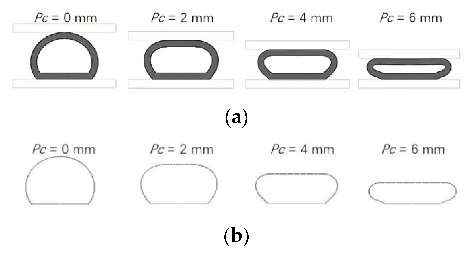
When the fluid pressure on both sides is the same, the process of pre-compression of the sealing strip by the rigid body boundary is as shown in Figure 4. The pre-compression amount is represented by $p_c$. It can be seen that the shape obtained by IB-LBM and FEM is very similar.

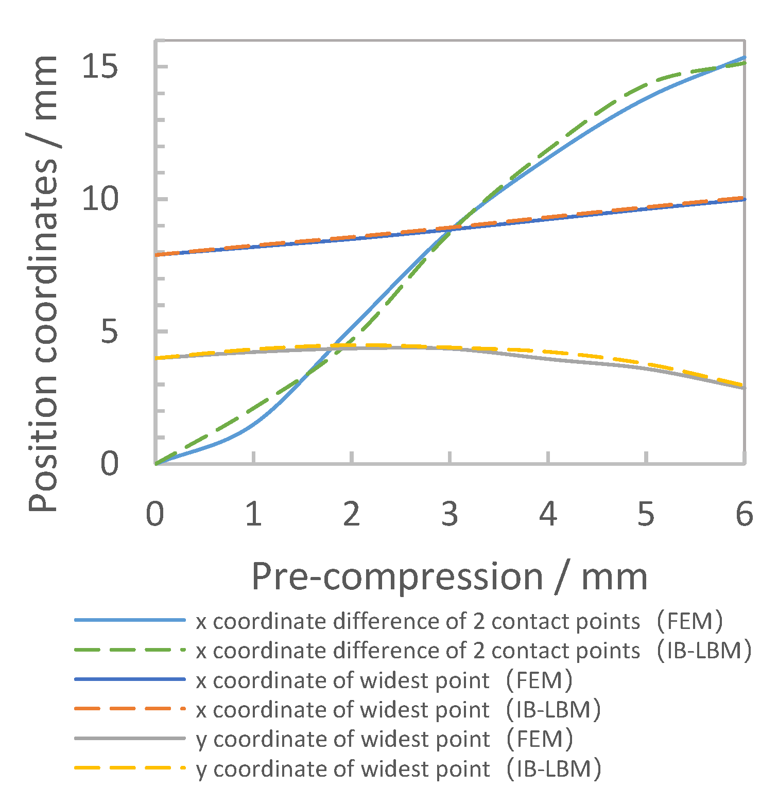
The quantitative analysis results of the pre-compression deformation of the sealing strip are shown in Figure 5. The coordinate difference between the starting point and ending point of the contact part means the effective contact width of the sealing strip and upper boundary, which ignores the separation of the contact part due to the twisted concave of the sealing strip. The coordinate of the widest point is an intuitive and effective way to describe the bending deformation on sides of the sealing strip. The results show that the coordinates obtained by the two methods are in good agreement.

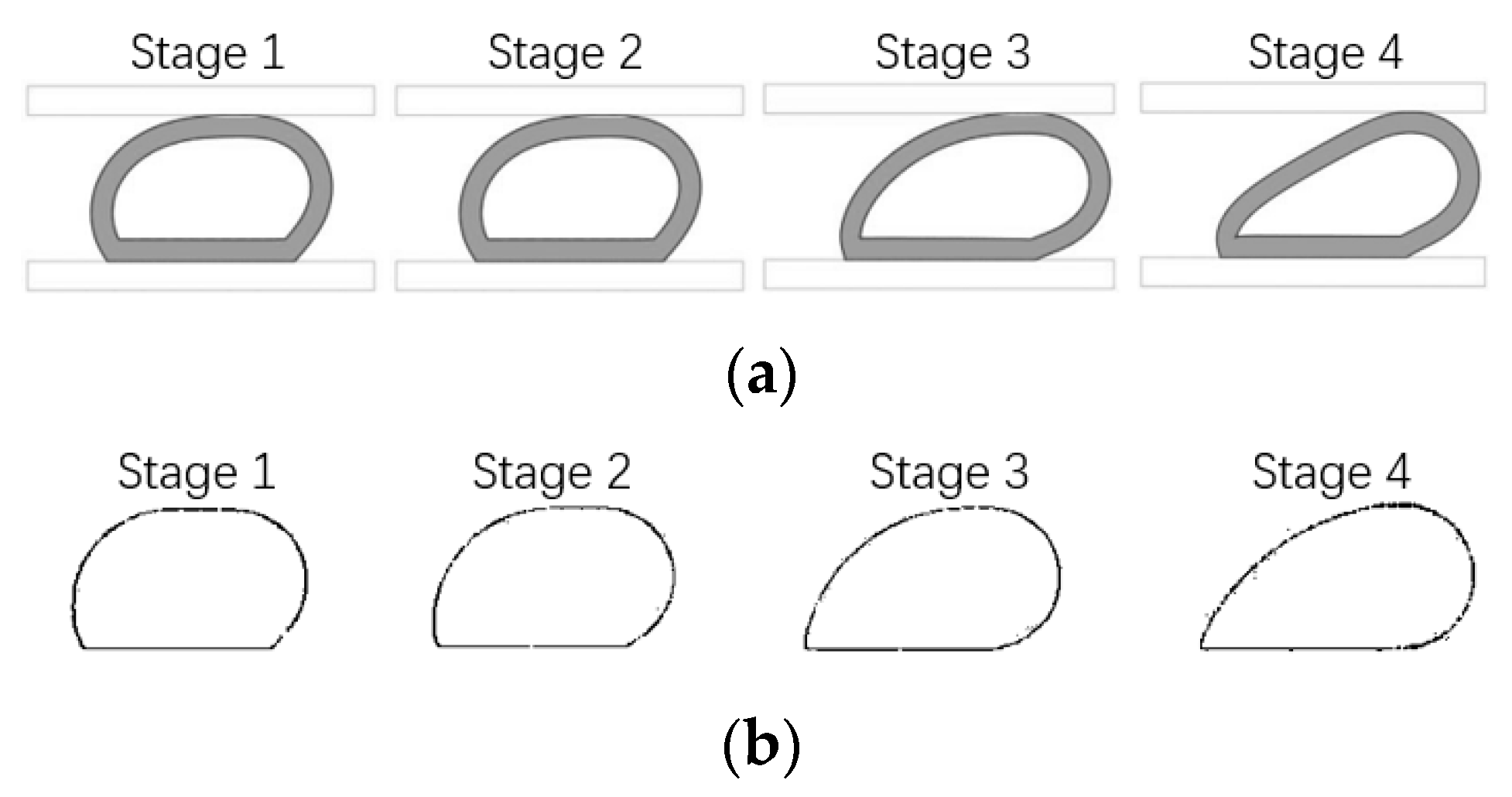
After 1 mm pre-compression, the deformation results under the action of pressure difference are shown in Figure 6. The setting of FEM is to apply a pressure load consistent with IB-LBM on the left side of the sealing strip. At the same time, considering the increase of internal cavity pressure caused by the change of internal cavity volume during the compression of the sealing strip, the pressure load compensation is carried out inside the sealing strip.

In Figure 6, stage 1 is the moment when the sealing strip begins to deform after pressure loading, stage 2 is the intermediate process of deformation and stage 3 is the moment of critical failure. In these three stages, the results of the two methods are very close, which verifies the effectiveness of IB-LBM. Stage 4 is the case in which the seal has failed, and there is a small gap between the sealing strip and the upper wall. In the IB-LBM simulation, air flow has passed through the gap from the high-pressure side to the low-pressure side. With the increase of speed, the pressure on the left side of the sealing strip decreases. FEM cannot simulate the pressure reduction loaded on the side, so the relative deformation is more intense and obviously distorted.

4. Analysis of Results

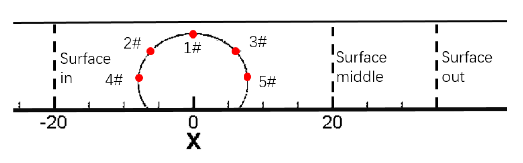
In this section, the simulation results of the fluid–structure interaction of the sealing strip will be analyzed in detail. As shown in Figure 7, five position monitoring points, which represented by “1# ~ 5#”, were set on the immersed boundary to observe the time history of seal strip deformation. In addition, three detection surfaces were set upstream and downstream of the seal strip to record the flow field information, such as total flow and total vorticity, on the surface to judge the macro-movement of the flow field.

There are many variable parameters, such as the pressure difference of the two sides, physical properties of fluid, physical properties of sealing strip, initial pre-compression amount and so on. Here, we kept the physical properties of the sealing strip, which were, shape, thickness correction factor, $k_t$, $C_{01}$,$C_{10}$ and mass, $m_k$, completely consistent with the real object. When setting the fluid properties, the fluid density was set to be consistent with the air to ensure that the inertia force between the fluid and the sealing strip was similar. Under the above conditions, by adjusting the differential pressure, $\mathsf{\delta }p$, and the pre-compression amount, $p_c$, three typical cases of the coupling between the sealing strip and the differential pressure flow field were obtained.

4.1. Sealing Non-Fail

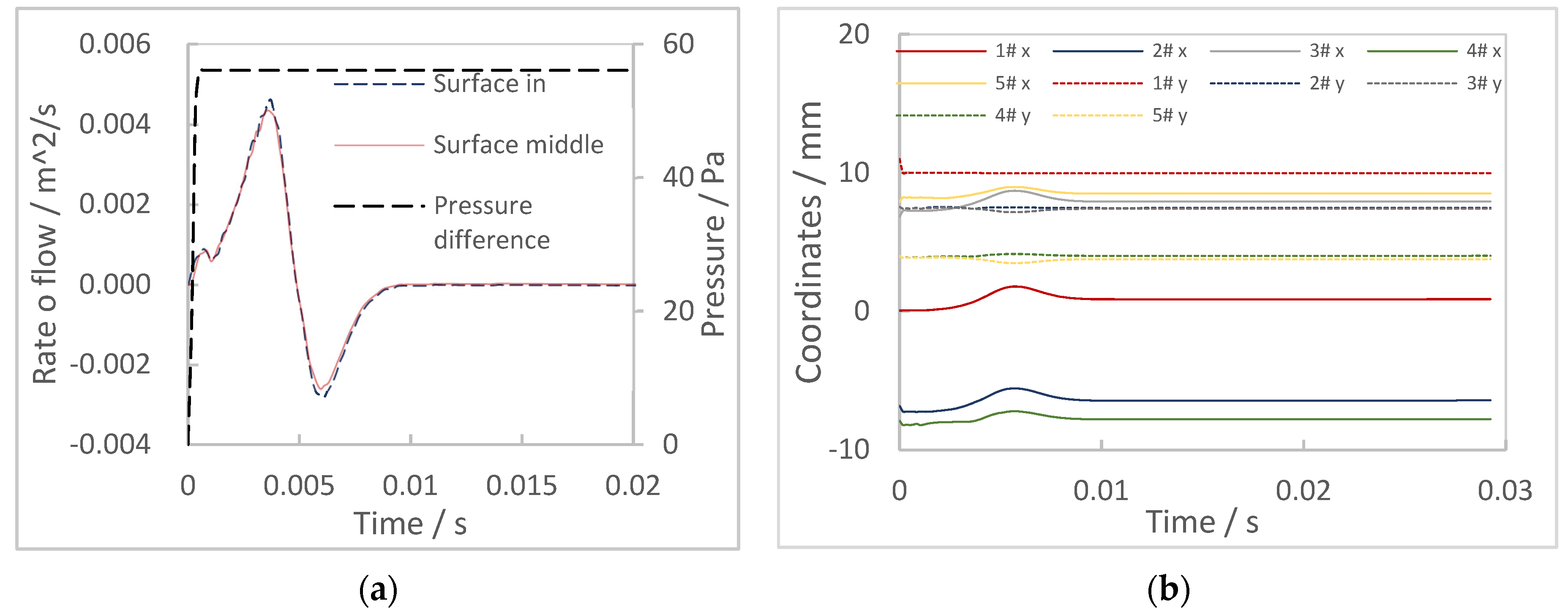
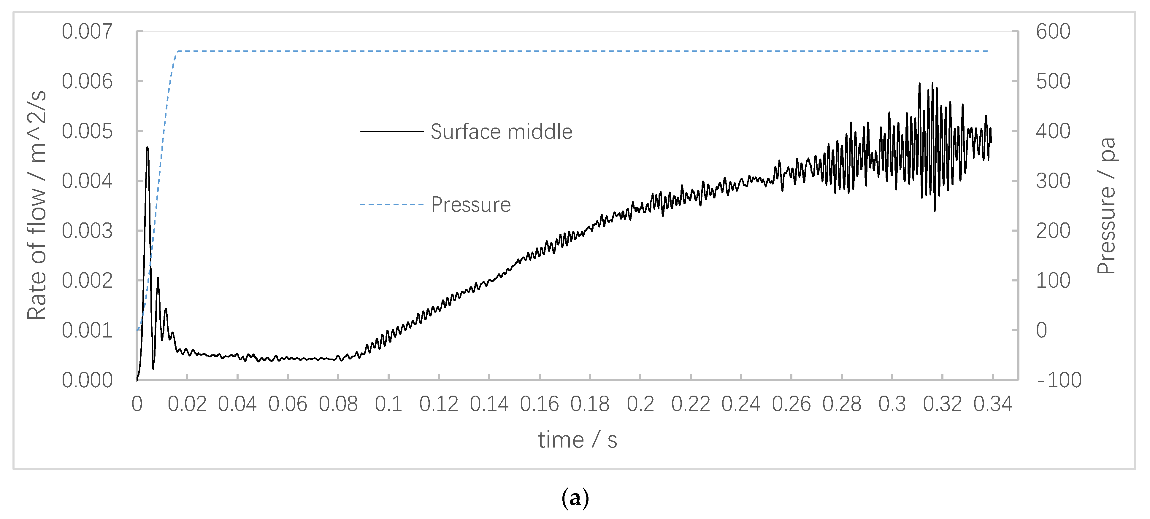
Firstly, a simplest case is presented. When the pressure difference is small ($\mathsf{\delta }p=55\mathrm{Pa}$) and the sealing strip has a sufficient pre-compression amount ($p_c=1\mathrm{mm}$), the sealing strip will not fail. We call it the “sealing non-failure” condition. Figure 8 shows the time-varying results of loading pressure, flow on two sides of the sealing strip and the position of the sealing strip under this condition. The results in Figure 8a show that with the pressure loading, the flow in the tunnel first increases significantly, then quickly falls back to the negative range after reaching the peak in about 0.0036 s, and finally, falls back to near zero. Combined with the displacement of the sealing strip shown in Figure 8b, it could be known that the sealing strip deforms towards the low-pressure end under the action of pressure difference, and then rebounds. The above situation is further confirmed by the sealing strip position and velocity field cloud diagram shown in Figure 9.

4.2. Sealing Absolute Fail

Next, another common case is presented. When the pre-compression amount of the sealing strip is negative ($p_c=-1\mathrm{mm}$), the sealing strip is always in the failure state regardless of the pressure difference ($\mathsf{\delta }p=550\mathrm{Pa}$), which is called the “sealing absolute failure” condition. This case usually occurs when the vehicle is running at high speed, the door is sucked out, or there is a problem with the locking device of the pressure vessel. In order to compare with the similar flow not in the FSI state, the “steady” geometry of the seal strip after failure under pressure was selected as a rigid boundary, then simulated by LBM. In both cases, the Reynolds number is about 2000.

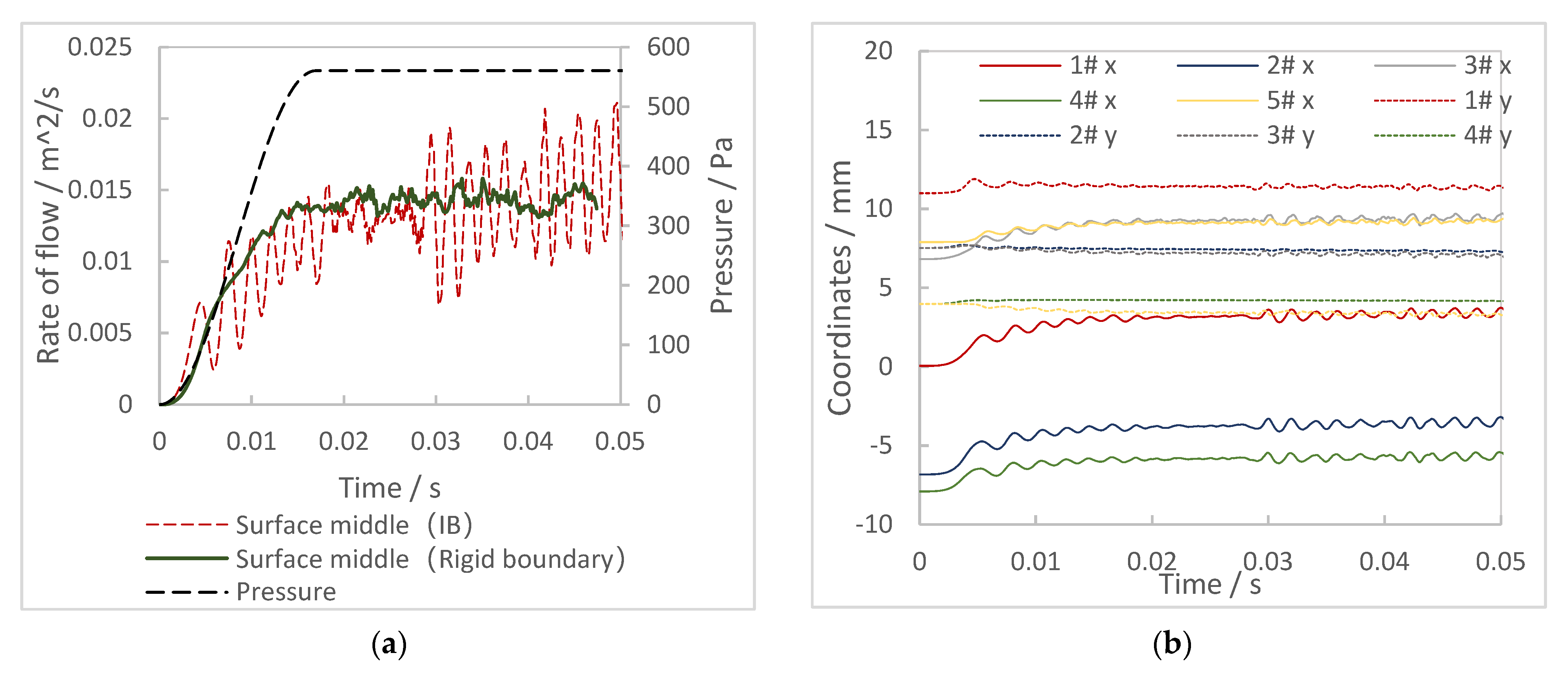
The results in Figure 10a show that with the pressure loading, the flow in the pipeline increases. After the pressure difference reaches the maximum value, the flow gradually enters a relatively stable state, with an average value of about 0.14 m²/s. There are also obvious differences between the two cases. In the results of the fixed boundary simulation, the fluctuation in the process of flow rise is very small, and there is only a small amplitude with non-periodic fluctuation after reaching the stabilization stage. In the results of the fluid–structure interaction simulation, the flow has obvious periodic fluctuation in the rising process, and the frequency is about 430 Hz. After the pressure reaches the maximum value, the flow fluctuates irregularly in a small amplitude within 0.008 s, and then begins to fluctuate in a large period, with a frequency of about 505 Hz. Combined with the results of seal strip displacement in Figure 10b, in the third stage, the frequency of velocity fluctuation is completely consistent with displacement fluctuation of the sealing strip in the x-direction. Therefore, the change of flow is closely related to the deformation and jitter of the sealing strip.

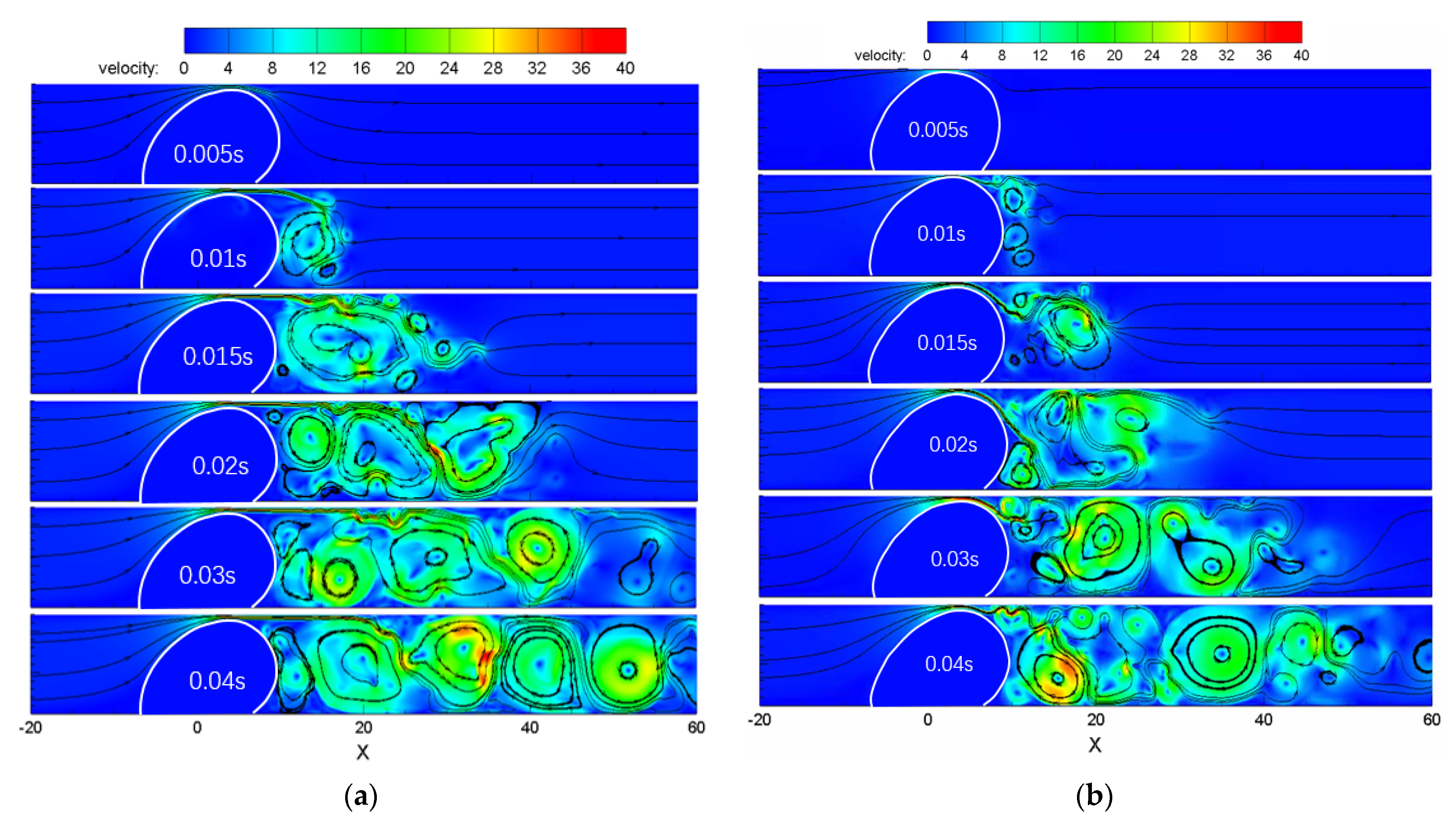
Next, the specific flow field was analyzed through the velocity cloud diagram and streamlined, as shown in Figure 11. In general, the flow fields of the two cases are relatively similar: they are separated following the slit that occurs between the sealing strip and the upper wall, form a vortex, then gradually enhance in the process of moving downstream.

In the case of the fixed wall, as shown in Figure 11a, the vortex is formed due to the shear structure of velocity. When the scale of the vortex increases to be limited by the pipeline, it begins to accelerate downstream, and then a new vortex will be formed. In this case, the overall scale of the vortex moving downstream is equivalent to the size of the channel.

In the case of FSI, as shown in Figure 11b, the vortex formation is not only affected by the instability of the shear layer, but more importantly, the position of the high-speed wall-attached jet is constantly moving with the boundary of the sealing strip shaking back and forth, resulting in the interruption of the vortex scale by the external injection flow before it reaches maximum size, forming a new vortex. In short, the size of the vortex varies greatly, which is different from that of the fixed wall. Combined with the results in Figure 10a, it can be considered that the fluid–structure interaction effect greatly interferes with the flow field, whether it is the overall flow or the local vortex structure.

4.3. Sealing Dynamic Fail

Finally, the most complex case is presented. The sealing strip has a certain pre-compression amount ($p_c=1\mathrm{mm}$), and the pressure difference is relatively large ($\mathsf{\delta }p=500\mathrm{Pa}$). The sealing strip originally in contact with the wall is constantly deformed under the action of pressure, and then a channel is formed between the sealing strip and the wall, resulting in flow. We call it the “sealing dynamic fail” condition. The Reynolds number of this case is about 600.

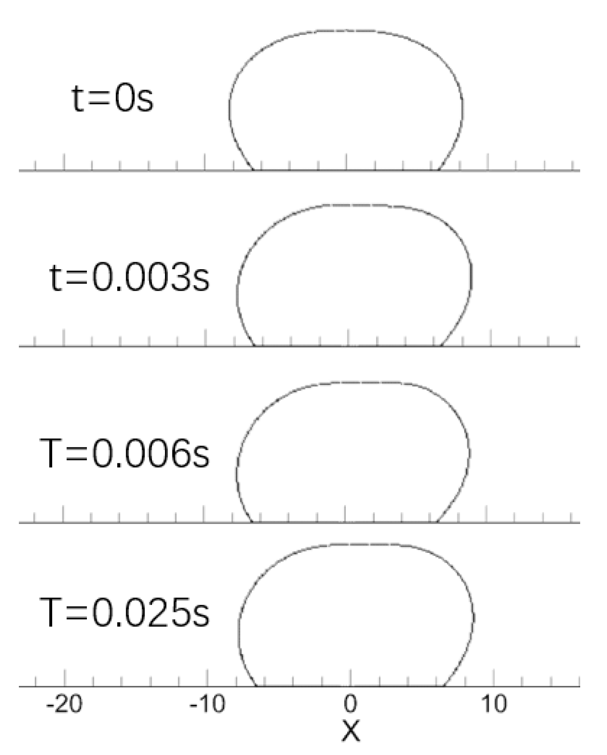
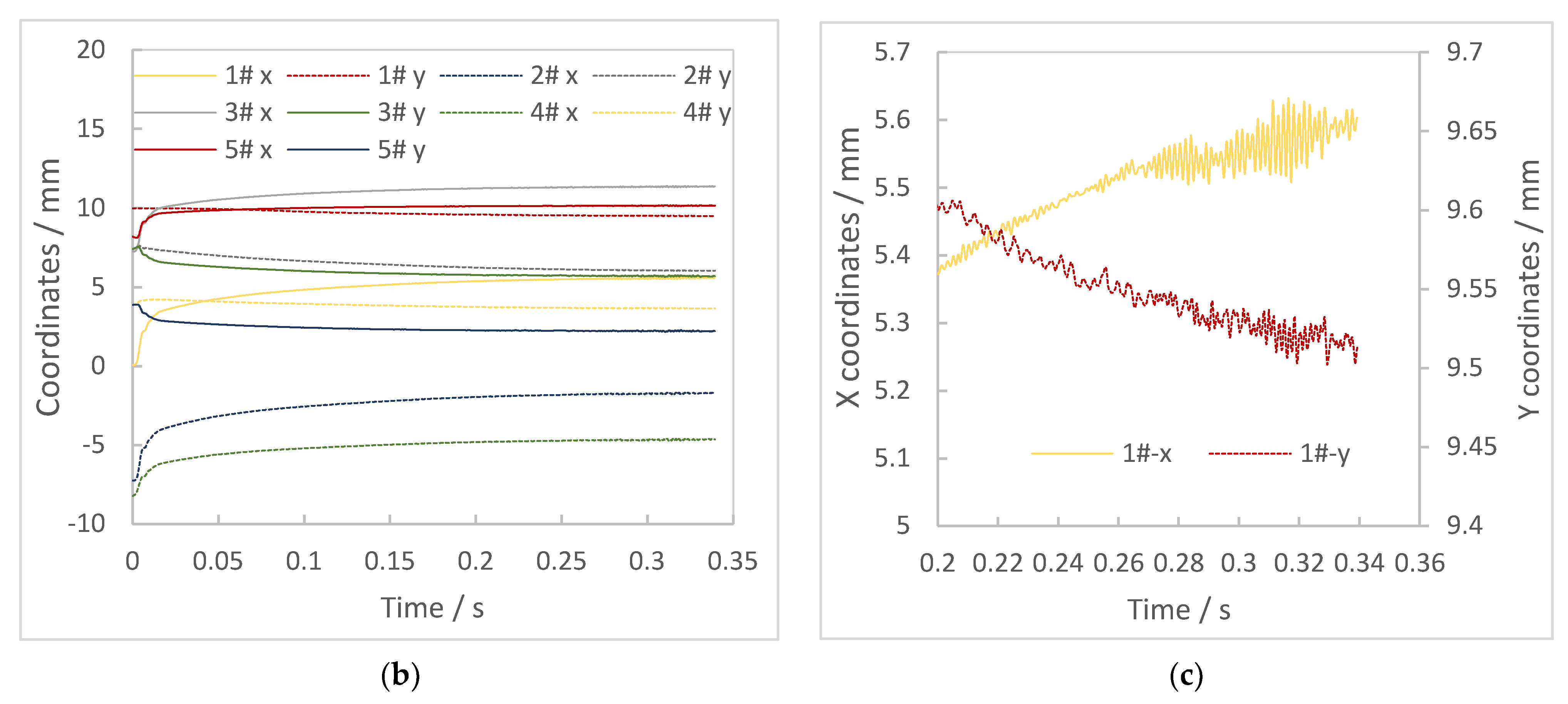
As shown in the time domain results of Figure 12, this case could be divided into four stages according to the flow. The first stage is about 0~0.02 s. With the pressure loading, the sealing strip produces a large overall displacement and then rebounds. At the same time, there is a corresponding flow in the flow field. The displacement of the sealing strip tends to equilibrium after several oscillations, and the flow rate also decreases to very small. In this process, the sealing strip is still in contact with the upper wall. The shape and flow field of the sealing strip in the first stage are very similar to the “non-failure” case.

The second stage is about 0.02~0.09 s. At this stage, the sealing strip continues to deform under pressure, and the coordinates of the contact point with the wall continue to move backward. However, the seal is still not working under this condition, so the overall flow rate keeps a very small state. The second stage can be regarded as an excessive state.

The third stage is about 0.09~0.27 s. At the beginning of this stage, the sealing strip reaches the critical state, and the gap between the sealing strip and the wall increases continuously. The flow then rises in small fluctuations.

The fourth stage is the time period after 0.27 s. The deformation of the sealing strip reaches the state of dynamic balance. The average displacement increases very slowly, and the fluctuation degree also increases. The flow also began to pulsate sharply. Overall, the fourth stage is very similar to the “absolute failure” case, but the third stage, as an intermediate transition state, is quite different from the rising process of the “absolute failure” case. In the third stage of the dynamic failure process, the overall displacement of the seal strip is dominant, so the left and right jitter and the resulting flow fluctuation are weak. It is also worth noting that, similar to the “absolute failure” case, the frequency of flow fluctuation is consistent with the frequency of the left and right jitter of the sealing strip, which is about 600 Hz.

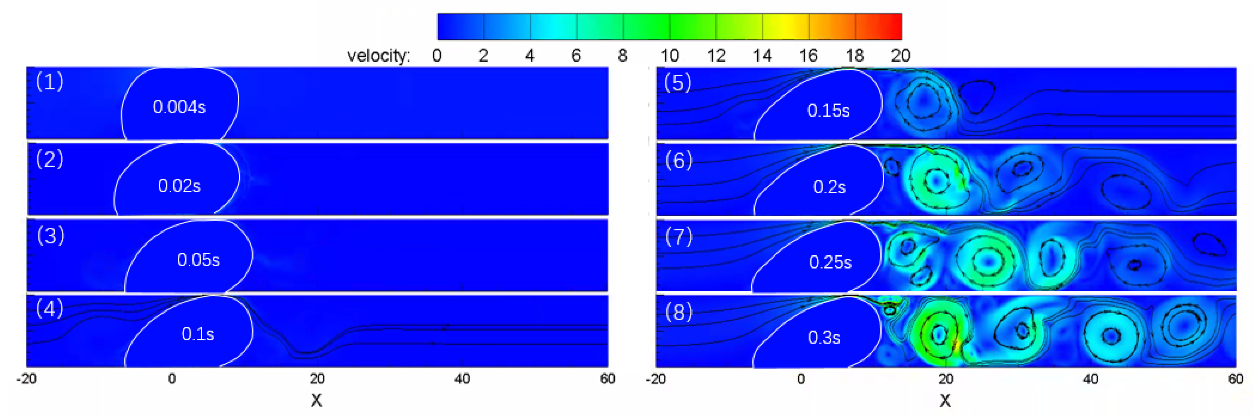
Figure 13 shows the detailed sealing strip position and flow field results. As shown in the first figure, 0.004 s is the time of the global flow peak in the first stage. At this time, the contact range between the sealing strip and the upper wall is still large, and the flow is caused by the overall movement of the sealing strip.

The second and third figures (0.02 s–0.05 s) show the second stage, that is, the process of continuous deformation when the sealing strip is still working. It can be seen that the contact position between the sealing strip and the upper edge continues to move back and the length decreases at the same time.

The fourth–seventh figures show the third stage, that is, the process in which the sealing strip begins to fail and the flow in the pipeline gradually increases. Similar to the “absolute failure” case, due to the influence of the velocity shear layer caused by the sealing structure, the fluid will inevitably form a vortex and expand continuously after passing through the slit. After reaching the restriction of the tunnel wall, the vortex size stops increasing, mainly moves downstream, then forms a new vortex behind the slit.

The eighth figure shows the results of the fourth stage. Different from the “absolute failure” case, the flow field in this case looks relatively stable, and the large-scale vortices in the flow field move downstream relatively regularly. The main reason is that, although the differential pressure setting on both sides is consistent with the absolute failure, the slit after failure is small, so the global flow rate is low. In other words, the Reynolds number of the “dynamic failure” case is low.

5. Conclusions

In this paper, a fluid–structure interaction model was established by the integration of IBM and LBM, and the deformation of the hollow sealing strip and flow field under the action of the pressure difference were simulated. The mechanical model mainly solved the problems of the superelastic characteristics of the rubber material of the sealing strip and the friction between the sealing strip and the rigid boundary. In the process of establishing the specific simulation model, a 2D calculation domain was established according to the overall dimension of an actual D-shape sealing strip and tunnel. Through the methods of wall thickness correction and corner stiffness correction, the setting of specific physical parameters was consistent with the actual situation as much as possible. The static strain of IB-LBM model was verified with the results of the FEM, which showed that this model had high accuracy.

After modeling, three typical sealing cases were simulated. The results of “non-failure” show that when there is a certain pre-compression amount and the pressure difference is relatively small, the fluid will not overcome the friction between the seal strip and the wall and the obstruction of the stiffness of the seal strip itself. The seal strip only produces small deformation and does not form flow on the two sides. The results of “absolute failure” show that compared with the case of the rigid wall, the flow field in the case of solid coupling was greatly affected by the elastic sealing strip, and the flow pulsation was large and consistent with the dithering frequency of the sealing strip. The “dynamic failure” case is similar to the combination of the above two cases, although the transition state between them is different. Importantly, as in the “absolute failure” case, after the flow field reached a relatively stable state, strong coupling between the flow field and the sealing strip was observed.

A FSI model was successfully established by IB-LBM which could effectively simulate the deformation and failure of the sealing strip under pressure differences. This model can be used for different research objectives, such as seal failure judgement, flow rate estimation, specific flow field structure study and even later can be used to study the generation of aerodynamic noise. There are many variable parameters in this model, including geometry, material properties of the sealing strip, properties of the fluid and boundary conditions such as pre-compression amount, pressure difference and loading mode. Due to space constraints, this paper did not provide comprehensive and detailed analysis results of various parameters, and more in-depth research will be carried out in the future.