Article

The Distribution of the Thermal Field in an Elliptical Electric Conductor Coated with Insulation

Faculty of Electrical Engineering, Technical University of Białystok, 45 D Wiejska St., 15-351 Białystok, Poland
*
Author to whom correspondence should be addressed.
Energies 2021, 14(21), 6880; https://doi.org/10.3390/en14216880
Submission received: 13 September 2021 / Revised: 9 October 2021 / Accepted: 17 October 2021 / Published: 20 October 2021
(This article belongs to the Section J: Thermal Management)

Abstract

:
The paper determines the stationary thermal field in an elliptical cross-section electric conductor coated with insulation. Heat is generated by the flow of alternating current (AC) through the conducting core, and then dissipated from the insulation surface via convection and radiation. The authors have developed an original method for hybrid (analytical–numerical) modeling of a field. This method has been used to solve the relevant boundary problem of Poisson’s equation. While the eigenfunctions of the Laplace operator were determined analytically, the coefficients of the eigenfunctions were calculated by iteratively solving an appropriate system of algebraic equations. The proposed method enables the analysis of systems with an elliptical geometry and a heterogeneous layered structure (e.g., air, aluminum alloy, PCV), and does not require area discretization (grid). The developed analytical–numerical (AN) method has been positively verified using finite elements (FEs). The determined thermal field is illustrated graphically. The obtained solution has a good physical interpretation.

1. Introduction

Conductors with an elliptical cross-section can be found in electrical engineering [1]. The cores of those conductors are helically stranded non-magnetic wires. For this reason, the active cross-section of conductor S1 is smaller than the surface area of the ellipse, πa1b1, where a1 and b1 are the major and the minor semi-axes of the ellipse, respectively (Figure 1). Therefore, the surface area πa1b1-S1 is filled with air. The above-described core is coated with insulation, the border of which is also an ellipse. The system presented herein can also be the model of a cylindrical conductor deformed as a result of mechanical pressure. There are also solid busbars with an elliptical cross-section [1], which are coated with heat-shrink insulation [2,3] (in this case, S1 = πa1b1). Other examples of elliptical systems include underground electric transmission cables cooled with the use of compressed gas [4], and cooled electronic systems.
Other fields of technology also use systems with elliptical cross-sections, such as compact heat exchangers, elliptical pipes carrying various fluids, geothermal systems [5], nuclear reactors, and molds for solidification in casting [4].
The analysis of the thermal field in all conductors is an important technical task [6,7,8]. Excessively high temperature (generated by the flow of current) leads to a quick decrease in the electrical and mechanical strength of the system, or even to destruction of the insulation. In the conducting part, in turn, a displacement—or, in extreme cases, delamination of the stranded wires—may occur. The thermal effects of shorting also include wire cages that may form on the conductor. Therefore, the analysis of thermal field distribution is an essential stage of checking a conductor’s design for correctness.
The literature on the subject shows that, with regard to elliptical systems, analytical, numerical, and experimental methods are used for thermal field analysis. The first group of methods includes [9]; the authors of [9] presented an analytical solution concerning the convective transfer of heat in pipes with an elliptical cross-section; they studied the flow of fluid and applied the finite series expansion method. In turn, another paper [5] investigated the temperature distribution around a cylindrical lava tube with an elliptical cross-section. In the study [5], Laplace’s equation with the Dirichlet boundary condition was solved after making appropriate simplifying assumptions; this study used the conformal mapping technique. There is also a paper [10] in which heat transfer in the laminar flow of non-Newtonian fluids in ducts with an elliptical cross-section was studied. The energy equation was solved with boundary conditions of the first and the second kind, using the generalized integral transform technique (GITT).
Numerical methods are the next group of methods of thermal field analysis in elliptical systems. An example can be found in a two-part paper [11,12] in which the flow of heat in the elliptical cross-section was modeled with the use of the finite-difference method, with boundary conditions of the third kind. Another numerical method—namely, the finite-volume method—was used in a study [13] that examined the convective heat transfer cross-flow of viscoplastic fluid in elliptical tubes. A mathematical model consisting of a mass balance equation, momentum balance equation, and energy equation in terms of temperature was analyzed in [13]. The non-Newtonian effect in the boundary layer flow over a horizontal elliptical cylinder was also examined with the use of a numerical method in another study [14], in which the boundary layer equations with boundary conditions of the first and the second kind were solved.
Experimental methods are used less often. An example can be found in a paper [4] that reports an experimental investigation into the effects of opposed lateral and vertical eccentricities on the free convective heat transfer through an elliptical annular enclosure in blunt and slender orientations. The authors of [15], in turn, described experimental and numerical analyses of natural convection that occurs in horizontal elliptical annuli.
More comprehensive literature reviews and the examples referred to above show that, for the thermal analysis of elliptical systems, analytical, numerical, and experimental methods are employed. The authors of the present paper note that (hybrid) analytical–numerical methods dedicated to elliptical systems are not used in the literature at all. This paper partially fills this gap. The essence of the method proposed by the authors consists of the analytical determination of the eigenfunctions of the Laplace operator, and the numerical determination of the coefficients of these functions.
The method proposed in this paper has a number of advantages. Compared to the numerical methods, it does not require a grid for space discretization. For this reason, the solution can be obtained at any point of the area (and not only in the grid nodes). Moreover, while the publications on analytical methods (e.g., [5,9,10]) are limited to homogeneous systems, the solutions proposed in this study enable the modelling of a layered system (i.e., one composed of different materials). The possibility of using the boundary condition of the third kind (Hankel’s) is also worth noting. To the best of the authors’ knowledge, the Hankel condition has not been used in analytical methods dedicated to elliptical systems.
As a summary of the above introduction, it can be stated that the aims of this study are as follows:
  • To determine the stationary distribution of the temperature field in an elliptical conductor coated with insulation;
  • To determine the electrical current-carrying capacity (steady-state current rating) of the above-mentioned conductor;
  • To develop the analytical–numerical method of analyzing the thermal field in a layered system with different material parameters and Hankel’s condition.

2. Physical and Mathematical Model of the System

The subject of the analysis is an elliptical conductor consisting of stranded bundles of wires coated with insulation (Figure 1). There is air between the wire bundles in the core, which is why the core was modeled as a porous body [16,17] whose thermal equivalent conductivity λ1 was determined based on [18,19]. The conductor, in turn, is insulated with an elliptical annulus made of a homogeneous PVC material with thermal conductivity λ2. The perimeters of the core η = η1 and the insulation η = η2 are confocal ellipses (Figure 1).
In a general case, the distribution of the increment in the temperature field in an immovable solid body is described by the following equation [19,20]:
d i v [ λ i g r a d   v i ( M , t ) ] c i μ i v i ( M , t ) t = g i ,
where νi(M,t) is the increment in temperature field Ti(M,t) above ambient temperature Ta at the point M and at time t in zone i:
v i ( M , t ) = T i ( M , t ) T a ,       1   for   core ,   i = 2   for   insulation ,
λi, ci, and μi are the thermal conductivity, specific heat, and mass density in zone i, respectively, while gi is the efficiency of heat sources in zone i.
The following assumptions have been made:
  • The analysis pertains to a steady state ( v i ( M , t ) = v i ( M ) v i ( M , t ) t = 0
  • Thermal conduction values for the core λ1 and insulation λ2 are constant (λi = const => d i v [ λ i g r a d ( ) ] = λ i 2 ( )
), where 2 ( ) denotes the scalar Laplace operator;
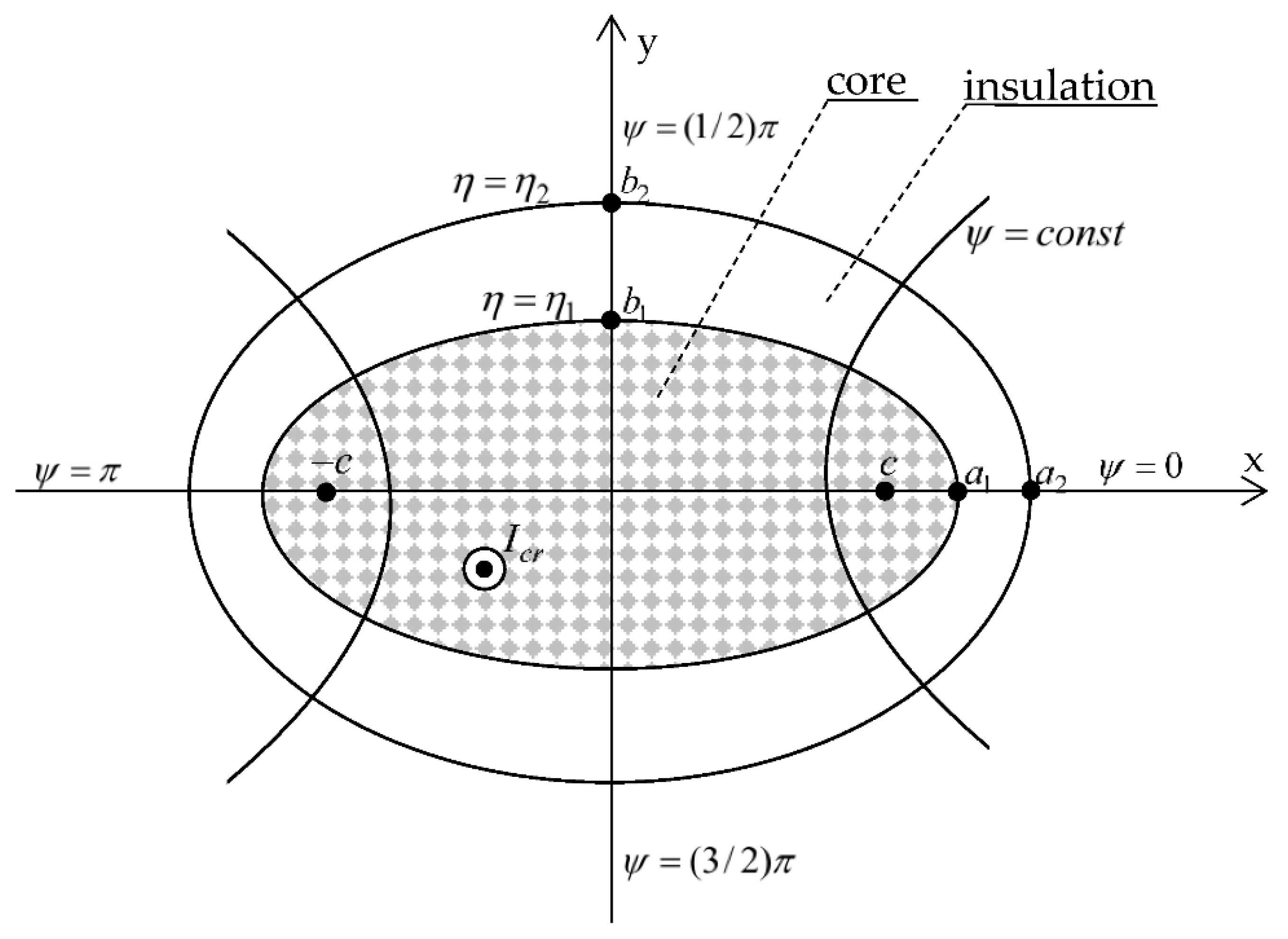
  • An elliptic–cylindrical coordinate system is used M(η,ψ,z);
  • The length of the conductor is much greater than that of the major axis of the ellipse (l >> 2a2 => νi(M) = νi(η,ψ) − case 2D).
With the abovementioned assumptions, the general heat Equation (1) can be reduced to Poisson’s equation:
1 c 2 ( cosh 2 η cos 2 ψ ) ( 2 v i ( η , ψ ) η 2 + 2 v i ( η , ψ ) ψ 2 ) = g i λ i ,   for   η i 1 η η i ,   0 ψ 2 π ,   i = 1 , 2 ,
where:
v i ( η , ψ ) = T i ( η , ψ ) T a ,
η0 = 0, and c is the abscissa of the focus.
The core is a heat source of the efficiency:
g 1 = P V ,
where P = RAC|I|2 is the thermal power generated by the flow of sinusoidal alternating current with a root-mean-square (RMS) value |I| and the mains frequency (the Joule–Lenz effect), and V = πa1b1l is the volume of the l-length core segment. The alternating-current resistance RAC can be determined by increasing the direct-current resistance RDC. For this purpose, RDC should be multiplied by skin factor kn [1] and by stranding factor ks [6]. The first factor considers the skin phenomenon, while the second factor considers the core elongation caused by the twisting of the wire bundles. Hence, the AC resistance is RAC = knksRDC = [knksρ(Tmax)l]/S1, where ρ(Tmax) is the resistivity of the core at the maximum operating temperature Tmax, and S1 is the sum of the cross-sections of the conductive bundles forming the core. By substituting the above relationships in (3a), the following was finally obtained:
g 1 = k n k s ρ ( T max ) | I | 2 S 1 π a 1 b 1 .  
Due to the low current frequency (mains frequency = 50 Hz), the displacement current in the insulation was omitted, and g2 = 0. was assumed. It was also assumed that the conductor was completely shielded from solar radiation (indoor conditions).
From Fourier’s law with respect to the normal direction ( 1 η ), and from Newton’s law of cooling [20,21], the boundary condition of the third kind (Hankel’s) results in the following equation:
1 c ( cosh 2 η cos 2 ψ ) v 2 ( η , ψ ) η | η = η 2 = α λ 2 v 2 ( η = η 2 , ψ )   for   0 ψ 2 π ,
where α is the total heat transfer coefficient considering both convection and radiation (α = αc + αr) [22]. In the denominator on the left-hand side of Equation (7), Lame’s coefficient occurs. It is most likely for this reason that the authors have not found any analytical solutions in the literature that would satisfy the Hankel condition of Equation (7) in the elliptical–cylindrical coordinates.
The equivalent zones of the core and insulation are closely adjacent to one another. Therefore, the conditions of heat flux continuity and the temperature increase on the ellipse perimeter, η = η1, are satisfied:
v 1 ( η 1 , ψ ) = v 2 ( η 1 , ψ )   for   0 ψ 2 π ,
λ 1 v 1 ( η , ψ ) η | η = η 1 = λ 2 v 2 ( η , ψ ) η | η = η 1   for   0 ψ 2 π .
The relationships resulting from the Lame coefficients of the elliptic–cylindrical system are identical on both sides of Equation (9). For this reason, the above-mentioned dependencies are omitted in the notation of Equation (9). Equations (3)–(9) given above constitute the boundary problem of the thermal field distribution, which the authors are trying to determine.

3. Solution of the Boundary Problem

In the region of the core (i = 1), the solution of the heat Equation (3) consists of the particular integral of the heterogeneous equation (i.e., the Poisson equation) and the general integral of the homogeneous equation (i.e., the Laplace equation) [23]. The particular integral for the case of the variables η,ψ of the elliptic–cylindrical system was determined based on [24]. In turn, the general integral was determined with the use of the method of separation of variables [23,24]. After the superposition of the above-mentioned integrals, the solution of Equation (3) in the core zone (i = 1) was obtained:
v 1 ( η , ψ ) = g c 2 8 λ 1 [ cosh ( 2 η ) + cos ( 2 ψ ) ] + ( C 0 + D 0 η ) ( F 0 + G 0 ψ ) +                           + n = 1 [ E n cosh ( n η ) + Γ n sinh ( n η ) ] [ K n cos ( n ψ ) + L n sin ( n ψ ) ]   for   0 η η 1 ,   0 ψ 2 π ,
where C0, D0, F0, G0, En, Γn, Kn, and Ln are either constants or coefficients.
On the other hand, in the sourceless insulation region, η1ηη2, the temperature distribution was obtained from the solution of the Laplace equation (g2 = 0)
v 2 ( η , ψ ) = ( H 0 + J 0 η ) ( W 0 + S 0 ψ ) +           + n = 1 [ P n cosh ( n η ) + Z n sinh ( n η ) ] [ X n cos ( n ψ ) + Y n sin ( n ψ ) ]   for   η 1 η η 2 ,   0 ψ 2 π .
where H0, J0, W0, S0, Pn, Zn, Xn, and Yn are either constants or coefficients.
The solutions shown above in Equations (10) and (11) must be periodic and even with respect to the coordinate ψ of the elliptic–cylindrical system. This results in the zeroing of the constants and the coefficients G0 = S0 = Ln = Yn = 0. Moreover, singular and non-physical expressions need to be eliminated. The heat flux must have a finite value at the singular point (focus). For calculating the flux, Fourier’s law q 1 = λ 1 g r a d [ T a + v 1 ( η , ψ ) ] and Equation (10) were used. It was found that in the focus of the ellipses (η = 0, ψ = 0), the flux has an infinite value. For this reason, the components containing the functions η and sinh() were discarded (D0 = Γn= 0 in (10)). After considering the above-mentioned remarks, the following solutions were obtained, where new constants and coefficients A0, An, P0, R0, Λn, and Qn were introduced:
v 1 ( η , ψ ) = g c 2 8 λ 1 [ cosh ( 2 η ) + cos ( 2 ψ ) ] + A 0 + n = 1 A n cosh ( n η ) cos ( n ψ )   for   0 η η 1 , 0 ψ 2 π ,
v 2 ( η , ψ ) = P 0 + R 0 η + n = 1 [ Λ n cosh ( n η ) + Q n sinh ( n η ) ] cos ( n ψ )   for   η 1 η η 2 , 0 ψ 2 π .
The number of constants and coefficients occurring in Equations (12) and (13) can be additionally reduced by using the conditions of temperature increment and flux continuity in Equations (8) and (9). After substituting Equations (12) and (13) into Equations (8) and (9), the following was obtained:
g c 2 8 λ 1 [ cosh ( 2 η 1 ) + cos ( 2 ψ ) ] + A 0 + n = 1 A n cosh ( n η 1 ) cos ( n ψ ) =                     = P 0 + R 0 η 1 + n = 1 [ Λ n cosh ( n η 1 ) + Q n sinh ( n η 1 ) ] cos ( n ψ ) ,
λ 1 { g c 2 4 λ 1 sinh ( 2 η 1 ) + n = 1 n A n sinh ( n η 1 ) cos ( n ψ ) } =                     = λ 2 { R 0 + n = 1 n [ Λ n sinh ( n η 1 ) + Q n cosh ( n η 1 ) ] cos ( n ψ ) } .
In Equations (14) and (15), the constants and expressions containing the cos() functions were compared (taking into consideration the special case n = 2). This led to a system of equations, the solving of which enabled a reduction in the number of constants and coefficients in Equation (13). As a result, the following was obtained:
v 2 ( η , ψ ) = A 0 g c 2 8 λ 1 cosh ( 2 η 1 ) ( η η 1 ) g c 2 4 λ 2 sinh ( 2 η 1 ) g c 2 8 λ 1 cos ( 2 ψ ) cosh [ 2 ( η η 1 ) ] +                                                                                                         + n = 1 A n [ f ( n ) cosh ( n η ) + g ( n ) sinh ( n η ) ] cos ( n ψ )
where:
f ( n ) = cosh 2 ( n η 1 ) λ 1 λ 2 sinh 2 ( n η 1 ) ,
g ( n ) = λ 1 λ 2 2 λ 2 sinh ( 2 n η 1 ) .
In Equations (12) and (16), unknown coefficients A0 and An remained. They were determined using the Hankel boundary condition in Equation (7) (of the third kind). For this purpose, the sum of the series (Equation (16)) was limited to a finite number of terms N and substituted into Equation (7). This resulted in the following:
1 c cosh 2 ( η 2 ) cos 2 ( ψ ) ( g c 2 4 λ 2 sinh ( 2 η 1 ) g c 2 4 λ 1 cos ( 2 ψ ) sinh [ 2 ( η 2 η 1 ) ] + + n = 1 N n A n { f ( n ) sinh ( n η 2 ) + g ( n ) cosh ( n η 2 ) } cos ( n ψ ) ) = = - α λ 2 ( A 0 g c 2 8 λ 1 cosh ( 2 η 1 ) ( η 2 η 1 ) g c 2 4 λ 2 sinh ( 2 η 1 ) g c 2 8 λ 1 cos ( 2 ψ ) cosh [ 2 ( η 2 η 1 ) ] + + n = 1 N A n { f ( n ) cosh ( n η 2 ) + g ( n ) sinh ( n η 2 ) } cos ( n ψ ) ) .
Equation (19) was multiplied by {cos()} and then integrated by sides with respect to the angular coordinate {ψ} in the range <0,2π>. In this way, Equation (20) was obtained for m = 1,2…N. The next equation (Equation (21)) was obtained by integrating the two sides of the relationship in Equation (19) with respect to the angular coordinate {ψ} in the range <0,2π>. As a result of the operations described above, a system of N + 1 equations with respect to unknowns A0…An was obtained:
{ (20) n = 1 N A n I 1 ( m , n ) = I 2 ( m )   for   m = 1 , 2 ... N , (21) n = 1 N A n I 3 ( n ) + A 0 2 π α λ 2 = I 4
where:
I 1 ( m , n ) = r ( n ) h ( m , n ) ,   for m n ,
I 1 ( m = n ) = r ( m ) h ( m = n ) + π α λ 2 [ f ( m ) cosh ( m η 2 ) + g ( m ) sinh ( m η 2 ) ] ,
I 2 ( m ) = g c sinh ( 2 η 1 ) 4 λ 2 h ( m , n = 0 ) + g c sinh [ 2 ( η 2 η 1 ) ] 4 λ 1 h ( m , n = 2 )   for     m 2 ,
I 2 ( m = 2 ) = g c sinh ( 2 η 1 ) 4 λ 2 h ( m = 2 , n = 0 ) + g c sinh [ 2 ( η 2 η 1 ) ] 4 λ 1 h ( m = n = 2 ) + + π g c 2 α cosh [ 2 ( η 2 η 1 ) ] 8 λ 1 λ 2 ,
I 3 ( n ) = r ( n ) h ( m = 0 , n ) ,
I 4 = g c sinh ( 2 η 1 ) 4 λ 2 h ( m = n = 0 ) + g c sinh [ 2 ( η 2 η 1 ) ] 4 λ 1 h ( m = 2 , n = 0 ) +                             + π g c 2 α cosh ( 2 η 1 ) 4 λ 1 λ 2 + π g c 2 α ( η 2 η 1 ) 2 λ 2 2 sinh ( 2 η 1 ) ,
h ( m , n ) = 0 2 π cos ( m ψ ) cos ( n ψ ) d ψ cosh 2 ( η 2 ) cos 2 ( ψ )
r ( n ) = n c [ f ( n ) sinh ( n η 2 ) + g ( n ) cosh ( n η 2 ) ] ,
where the discrete functions f(n) and g(n) were defined using Equations (17) and (18).
Some fragments of the above relationships can be transformed into complete elliptic integrals of the first kind [25]. However, it is much easier to calculate h() in Equations (22)–(28) using an arbitrary numerical integration method [26]. After determining the integrals in Equations (22)–(28), the system of Equations (20) and (21) was iteratively solved [26] to compute the coefficients An and A0. Finally, field distributions were obtained after taking into consideration the definition of the increment in Equation (4) by adding ambient temperature Ta to the right-hand sides of Equations (12) and (16).

4. Calculation Example

As a calculation example, an elliptic conductor consisting of stranded aluminum alloy bundles with an active cross-section S1 = 270 mm2 was taken into consideration. The system was coated with PVC insulation. The following data were assumed:
b1 = 0.0069098 m, a1 = 2b1, a2 = 0.0165837 m, b2 = 0.0114796 m, λ1 = 180 W/(mK), λ2 = 0.17 W/(mK), α = 14.9 W/(m2K), Tmax = 70 °C, Ta = 25 °C, ks = 1.02, kn = 1.02, ρ(70 °C) = 3.39592·10−8 Ωm.
Based on the above dataset, the following secondary parameters of the elliptical system were also determined: the coordinate of the ellipse focus c = a 1 2 b 1 2 , and the equations of the perimeter of the core η = η1 = arsinh(b1/c) and the insulation η = η2 = arsinh(b2/c) [24]. The space between the wire bundles was additionally filled with air. Therefore, the equivalent thermal conductivity λ1 of the porous body [18] was smaller than that of the solid aluminum alloy (λ1 < 200 W/(mK)).
The software for the presented method (Section 3) was developed in the Mathematica 11.1 environment [26], which is widely used in scientific calculations. The users have no access to the source code. Below, the basic functional blocks of the program are listed, and the percentage shares of the time of their execution are given:
  • Numerical computation of the integrals in Equations (22)–(28) and the iterative solution of the system of Equations (20) and (21) with a dense matrix of coefficients: 97%;
  • Summation of Equations (12) and (16), conversion of the elliptical coordinates into the Cartesian coordinates, and the visualization of the results: 3%.
In the case of using a PC with an I7-5820K processor with a clock frequency of 3.3 GHz, furnished with 16 GB RAM and an SSD 500 GB hard drive, the total computation time is 280 s:100%.
While computing field distributions, the infinite series in Equations (12) and (16) showed a strong convergence. When adding more than 12 terms, the results of computation at each point of the region varied at the 6th decimal place. For this reason, the summing of the series was limited to N = 12.
One of the most important conductor parameters is the steady-state current rating Icr. This is limited by the highest value of temperature Tmax to which the conductor insulation may heat up (with no risk of being damaged) under sustained current load conditions. Insulation is the most exposed to overheating at contact with the core at the point situated the closest to the heat source center. This location is also implied by the greatest insulation thickness b2b1 above this point (Figure 1). The relatively large b2b1 value hampers the heat outflow from the core to the environment. The lower and upper co-vertices of the core surface (Figure 1) meet the conditions described above. These are the hottest points of the perimeter η = η1. Therefore, in order to find the steady-state current rating, the following equation should be solved:
T 1 ( η = η 1 , ψ = π 2 , I c r ) = T max .
Equation (31) was solved iteratively in the Mathematica 11.1 program [26]. For the data from the set in (30), the result Icr = 574.5 A was obtained. Then, for this current, the thermal field in the elliptic conductor was determined. For more convenient observation, the selected distributions are presented in the Cartesian coordinate system x = c∙coshη∙cosψ, y = c∙sinhη∙sinψ. Figure 2 and Figure 3 illustrate temperature changes on the major axis (y = 0, Figure 2) and on the minor axis (x = 0, Figure 3), respectively. Figure 4, in turn, shows the two-dimensional distribution of the temperature field on the conductor cross-section with the current provided above.

5. Numerical Verification of the Solution

Equations (12) and (16) were replaced with the sum of the first 12 terms. In this section, it was verified whether such an approximation leads to the correct results. It was also necessary to eliminate possible errors of a different type. For this reason, the boundary problem of Equations (3)–(9) was solved again using the finite-element (FE) method [27,28]. This method is the basis of the professional COMSOL Multiphysics [29] program that was used for the numerical analysis. It should be emphasized that the FE and AN methods (Section 3) are completely different.
The relative differences in temperature increments were calculated from the following formula:
δ T i = v i ( x , y ) v i ( F E ) ( x , y ) v i ( x , y ) 100 % for   i = 1 , 2 ,
where v i ( x , y ) is the temperature increase distribution obtained using the AN (analytical–numerical) method in the i-th zone, while v i ( F E ) ( x , y ) represents th temperature increase distribution calculated using the FE method in the i-th zone. Figure 5 and Figure 6 illustrate the relationship in Equation (32) on the major axis (y = 0, Figure 5) and on the minor axis (x = 0, Figure 6) of the ellipses, respectively. At points not located on the axes (x ≠ 0 and y ≠ 0), the relative differences of Equation (32) are similar to those shown in Figure 5 and Figure 6.

6. Final Remarks

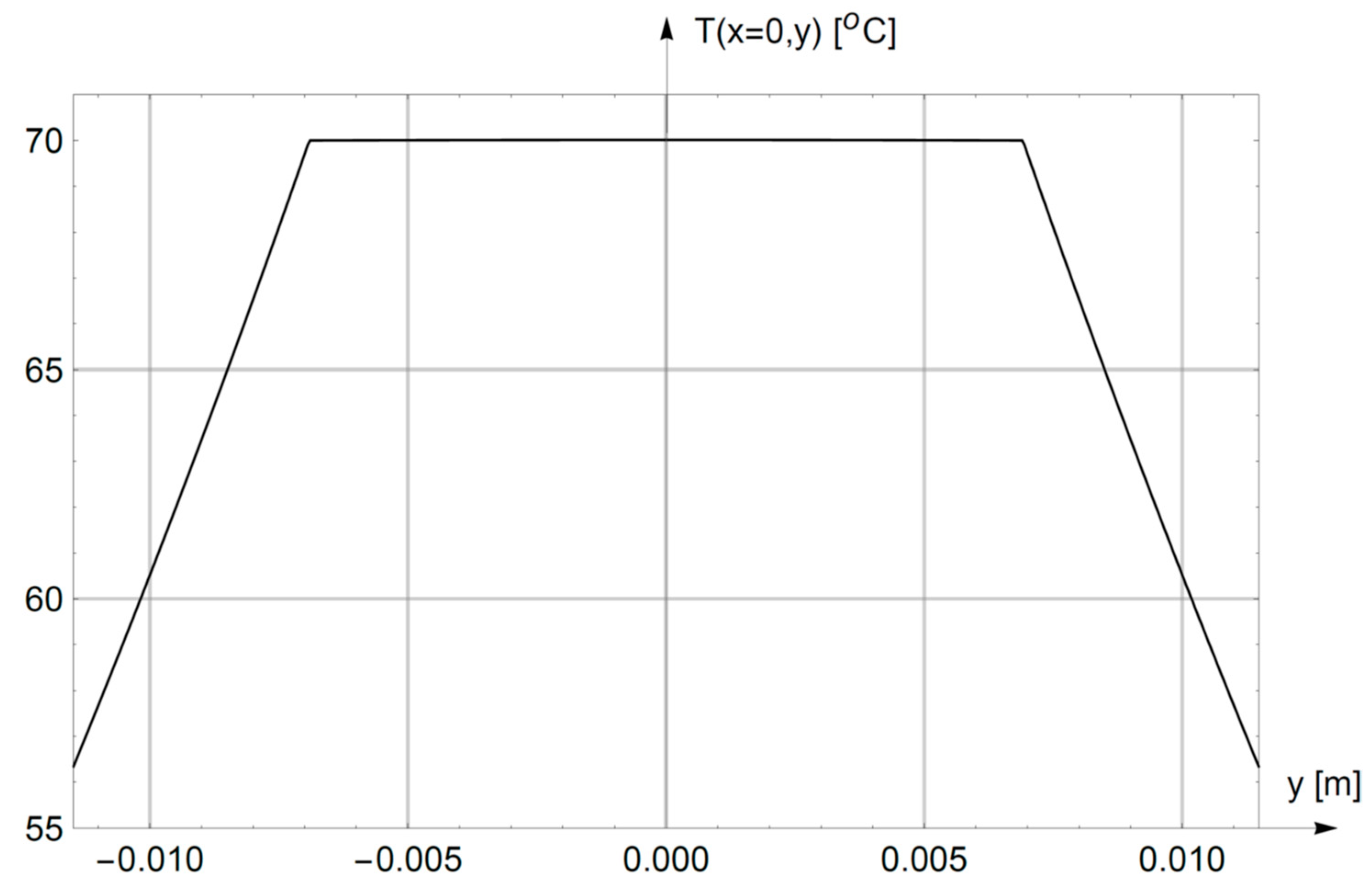
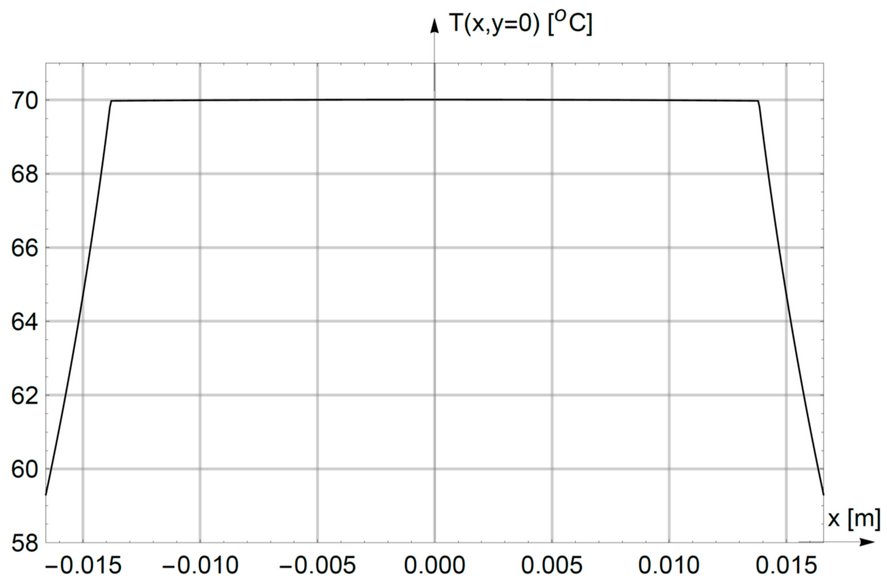
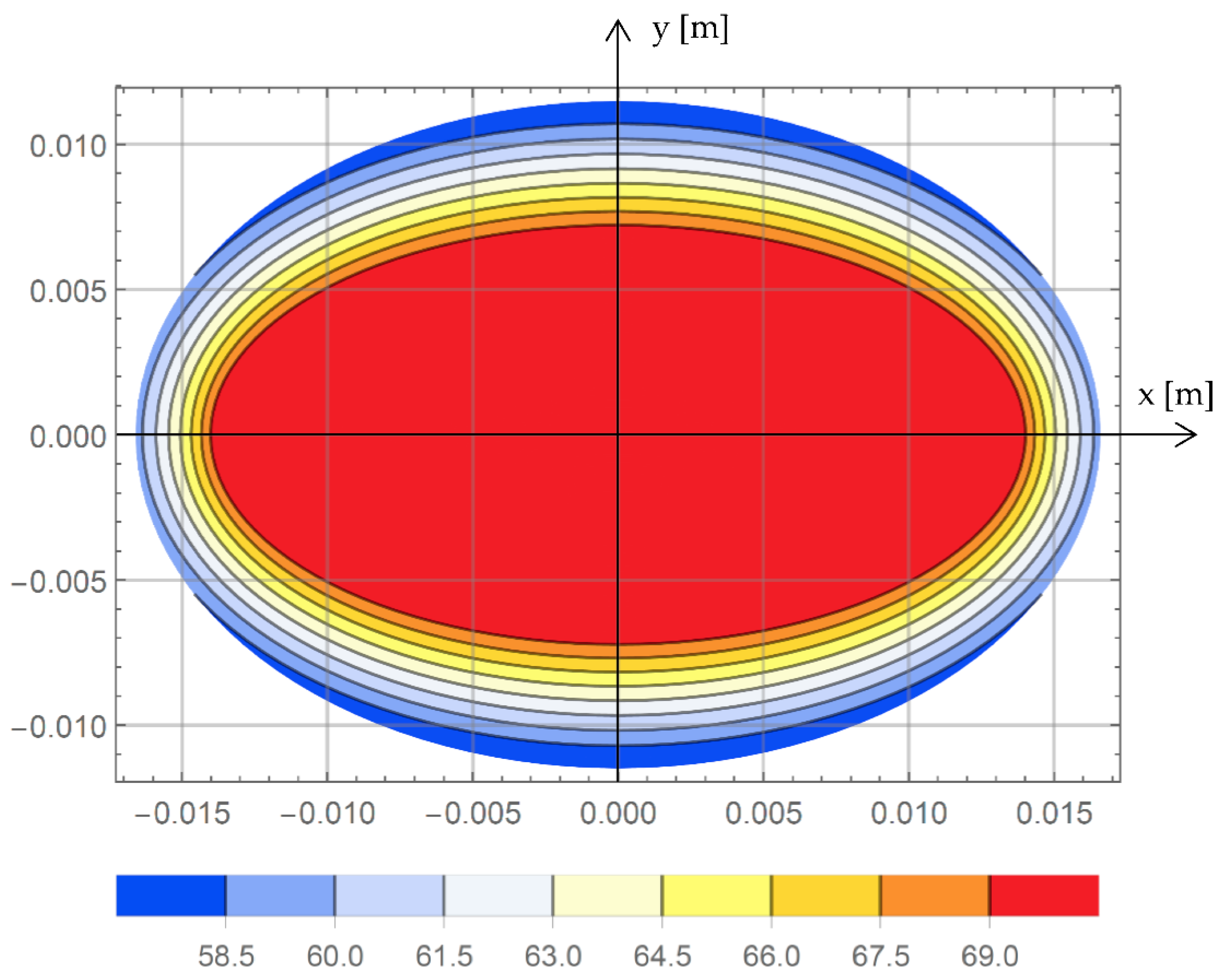
  • The thermal field in the core (0 ≤ η ≤ η1) is almost uniform, as can be seen in Figure 2, Figure 3 and Figure 4. The maximum temperature drop in the core is merely T1(η = 0, ψ = π/2) − T1(η = η1, ψ = 0) = 0.034 °C. The physical cause of the above-mentioned phenomenon is the very large equivalent thermal conductivity λ1 of the porous system (aluminum alloy-air) with a packing of (S1/πa1b1) ≈ 0.9;
  • Distinct temperature drops occur in PVC insulation (η1 ≤ η ≤ η2), as can be seen in Figure 2, Figure 3 and Figure 4. This temperature drop increases with the thickness of the insulation {(b2b1) 4.57 mm > (a2a1) 2.76 mm} = >{[T2(η = η1, ψ = π/2) − T2(η = η2, ψ = π/2)] = 13.66 °C >> [T2(η = η1, ψ = 0) − T2(η = η2, ψ = 0)] = 10.676 °C}—see Figure 1. The above results from the fact that the thermal resistance of the insulation increases with an increase in its thickness, as well as from Ohm’s thermal law [22]. The temperature drops are nearly linear (Figure 2 and Figure 3);
  • The perimeters of the core (η = η1) and the insulation (η = η2) are not isotherms. For η = η1, the temperature changes from T1(η1,ψ = 0) = 69.976 °C to T1(η1,ψ = π/2) = 70 °C, while for η = η2 it changes from T2(η2,ψ = π/2) = 56.34 °C to T2(η2,ψ = 0) = 59.3 °C. The above is due to a change in the distance of points on the perimeters η = η1 and η = η2 from the center of the heat source (η = 0, ψ = π/2). Another cause is the variation in insulation thickness with the coordinate ψ;
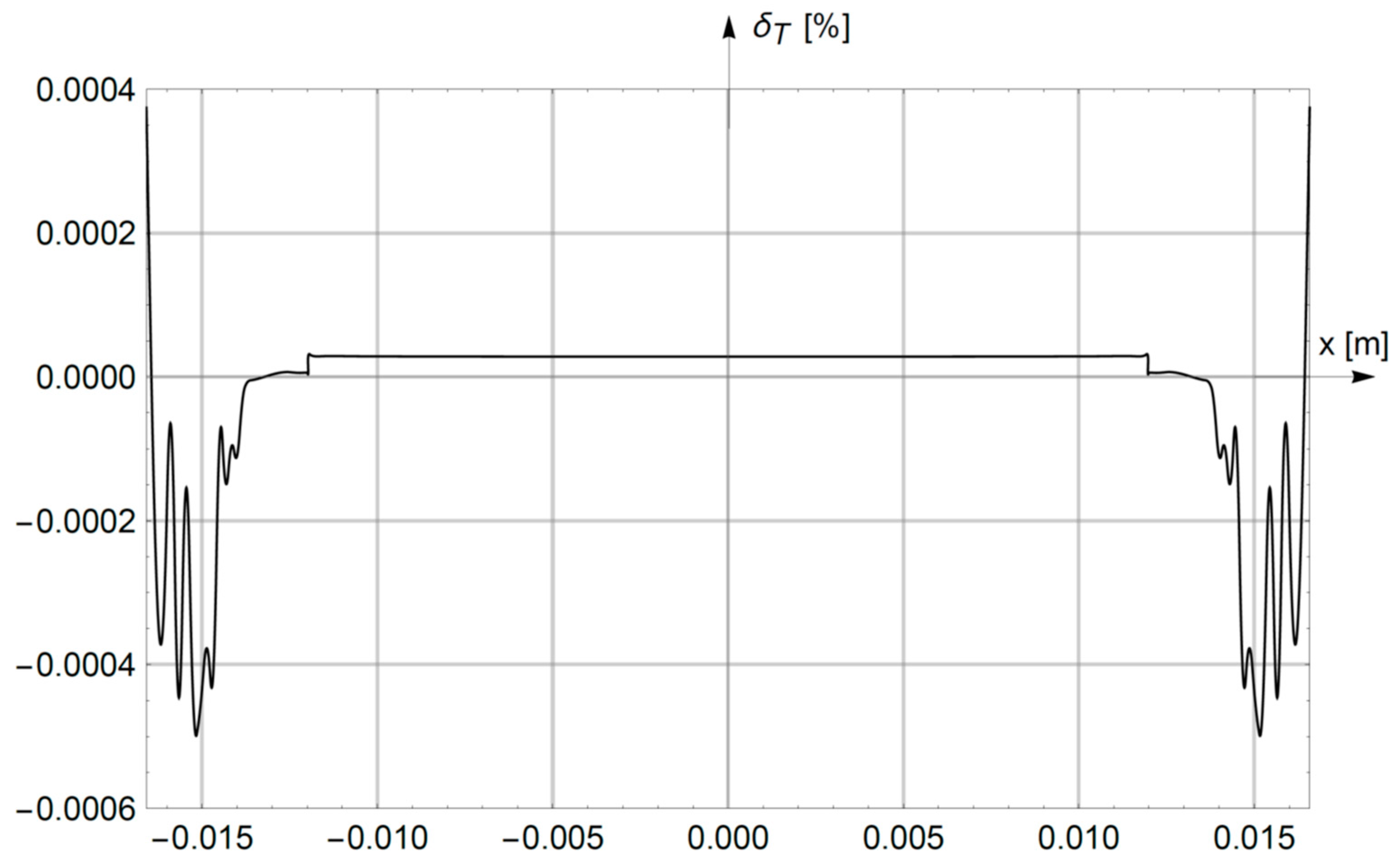
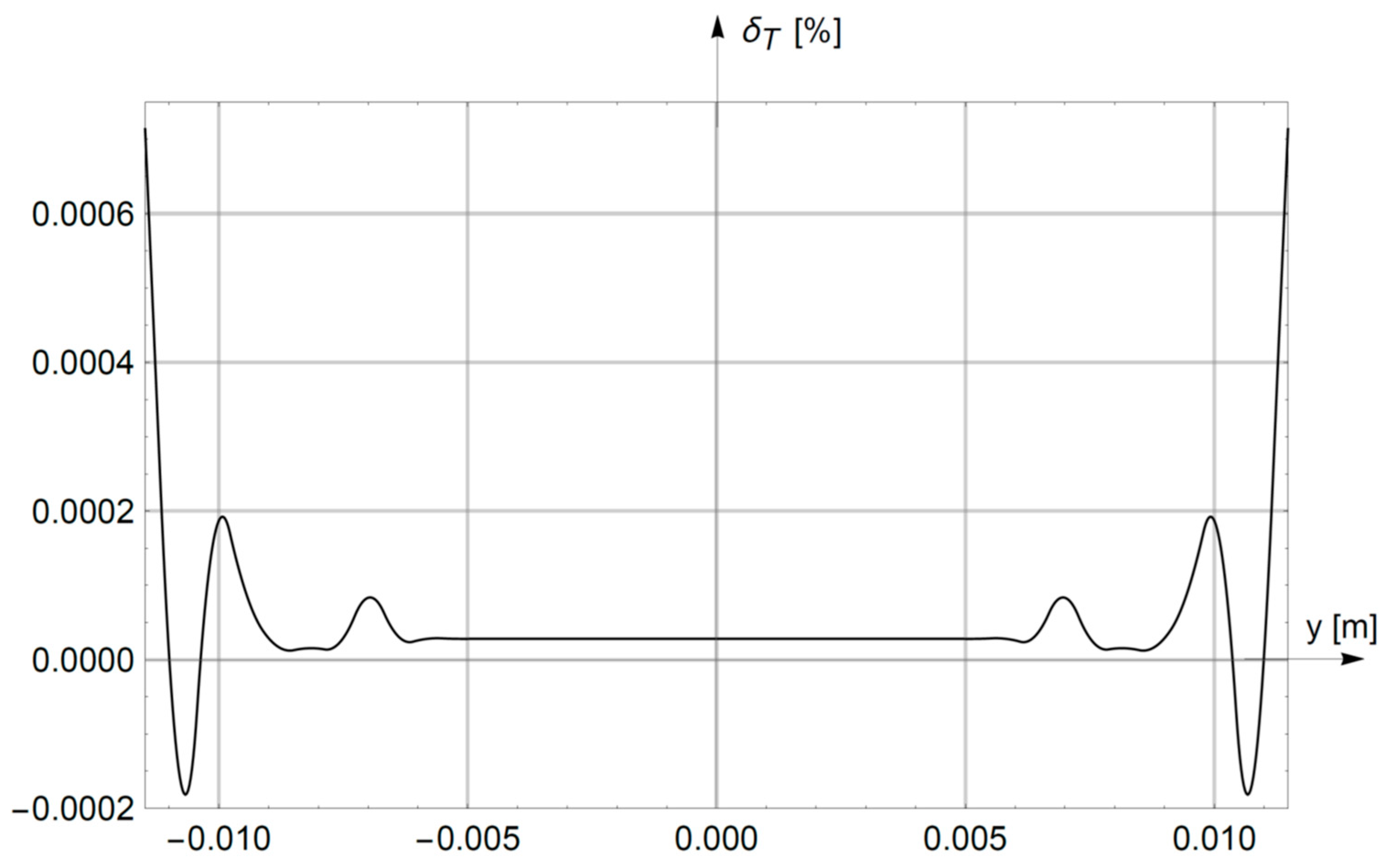
  • The relative differences between the temperature distributions in Equation (32) (calculated using the analytical–numerical (AN) method and the finite-element (FE) method) are very small. On the major axis y = 0, the module (32) is smaller than 0.0005% (Figure 5), while on the minor axis x = 0, T2| < 0.00075% is true (Figure 6). The smallest differences in Equation (32) are found in the region of uniform field (i.e., in the core). Slightly greater deviations δT2 are observed in the area of temperature drop (i.e., in the insulation); this results from the inequality λ1 >> λ2. Due to the small values of relative differences in Equation (32), the developed AN method leads to practically the same results as the commonly used numerical FE method.

7. Conclusions

An analytical–numerical (AN) method was developed in this paper for determining the stationary temperature field in an elliptical conductor coated with insulation (Figure 1). The eigenfunctions of the Laplace operator Equations (12) and (16) were determined analytically by the superposition of the general and particular integrals of the Poisson Equation (3) [23], and by the variable-separation method [23]. On the other hand, the coefficients of the eigenfunctions were determined by iteratively solving the system of Equation (20) and (21) (e.g., using the Krylov method [26]) after previously calculating the integrals in Equation (22)–(28) (i.e., using the trapezoid method). The presented AN method enables the modeling of heterogeneous layered systems and boundary problems of the third kind (Hankel Equation (7)) in elliptic geometries. This represents distinct progress compared to analytical methods. In addition, the AN solution can be obtained in the entire area (and not only at discrete points, as in the majority of numerical methods). The developed analytical–numerical method was positively verified using the finite-element method.

Author Contributions

The authors equally contributed to the preparation of each excerpt of the paper: 50%, J.G.; 50%, M.Z. All authors have read and agreed to the published version of the manuscript.

Funding

The paper was prepared at Bialystok University of Technology within the framework of the W/WE-IA/2/2020 project funded by Ministry of Education and Science, Poland.

Institutional Review Board Statement

Not applicable.

Informed Consent Statement

Not applicable.

Data Availability Statement

Not applicable.

Conflicts of Interest

The authors declare no conflict of interest.

List of Symbols

A0Constant in Equation (12)
AnCoefficient in Equation (12)
a1Major semi-axis of the ellipse η = η1 (core surface)—Figure 1
a2Major semi-axis of the ellipse η = η2 (insulation surface)—Figure 1
b1Minor semi-axis of the ellipse η = η1 (core surface)—Figure 1
b2Minor semi-axis of the ellipse η = η2 (insulation surface)—Figure 1
C0, D0, F0, G0Constants in Equation (10)
cAbscissa of the focus
ciSpecific heat (i = 1 for core, i = 2 for insulation)
En, Γn, Kn, LnCoefficients in Equation (10)
f(n) Discrete function defined by Equation (17)
giEfficiency of heat sources (i = 1 for core, i = 2 for insulation)
g(n) Discrete function defined by Equation (18)
H0, J0, W0, S0Constants in Equation (11)
h(m,n)Integral defined by Equation (28)
I1(m,n), I2(m), I3(n), I4Integrals defined by Equations (22)–(27)
|I|Root-mean square (RMS) current
IcrSteady-state current rating
knSkin factor
ksStranding factor
lLength of the conductor segment
NNumber of summed terms of Equations (12) and (16)
nSummation index
PThermal power
P0, R0Constants in Equation (13)
Pn,Zn,Xn,YnCoefficients in Equation (11)
Qn, ΛnCoefficients in Equation (13)
q 1 Heat flux vector
RACAlternating-current resistance
RDCDirect-current resistance
r(n)Discrete function defined by Equation (29)
S1Sum of the cross-sections of the conductive bundles (active cross-section)
TaAmbient temperature
TmaxMaximum operating temperature
VVolume of the l-length core segment
Ti(..,..)Temperature distributions (i = 1 for core, i = 2 for insulation)
αTotal heat transfer coefficient
αcConvective heat transfer coefficient
αrRadiation heat transfer coefficient
δTiRelative differences in temperature increments defined by Equation (32)
η1Perimeter of the core (η = η1)
η2Perimeter of the insulation (η = η2)
(η,ψ)Coordinates of an elliptical–cylindrical system
λiThermal conductivity (i = 1 for core, i = 2 for insulation)
μiMass density (i = 1 for core, i = 2 for insulations)
νi(..,..) Temperature increase obtained using the AN method (i = 1 for core, i = 2 for insulation)
v i ( F E ) ( . , . ) Temperature increase calculated using the FE method (i = 1 for core, i = 2 for insulation)
ρ(Tmax)Resistivity of the core at the maximum operating temperature
1 η Unit vector normal to the surface η = const
2 ( ) Scalar Laplace operator

References

  1. Morgan, V.T. The current distribution, resistance and internal inductance of linear power system conductors—A review of explicit equations. IEEE Trans. Power Deliv. 2013, 38, 1252–1262. [Google Scholar] [CrossRef]
  2. 3M Electrical Product Division. 3MTM Heat Shrinkable Tubing for Bus Bar BBI-A Series 5–35 kV; 3M Inc.: Austin, Texas, USA, 2013. [Google Scholar]
  3. ABB Catalogue Heat Shrink. Heatshrink Solutions Insulate, Identify and Protect Your Wires and Cables; ABB Inc.: London, UK, 2016. [Google Scholar]
  4. Eid, E.I.; Abdel-Halim, M.; Easa, A.S. Effect of opposed eccentricity on free convective heat transfer trough elliptical annulus enclosures in blunt and slender orientations. Heat Mass Transf. 2015, 51, 239–250. [Google Scholar] [CrossRef]
  5. Dragoni, M.; Tallarico, A. Temperature field and heat flow around an elliptical lava tube. J. Volcanol. Geotherm. Res. 2008, 169, 145–153. [Google Scholar] [CrossRef]
  6. Anders, G.J. Rating of Electric Power Cables: Ampacity Computations for Transmission, Distribution and Industrial Application; McGraw-Hill Professional: New York, NY, USA, 1997. [Google Scholar]
  7. IEEE Std. 738-2012. IEEE Standard for Calculating the Current-Temperature Relationship of Bare Overhead Conductors; IEEE Standard Association: Piscataway Township, NJ, USA, 2013. [Google Scholar]
  8. CIGRE Working Group B2.42. Guide for Thermal Rating Calculations of Overhead Lines, Technical Brochure 601; CIGRE: Paris, France, 2014. [Google Scholar]
  9. Shahmardan, M.M.; Norouzi, M.; Sedaghat, M.H. An exact analytical solution for convective heat transfer in elliptical pipes. AUT J. Mech. Eng. 2017, 1, 131–138. [Google Scholar]
  10. Maia, C.R.M.; Aperecido, J.B.; Milanez, L. F Heat transfer in laminar flow of non-Newtonian fluids in ducts of elliptical section. Int. J. Therm. Sci. 2006, 45, 1066–1072. [Google Scholar] [CrossRef]
  11. Erdoğdu, F.; Bulaban, M.O.; Chau, K.V. Modeling of heat conduction in elliptical cross section: I. Development and testing of the model. J. Food Eng. 1998, 38, 223–239. [Google Scholar] [CrossRef]
  12. Erdoğdu, F.; Bulaban, M.O.; Chau, K.V. Modeling of heat conduction in elliptical cross section: II. Adaptation to thermal processing of shrimp. J. Food Eng. 1998, 38, 241–258. [Google Scholar] [CrossRef]
  13. Hermany, L.; Lorenzini, G.; Klein, R.J.; dos Santos, E.D.; Isoldi, L.A.; Rocha, L.A.O. Constructal design applied to elliptic tubes in convective heat transfer cross-flow of viscoplastic fluids. Int. J. Heat Mass Transf. 2018, 116, 1054–1063. [Google Scholar] [CrossRef]
  14. Nag, P.; Molla, M.M.; Hossain, M.A. Non-newtonian effect on natural convection flow over cylinder of elliptic cross section. Appl. Math. Mech. 2020, 41, 361–382. [Google Scholar] [CrossRef]
  15. Sakr, R.Y.; Berbish, N.S.; Abd-Alziz, A.A.; Hanafi, A.S. Experimental and numerical investigation of natural convection heat transfer in horizontal elliptic annuli. J. Appl. Sci. Res. 2008, 4, 138–155. [Google Scholar] [CrossRef]
  16. Hoseinzadeh, S.; Sohani, A.; Ashrafi, T.G. An artificial intelligence-based predition way to describe flowing a Newtonian liquid/gas on a permeable flat surface. J. Therm. Anal. Calorim. 2021, 1, 1–7. [Google Scholar]
  17. Hoseinzadeh, S.; Sohani, A.; Shahverdian, M.H.; Shirkhani, A.; Heyns, S. Acquiring an analytical solution and performing a comparative sensitivity analysis for flowing Maxwell upper-convected fluid on a horizontal surface. Therm. Sci. Eng. Prog. 2021, 23, 100901. [Google Scholar] [CrossRef]
  18. Nield, D.A.; Bejan, A. Convection in Porous Media; Springer-Verlag: New York, NY, USA, 2013. [Google Scholar]
  19. Latif, M.J. Heat Conduction; Springer-Verlag: Haidelberg, Germany, 2009. [Google Scholar]
  20. Hahn, D.W.; Ozisik, M.N. Heat Conduction; John Wiley & Sons: Hoboken, NJ, USA, 2012. [Google Scholar]
  21. Taler, J. Solving Direct and Inverse Heat Conduction Problems; Springer-Verlag: Berlin, Germay, 2016. [Google Scholar]
  22. Bergman, T.L.; Lavine, A.S.; Incropera, F.P.; Dewitt, D.P. Fundamentals of Heat and Mass Transfer; John Wiley and Sons: Hoboken, NJ, USA, 2011. [Google Scholar]
  23. Evans, L.C. Partial Differential Equations; American Mathematical Society: Providence, RI, USA, 2010. [Google Scholar]
  24. Moon, P.; Spencer, D.E. Field Theory Handbook; Springer-Verlag: Berlin, Germany, 1988. [Google Scholar]
  25. Abramowitz, A.; Stegun, I.A. Handbook of Mathematical Functions with Formulas, Graphs, and Mathematical Tables; Dover Publications, Inc.: New York, NY, USA, 1972. [Google Scholar]
  26. Wolfram Research Inc. Mathematica; Wolfram Research Inc.: Champaign, IL, USA, 2020. [Google Scholar]
  27. Nithiarasu, P.; Lewis, R.W.; Seetharamu, K.N. Fundamentals of the Finite Element Method for Heat and Mass Transfer; John Wiley and Sons: Chichester, UK, 2016. [Google Scholar]
  28. Brener, S.; Scott, R.L. The Mathematical Theory of Finite Element Method; Springer: Berlin, Germany, 2008. [Google Scholar]
  29. COMSOL Multiphysics. Documentation for COMSOL; Release 4.3; Comsol Inc.: Stockholm, Sweden, 2013. [Google Scholar]
Figure 1. The cross-section of the elliptical conductor in the elliptic and Cartesian coordinate systems.
Energies 14 06880 g001
Figure 2. Temperature distribution on the major axis (y = 0) of the elliptic conductor under current load Icr = 574.5 A.
Energies 14 06880 g002
Figure 3. Temperature distribution on the minor axis (x = 0) of the elliptical conductor under current load Icr = 574.5 A.
Energies 14 06880 g003
Figure 4. Thermal field distribution in the cross-section of the elliptical conductor under current load Icr = 574.5 A.
Energies 14 06880 g004
Figure 5. Relative differences (Equation (32)) between the results of the analytical–numerical method and the finite-element method for y = 0 (on the major axis of the ellipse).
Energies 14 06880 g005
Figure 6. Relative differences (Equation (32)) between the results of the analytical–numerical method and the finite-element method for x = 0 (on the minor axis of the ellipse).
Energies 14 06880 g006
Publisher’s Note: MDPI stays neutral with regard to jurisdictional claims in published maps and institutional affiliations.

