Influence of Selected Non-Ideal Aspects on Active and Reactive Power MRAS for Stator and Rotor Resistance Estimation

Abstract

Mathematical models of induction motor (IM) used in direct field-oriented control (DFOC) strategies are characterized by parametrization resulting from the IM equivalent circuit and model-type selection. The parameter inaccuracy causes DFOC detuning, which deteriorates the drive performance. Therefore, many methods for parameter adaptation were developed in the literature. One class of algorithms, popular due to their simplicity, includes estimators based on the model reference adaptive system (MRAS). Their main disadvantage is the dependence on other machines’ parameters. However, although typically not considered in the respective literature, there are other aspects that impair the performance of the MRAS estimators. These include, but are not limited to, the nonlinear phenomenon of iron losses, the effect of necessary discretization of the algorithms and selection of the sampling time, and the influence of the supply inverter nonlinear behavior. Therefore, this paper aims to study the effect of the above-mentioned negative aspects on the performance of selected MRAS estimators: active and reactive power MRAS for the stator and rotor resistance estimation. Furthermore, improved reduced-order models and MRAS estimators that consider the iron loss phenomenon are also presented to examine the iron loss influence. Another merit of this paper is that it shows clearly and in one place how DFOC, with the included effect of iron losses and inverter nonlinearities, can be modeled using simulation tools. The modeling of the IM and DFOC takes place in MATLAB/Simulink environment.

1. Introduction

Mathematical models of the induction motor (IM) are needed for two purposes: the modeling of the machine itself and for the real-time high-performance control strategies, among which we can include field-oriented control (FOC), direct torque control (DTC), and model predictive control (MPC) [1]. The set of the parameters utilized by the mathematical models is defined by the IM equivalent circuit selection and model type [2,3,4]. The key parameters in the traditional T-equivalent circuit are the stator and rotor resistances, leakage inductances, and magnetizing inductance. Unfortunately, these parameters are not constant during the drive operation since they are affected mainly by the temperature rise and magnetic flux saturation [5]. For instance, the nonlinear magnetizing characteristics can be respected within the control algorithm using offline-measured data. However, the compensation of the resistances must be handled online since it depends on the machine’s loading.

So far, numerous online identification methods of IM parameters have been proposed in the literature. These include model-based methods [6], recursive least-square algorithms (RLS) [7,8,9], model reference adaptive systems (MRAS) [10,11,12,13,14,15,16], signal injection (SI) techniques [17,18,19], state observers (SO) [20,21,22], and artificial intelligence (ANN) [23,24,25] methods. Typically, the greater the estimation accuracy and insensitivity to other machine parameters, the greater the algorithm complexity, which puts demands on hardware computational power and the experience of the implementation engineer. Therefore, due to the ease of implementation, MRAS-based estimators are quite popular for IM speed or parameter estimation.

The basic MRAS principle is that two mathematical models are evaluated parallelly: the so-called reference and adaptive. The reference model does not depend on the estimated quantity. On the contrary, the adaptive model utilizes the estimated quantity directly or indirectly. An adaptation mechanism (usually a simple PI controller) estimates the desired variable by driving the difference between the reference and adaptive model to zero. For the MRAS design, the Lyapunov theory or hyperstability theory can be utilized [11].

Numerous MRAS estimators based on various quantities have been proposed in the literature so far. These include MRAS based on: reactive power [10,11,12,13,14], rotor flux [26,27,28], active power [29,30], PY fictitious quantity [31], X fictitious quantity [32], $q$-axis rotor flux [33], $d$-axis air-gaip flux [34], $d$-axis stator voltage [35], or electromagnetic torque [14]. The major drawback of the MRAS schemes is that they inherently suppose that the error between the reference and adaptive model is caused by the estimated parameter only. The papers that focus on MRAS techniques usually strive to analyze the estimation process in terms of the stability [11,12,13] and sensitivity to the machine parameters [36,37] or speed [30,38,39]. However, other issues affecting the parameter estimation that are usually not acknowledged or examined in the respective papers include:

• Effect of solver and sampling time selection. MRAS design is, in most cases, carried out in the continuous-time domain. However, the actual control algorithms are implemented on a discrete system: either a digital signal processor (DSP) or field-programmable gate array (FPGA). Only a few papers consider the effect of discretization [40,41]. However, they are focused on a specific MRAS for speed estimation.
• Effect of voltage-source inverter (VSI) nonlinearity. Most of the MRAS algorithms utilize directly or indirectly the stator voltage vector. As the real-time voltage measurement is hardware demanding and requires properly designed filters, the reference voltage (i.e., the input to the modulator) is usually utilized instead of the direct measurement. However, the fundamental output voltage of the commonly used IGBT inverters is distorted, mainly due to the inserted deadtime and finite semiconductor switching.
• Effect of iron losses. Iron losses are a phenomenon that undoubtedly affects the IM flux, torque, speed, and parameter estimation [42,43,44]. However, most of the proposed MRAS estimators are based on IM equivalent circuits that do not consider iron losses.

This paper aims to examine and quantify the influence of the issues mentioned above on the performance of MRAS-type IM parameter estimators. The most popular reactive power MRAS (Q-MRAS) for the rotor resistance estimation and active power MRAS (P-MRAS) for the stator resistance estimation are selected as the candidates for the investigation. The presented results are based on simulations of the direct FOC (DFOC) of a 3.6 kW IM drive in the MATLAB/Simulink because, in a real drive, it is not possible to efficiently study the decoupled effects of various phenomena acting on the system. For machine modeling, the traditional T-equivalent circuit is utilized. The circuit is augmented with the fictitious iron loss resistance placed in parallel with the magnetizing branch to study the effect of iron losses.

This paper is organized as follows: Section 2 shows full-order state-space models of IM with and without the included effect of iron losses that are used to model the machine itself. Section 3 then presents improved reduced-order models with the included effect of iron losses used in the DFOC model to assess the influence of iron losses on the parameter estimation. Furthermore, this section also introduces the numerical methods whose influence on the estimation accuracy is further examined in the simulations. In Section 4, the mathematical model of the VSI with the possibility of simulating the nonlinear behavior of the actual inverter is presented. Section 5 gives an overview of iron losses measurement, modeling, and implementation into the FOC and IM models. Section 6 demonstrates the derivation of the improved P-MRAS and Q-MRAS estimators that consider the influence of iron losses. Finally, the paper is concluded with Section 7 and Section 8 dedicated to the results and discussion of the simulations.

2. Induction Machine Equivalent Circuit

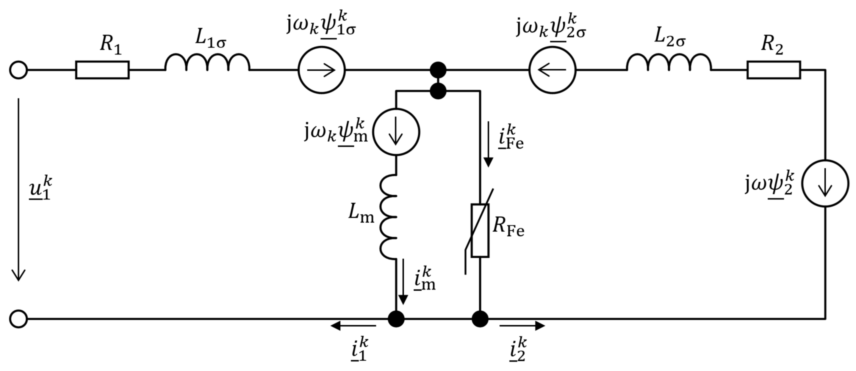
The IM traditional T-equivalent circuit can be augmented to include the effect of the iron losses (Figure 1). In this case, the losses are considered load-independent. In Figure 1, the symbols ${\underset{\_}{\psi }}_1$, ${\underset{\_}{\psi }}_2$, and ${\underset{\_}{\psi }}_{\mathrm{m}}$ represent the stator, rotor, and magnetizing flux linkage space vectors, respectively; ${\underset{\_}{u}}_1$ represents the stator voltage space vector; ${\underset{\_}{i}}_1$, ${\underset{\_}{i}}_2$, ${\underset{\_}{i}}_{\mathrm{m}}$, and ${\underset{\_}{i}}_{\mathrm{Fe}}$ represent the stator, rotor, magnetizing, and equivalent iron loss current space vectors, respectively; R₁, R₂, and R_Fe denote the stator, rotor, and equivalent iron loss resistance, respectively; ω_k is the electrical angular speed of the general reference frame; ω is the rotor electrical angular speed; L_m is the magnetizing inductance; and the symbol j represents an imaginary unit (j² = −1). A short-circuited rotor is considered; therefore, the rotor voltage equals zero. The stator inductance L₁ is defined as L₁ = L_m + L_1σ, where L_1σ is the stator leakage inductance and the rotor inductance L₂ is defined as L₂ = L_m + L_2σ, where L_2σ is the rotor leakage inductance.

The superscript k denotes that the space vectors are expressed in an arbitrary reference frame. The two specific reference frames used in this paper are the stator-fixed (real and imaginary axis denoted as α and β, respectively) and rotor flux vector-attached (real and imaginary axis denoted as d and q, respectively) reference frames.

2.1. Full-Order State-Space Model with Included Effect of Iron Losses

For modeling IM with the included effect of iron losses, the full-order state-space model in the stationary αβ reference frame with the current space vector, magnetizing flux space vector, and rotor flux space vector components as state variables can be used [45]. The model is deductible from Figure 1 and can be expressed mathematically as

$$\dot{x}=Ax+Bu,$$

(1)

where

$$A=\left(\begin{array}{cccccc}{a}_1& 0& a_2& 0& a_3& 0\\ 0& a_1& 0& a_2& 0& a_3\\ R_{\mathrm{Fe}}& 0& a_4& 0& {\tau }_{\mathrm{Fe}\sigma }^{-1}& 0\\ 0& R_{\mathrm{Fe}}& 0& a_4& 0& {\tau }_{\mathrm{Fe}\sigma }^{-1}\\ 0& 0& {\tau }_{\mathrm{r}\sigma }^{-1}& 0& -{\tau }_{\mathrm{r}\sigma }^{-1}& -\omega \\ 0& 0& 0& {\tau }_{\mathrm{r}\sigma }^{-1}& \omega & -{\tau }_{\mathrm{r}\sigma }^{-1}\end{array}\right),$$

(2)

$$B={\left(\begin{array}{cccccc}\frac{1}{L_{1\sigma }}& 0& 0& 0& -\frac{1}{L_{1\sigma }}& 0\\ 0& \frac{1}{L_{1\sigma }}& 0& 0& 0& -\frac{1}{L_{1\sigma }}\\ 0& 0& 0& 0& 1& 0\\ 0& 0& 0& 0& 0& 1\\ 0& 0& 1& 0& 0& 0\\ 0& 0& 0& 1& 0& 0\end{array}\right)}^{\mathrm{T}},$$

(3)

$$x={\left(\begin{array}{cccccc}{i}_{1\alpha }& i_{1\beta }& {\psi }_{\mathrm{m}\alpha }& {\psi }_{\mathrm{m}\beta }& {\psi }_{2\alpha }& {\psi }_{2\beta }\end{array}\right)}^{\mathrm{T}},$$

(4)

$$u={\left(\begin{array}{cccccc}{u}_{1\alpha }& u_{1\beta }& 0& 0& 0& 0\end{array}\right)}^{\mathrm{T}},$$

(5)

and where ${\tau }_{\mathrm{r}\sigma }=L_{2\sigma }/R_2$, ${\tau }_{\mathrm{Fe}\sigma }=L_{2\sigma }/R_{\mathrm{Fe}}$, $a_1=-\left(R_1+R_{\mathrm{Fe}}\right)/L_{1\sigma }$, $a_2=L_2/\left(L_{1\sigma }{L}_{\mathrm{m}}{\tau }_{\mathrm{Fe}\sigma }\right)$, $a_3=-1/\left(L_{1\sigma }{\tau }_{\mathrm{Fe}\sigma }\right)$, $a_4=-L_{1\sigma }{a}_2^{\prime }$.

The electromechanical torque and the motion equation, respectively, are considered in the form

$$T=\frac{3}{2}{p}_{\mathrm{p}}\frac{1}{L_{2\sigma }}\left({\underset{\_}{\psi }}_2^k\times {\underset{\_}{\psi }}_{\mathrm{m}}^k\right),$$

(6)

$$T-T_{\mathrm{L}}=\frac{J}{p_{\mathrm{p}}}\frac{\mathrm{d}\omega }{\mathrm{d}t},$$

(7)

where p_p is the number of pole-pairs, T is the electromagnetic torque, T_L is the load torque, J is the moment of inertia, and the operator × denotes cross product.

2.2. Full-Order State-Space Model without Iron Losses

For the modeling of the machine without the effect of iron losses, it is convenient to use a model with the stator and rotor flux linkage vector components as state variables. The model in its state-space form can be written as [46]

$$\dot{\mathsf{\xi }}=A^{\prime }\mathsf{\xi }+\mathsf{\upsilon },$$

(8)

where

$$A^{\prime }=\left(\begin{array}{cccc}-\frac{R_1{L}_2}{D}& 0& \frac{R_1{L}_{\mathrm{m}}}{D}& 0\\ 0& -\frac{R_1{L}_2}{D}& 0& \frac{R_1{L}_{\mathrm{m}}}{D}\\ \frac{R_2{L}_{\mathrm{m}}}{D}& 0& -\frac{R_2{L}_1}{D}& -\omega \\ 0& \frac{R_2{L}_{\mathrm{m}}}{D}& \omega & -\frac{R_2{L}_1}{D}\end{array}\right),$$

(9)

$$\mathsf{\xi }={\left(\begin{array}{cccc}{\psi }_{1\alpha }& {\psi }_{1\beta }& {\psi }_{2\alpha }& {\psi }_{2\beta }\end{array}\right)}^{\mathrm{T}},$$

(10)

$$\mathsf{\upsilon }={\left(\begin{array}{cccc}{u}_{1\alpha }& u_{1\beta }& 0& 0\end{array}\right)}^{\mathrm{T}},$$

(11)

and where $D=L_1{L}_2-L_{\mathrm{m}}^2$.

The electromechanical torque is given by

$$T=\frac{3}{2}{p}_{\mathrm{p}}\frac{L_{\mathrm{m}}}{D}\left({\underset{\_}{\psi }}_2^k\times {\underset{\_}{\psi }}_1^k\right).$$

(12)

The equation of motion is the same as (7).

3. Reduced-Order Models for Rotor Flux Estimation Considering Iron Loss Effect

In the FOC strategies, the decoupled regulation of flux-producing and torque-producing current components is done in the synchronously rotating dq system where the electromagnetic quantities become DC values. This paper implements a DFOC where the transformation angle, i.e., the angle between the stationary αβ and rotation dq system, is calculated from the rotor flux linkage vector components. For this purpose, two IM reduced-order models can be used: the so-called IM current and voltage models. Conventionally, these models do not consider the effect of iron losses, contrary to the multiple known full-order models that are based on the respective modification (i.e., placement of the iron loss resistance) of the IM equivalent circuit. Since the reduced-order models that consider the iron losses are not often mentioned in the literature, their derivation is, for convenience, presented in the following subsections.

3.1. Current Model with Included Iron Losses

The model will be derived in an arbitrary reference frame and then concretized to αβ and dq reference frames. Using Figure 1, the rotor voltage equation and the rotor flux linkage vector equation, respectively, can be expressed as

$$0=R_2{\underset{\_}{i}}_2^k+\frac{\mathrm{d} {\underset{\_}{\psi }}_2^k}{\mathrm{d}t}+\mathrm{j}({\omega }_k-\omega ) {\underset{\_}{\psi }}_2^k,$$

(13)

$${\underset{\_}{\psi }}_2^k=L_{2\sigma }{\underset{\_}{i}}_2^k+L_{\mathrm{m}}{\underset{\_}{i}}_{\mathrm{m}}^k=L_2{\underset{\_}{i}}_2^k+L_{\mathrm{m}}\left({\underset{\_}{i}}_1^k-{\underset{\_}{i}}_{\mathrm{Fe}}^k\right).$$

(14)

Substituting for the rotor current vector in (13) from (14) yields

$$\frac{\mathrm{d} {\underset{\_}{\psi }}_2^k}{\mathrm{d}t}=\frac{L_{\mathrm{m}}{R}_2}{L_2}{\underset{\_}{i}}_1^{\prime }{}^k-\frac{R_2}{L_2}{\underset{\_}{\psi }}_2^k-\mathrm{j}({\omega }_k-\omega ) {\underset{\_}{\psi }}_2^k,$$

(15)

where ${\underset{\_}{i}}_1^{\prime }{}^k={\underset{\_}{i}}_1^k-{\underset{\_}{i}}_{\mathrm{Fe}}^k$. If the stator-fixed reference frame is considered (ω_k = 0), the model becomes

$$\frac{\mathrm{d} {\underset{\_}{\psi }}_2^{\alpha \beta }}{\mathrm{d}t}=\frac{L_{\mathrm{m}}{R}_2}{L_2}{\underset{\_}{i}}_1^{\prime }{}^{\alpha \beta }-\frac{R_2}{L_2}{\underset{\_}{\psi }}_2^{\alpha \beta }+\mathrm{j}\omega {\underset{\_}{\psi }}_2^{\alpha \beta }.$$

(16)

On the other hand, choosing the rotor flux linkage vector-attached dq reference frame, the steady-state expression for the rotor flux magnitude and slip frequency, respectively, can be expressed as

$${\psi }_2=L_{\mathrm{m}}{i}_{1d}^{\prime },$$

(17)

$${\omega }_{\mathrm{sl}}=\frac{L_{\mathrm{m}}{R}_2}{L_2}\frac{i_{1q}^{\prime }}{{\psi }_{2d}},$$

(18)

where ${\psi }_2={\psi }_{2d}=\left|{\underset{\_}{\psi }}_2\right|$, $i_{1d}^{\prime }=i_{1d}-i_{\mathrm{Fe}d}$, and $i_{1q}^{\prime }=i_{1q}-i_{\mathrm{Fe}q}$.

3.2. Voltage Model with Included Iron Losses

The model will be derived in the αβ reference frame. According to Figure 1, the stator flux linkage vector can be expressed as

$${\underset{\_}{\psi }}_1^k=L_{1\sigma }{\underset{\_}{i}}_1^k+L_{\mathrm{m}}{\underset{\_}{i}}_{\mathrm{m}}^k=L_1{\underset{\_}{i}}_1^k+L_{\mathrm{m}}\left({\underset{\_}{i}}_2^k-{\underset{\_}{i}}_{\mathrm{Fe}}^k\right).$$

(19)

Substituting for the rotor current vector in (14) from (19) and considering the stator-fixed reference frame yields

$${\underset{\_}{\psi }}_2^{\alpha \beta }=\frac{L_2}{L_{\mathrm{m}}}\left({\underset{\_}{\psi }}_1^{\alpha \beta }-L_1\sigma {\underset{\_}{i}}_1^{\alpha \beta }\right)+L_{2\sigma }{\underset{\_}{i}}_{\mathrm{Fe}}^{\alpha \beta },$$

(20)

where $\sigma =1-L_{\mathrm{m}}^2/L_1{L}_2$ is the leakage factor. The stator flux linkage vector is obtained as

$${\underset{\_}{\psi }}_1^{\alpha \beta }={{\displaystyle \int }}_0^t\left({\underset{\_}{u}}_1^{\alpha \beta }-R_1{\underset{\_}{i}}_1^{\alpha \beta }\right)\mathrm{d}\tau .$$

(21)

3.3. Implementation of Current and Voltage Model into Discrete System

The real-time motor control algorithm is implemented either on DSP or FPGA. Therefore, the continuous mathematical models must be solved numerically. The current model (16) represents a complicated set of coupled differential equations when resolved into the real and imaginary parts. Therefore, as mentioned in the introduction, one of the aims of this paper is to compare the influence of the solver and sampling time selection on the accuracy of the DFOC and MRAS algorithms. The following numerical methods are considered: the forward Euler method (FWEM), the trapezoidal rule (TR), and the fourth-order Runge–Kutta method (RK4). These approaches are well-known algorithms for the solution of ordinary differential equations (ODE); therefore, they will be described here only briefly.

Let us consider a first-order ODE in the form

$$\dot{y}\left(t\right)=f \left(t,y\left(t\right)\right),\hspace{1em}\hspace{1em}y\left(t_0\right)=y_0.$$

(22)

The most straightforward approach for numerically solving (22) is the forward Euler method given by the rule (a fixed step Δt is assumed) [47]

$$y_i=y_{i-1}+\Delta t\cdot f\left(t_{i-1},y_{i-1}\right).$$

(23)

The method is first order, making it computationally undemanding but with limited accuracy and stability. An improvement can be achieved by using the trapezoidal rule: at the cost of one extra function evaluation, we improve the order of the method by one. The rule is given by the following formula [47]

$$y_i=y_{i-1}+\frac{\Delta t}{2}\left[f\left(t_{i-1},y_{i-1}\right)+f\left(t_i,y_i\right)\right].$$

(24)

The last numerical approach considered in this paper is the popular fourth-order Runge–Kutta method, which can be summarized as [47]

$$y_i=y_{i-1}+\frac{1}{6}\Delta t\left(k_1+2k_2+2k_3+k_4\right),$$

(25)

$$k_1=f\left(t_{i-1},y_{i-1}\right),$$

(26)

$$k_2=f\left(t_{i-1}+\frac{1}{2}\Delta t,y_{i-1}+\frac{1}{2}\Delta t\cdot k_1\right),$$

(27)

$$k_3=f\left(t_{i-1}+\frac{1}{2}\Delta t,y_{i-1}+\frac{1}{2}\Delta t\cdot k_2\right),$$

(28)

$$k_4=f\left(t_i, y_{i-1}+\Delta t\cdot k_3\right).$$

(29)

4. Modelling of Inverter Nonlinearities

A proper inverter model is needed to assess the effect of the IGBT inverter nonlinearities on the DFOC and MRAS algorithms. By a nonlinear inverter behavior, we mean the semiconductor’s finite turn-on and turn-off times, the voltage drop across the devices, and necessary protective time, i.e., dead-time inserted by the microcontroller or the transistor driver [48]. Since a 400 V IM drive is considered, the voltage drop across the devices will be neglected.

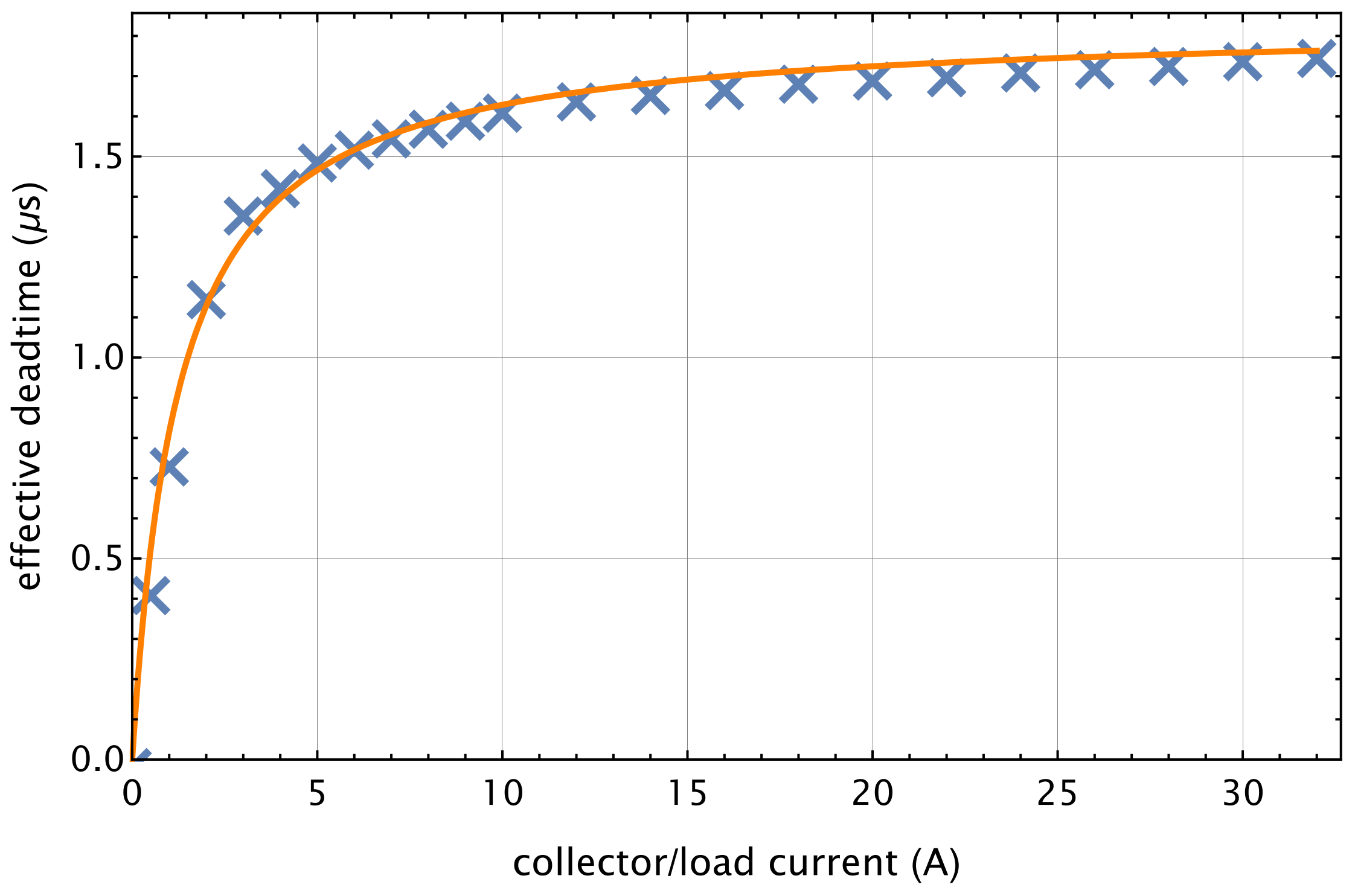
Let us consider the most common space-vector modulation (SVM) with a fixed switching period T_PWM. By a simple graphical analysis, it can be concluded that the turn-on time T_on increases and the turn-off time T_off decreases the distortion given by the dead-time T_dt [48]. Therefore, it is convenient to define the so-called effective dead-time as

$$T_{\mathrm{eff}}\left(i_x\right)=T_{\mathrm{dt}}+T_{\mathrm{on}}\left(i_x\right)-T_{\mathrm{off}}\left(i_x\right) x=a, b, c,$$

(30)

where it is assumed that the turn-on and turn-off times are only the function of the load current, and the symbols a, b, c denote the respective inverter leg. A direct inverter measurement can be performed to easily determine the dependence of the effective deadtime on the load current. The resulting characteristics can then be implemented as a look-up table or analytically approximated using the expression

$$T_{\mathrm{eff}}\left(i_x\right)=\frac{m}{c_1\left|i_x\right|+c_2}+n,$$

(31)

where c₁, c₂, m, and n are parameters. The measured and approximated dependence of the effective deadtime on the collector/load current of an IGBT module SKM100GB12T4 from SEMIKRON that is used later in the simulation model is depicted in Figure 2 The actual deadtime is selected as 2 µs.

Let us assume that, within SVM, the standard up-down counters are utilized with the top value normalized to one and the period of the signal equal to T_PWM. Moreover, suppose that the comparator, which compares the counter with the reference compare value, outputs a logical one when a match during up-count occurs and logical zero when a match during a down-count occurs. Then, to model the voltage distortion of an ideal inverter, the reference compare value $d_x^{*}$ for the respective VSI leg (i.e., the SVM output) must be adjusted as

$$d_x^{\prime }=d_x^{*}+d_{\mathrm{dist}\left(x\right)} x=a,b,c,$$

(32)

where

$$d_{\mathrm{dist}\left(x\right)}=\frac{T_{\mathrm{eff}\left(x\right)}}{T_{\mathrm{PWM}}}\mathrm{sgn}\left(i_x\right) x=a,b,c.$$

(33)

The following well-known expression can be utilized for the reconstruction of the actual phase voltage of a wye-connected machine:

$$\left[\begin{array}{c}{u}_{\mathrm{a}}\\ u_{\mathrm{b}}\\ u_{\mathrm{c}}\end{array}\right]=\frac{1}{3}{U}_{\mathrm{DC}}\left[\begin{array}{ccc}2& -1& -1\\ -1& 2& -1\\ -1& -1& 2\end{array}\right]\left[\begin{array}{c}{S}_{\mathrm{a}}\\ S_{\mathrm{b}}\\ S_{\mathrm{c}}\end{array}\right],$$

(34)

where u_a, u_b, and u_c are the respective motor phase voltages and S_a, S_b, and S_c are the logical switching variables (1—high-side switch in the respective inverter leg is on, 0—low-side switch in the respective inverter leg is on) from the comparator. Knowing the effective deadtime of each VSI leg, the nonideal inverter can be modeled using (32)–(34).

5. Measuring, Modelling, and Compensation of Iron Losses

The last phenomenon examined in this paper is the influence of iron losses on the DFOC and MRAS performance. This section describes the integration of the iron losses measured on a real machine either into a machine or DFOC model. According to Figure 1, the equivalent iron loss current in an arbitrary reference frame can be expressed as

$${\underset{\_}{i}}_{\mathrm{Fe}}^k=\frac{{\underset{\_}{u}}_{\mathrm{m}}^k}{R_{\mathrm{Fe}}},$$

(35)

where ${\underset{\_}{u}}_{\mathrm{m}}^k$ is the voltage across the magnetizing (parallel) branch. The power dissipated in the fictitious iron loss resistance can be expressed as

$$P_{\mathrm{Fe}}=\frac{3}{2}\Re \left\{{\underset{\_}{u}}_{\mathrm{m}}^k{\overline{i}}_{\mathrm{Fe}}^k\right\},$$

(36)

where ${\overline{i}}_{\mathrm{Fe}}^k$ denotes the complex conjugate of the equivalent iron loss current. Substituting (35) into (36), the iron loss resistance is obtained as

$$R_{\mathrm{Fe}}=\frac{3}{2}\frac{u_{\mathrm{m}}^2}{P_{\mathrm{Fe}}}.$$

(37)

The iron loss current in the stationary system is obtained using (37) to substitute for the equivalent iron loss resistance in (35):

$${\underset{\_}{i}}_{\mathrm{Fe}}^{\alpha \beta }=\frac{2}{3}{P}_{\mathrm{Fe}}\frac{{\underset{\_}{u}}_{\mathrm{m}}^{\alpha \beta }}{u_{\mathrm{m}}^2}.$$

(38)

Within the model of the machine, the voltage across the magnetizing branch can be obtained directly using the magnetizing flux vector time derivative. In the control algorithm, the voltage can be approximately calculated as

$${\underset{\_}{u}}_{\mathrm{m}}^{\alpha \beta }={\underset{\_}{u}}_1^{\alpha \beta }-R_1{\underset{\_}{i}}_1^{\alpha \beta }-\mathrm{j}{\omega }_{\mathrm{s}}{L}_{1\sigma } {\underset{\_}{i}}_1^{\alpha \beta }.$$

(39)

Equation (39) supposes a steady-state operation and considers the fundamental wave only.

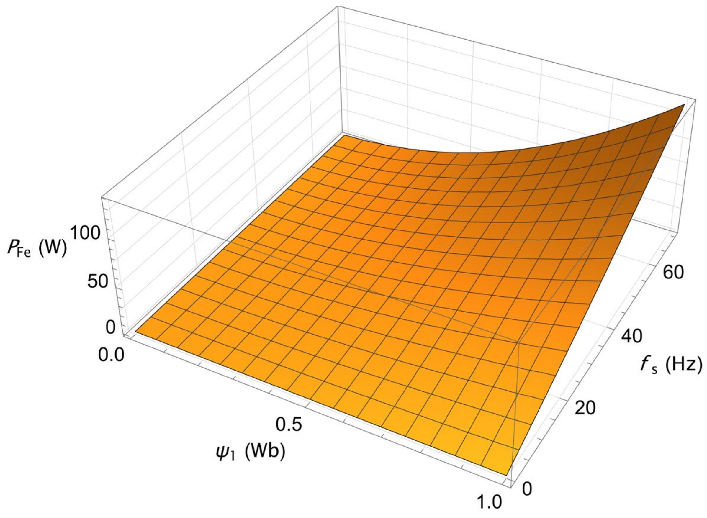
Iron Losses Measurement and Model Fitting

The iron losses can be obtained by a series of no-load tests at various fundamental supply frequencies. The separation procedure based on the IEC standard (IEC 60034-2-1: 2014 [49]) can then be used for the loss calculation [50]. For the measurement, the inverter is programmed to generate a fundamental voltage at a given frequency and magnitude that corresponds to the reference stator flux linkage vector magnitude (obtained from the voltage model). For the iron loss modeling, the following analytical function can be used [4]

$$P_{\mathrm{Fe}}=\frac{f_{\mathrm{s}}^2{\psi }_1^2+\kappa f_{\mathrm{s}}{\psi }_1^n}{R_{\mathrm{Fe}0}},$$

(40)

where f_s is the fundamental supply frequency, ψ₁ is the stator flux linkage amplitude, and κ, n, and R_Fe0 are the model parameters. Figure 3 shows (40) fitted to the measured losses of a 3.6 kW IM drive (nameplate data and nominal model parameters are given in

Table A1. Induction motor nameplate data and mathematical model parameters.

Nameplate Data		Mathematical Model Parameters
Nominal power	3.6 kW	Stat. resistance	1.688 Ω
Nominal voltage	380 V	Rot. resistance	3.685 Ω
Nominal current	11.5 A	Stat. leak inductance	0.012 H
Nominal speed	935 min−1	Rot. leak. inductance	0.013 H
Number of poles	6	Mag. inductance	0.175 H
Winding connection	Y	Iron core resistance	520 Ω

).

6. Improved MRAS Estimators with Included Effect of Iron Losses

The philosophy behind MRAS estimators is that the estimated parameter should somehow influence the adaptive model. In the case of the active power MRAS, the adaptive model directly depends on the stator resistance, making it suitable for the stator resistance estimation. Contrary to that, the adaptive model of the reactive power MRAS used for the rotor resistance estimation depends on the rotor resistance indirectly. By indirect dependence, we mean that the model utilizes quantities affected by the rotor resistance, i.e., the calculated slip speed and d and q-axis current components.

Since most of the MRAS algorithms for the parameter estimation proposed in the literature do not include the effect of iron losses, this section presents improved stator and rotor resistance estimators based on the active (P-MRAS) reactive (Q-MRAS) power.

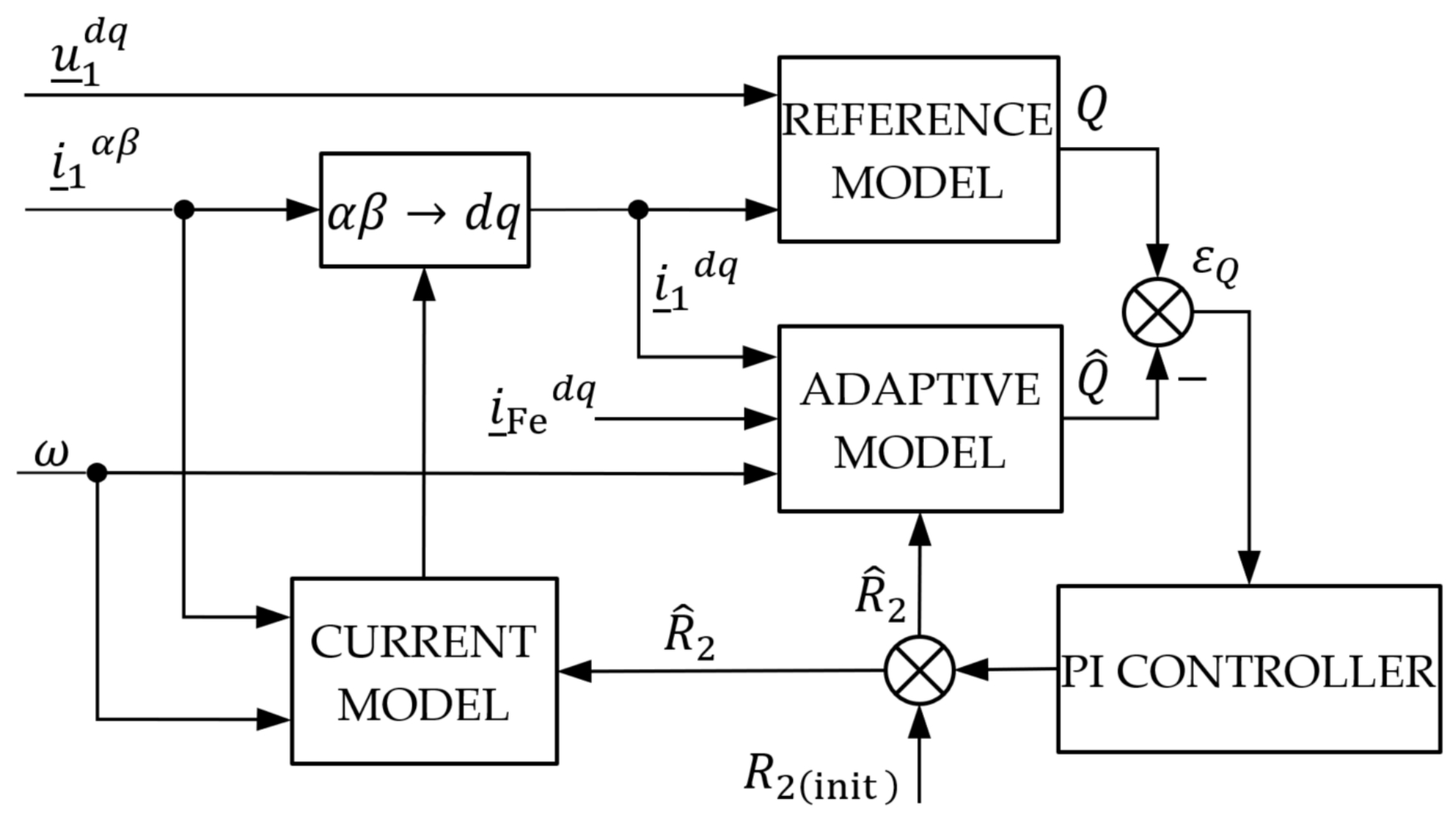
6.1. Improved Reactive Power MRAS with Included Effect of Iron Losses

The reference model of the popular and widely used Q-MRAS for the rotor resistance (or inverse rotor time constant) estimation is given by [10,11,12,13,14]

$$Q=\Im \left\{{\underset{\_}{u}}_1^{dq}{\overline{i}}_1^{dq}\right\}=u_{1q}{i}_{1d}-u_{1d}{i}_{1q},$$

(41)

where ${\overline{i}}_1^{dq}$ denotes the conjugated current space vector. Using (20) transformed into the dq reference frame, the stator flux linkage vector can be obtained as

$${\underset{\_}{\psi }}_1^{dq}=\frac{L_{\mathrm{m}}}{L_2}{\underset{\_}{\psi }}_2^{dq}+L_1\sigma {\underset{\_}{i}}_1^{dq}-\frac{L_{2\sigma }{L}_{\mathrm{m}}}{L_2}{\underset{\_}{i}}_{\mathrm{Fe}}^{dq}.$$

(42)

The stator voltage equation in the dq reference frame can be written as

$${\underset{\_}{u}}_1^{dq}=R_1{\underset{\_}{i}}_1^{dq}+\frac{\mathrm{d}{\underset{\_}{\psi }}_1^{dq}}{\mathrm{d}t}+\mathrm{j}{\omega }_{\mathrm{s}}{\underset{\_}{\psi }}_1^{dq}.$$

(43)

By substituting (41) into (43) and considering the steady-state operation, we obtain

$${\underset{\_}{u}}_1^{dq}=R_1{\underset{\_}{i}}_1^{dq}+\mathrm{j}{\omega }_s\left(\frac{L_{\mathrm{m}}}{L_2}{\underset{\_}{\psi }}_2^{dq}+L_1\sigma {\underset{\_}{i}}_1^{dq}-\frac{L_{2\sigma }{L}_{\mathrm{m}}}{L_2}{\underset{\_}{i}}_{\mathrm{Fe}}^{dq}\right).$$

(44)

Separating (44) into the real and imaginary parts, respectively, while considering that ${\psi }_{2d}=L_{\mathrm{m}}\left(i_{1d}-i_{\mathrm{Fe}d}\right)$ and ψ_2q = 0, the adaptive model is finally obtained as

$$\widehat{Q}={\omega }_{\mathrm{s}}\left[L_1\sigma \left(i_{1d}^2+i_{1q}^2\right)+\frac{L_{\mathrm{m}}}{L_2}\left(L_{\mathrm{m}}{i}_{1d}^2-L_2{i}_{\mathrm{Fe}d}{i}_{1d}-L_{2\sigma }{i}_{\mathrm{Fe}q}{i}_{1q}\right)\right].$$

(45)

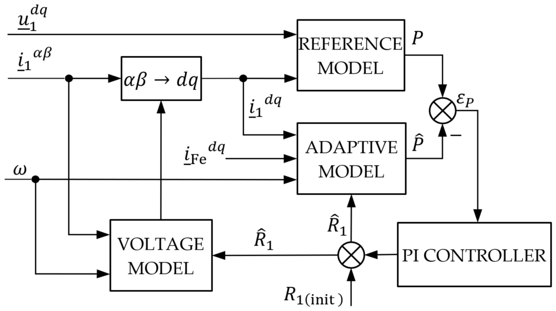
The synchronous speed is calculated as the sum of the measured speed and estimated slip speed (Equation (18)). The error for the rotor resistance adaptation mechanism is given by

$${\epsilon }_Q=Q-\widehat{Q}.$$

(46)

The estimated rotor resistance is then the output of the PI controller, i.e.,

$${\widehat{R}}_2=K_{\mathrm{p}Q}{\epsilon }_Q+K_{\mathrm{i}Q}{{\displaystyle \int }}_0^t{\epsilon }_Q\mathrm{d}\tau +R_{2\left(\mathrm{init}\right)},$$

(47)

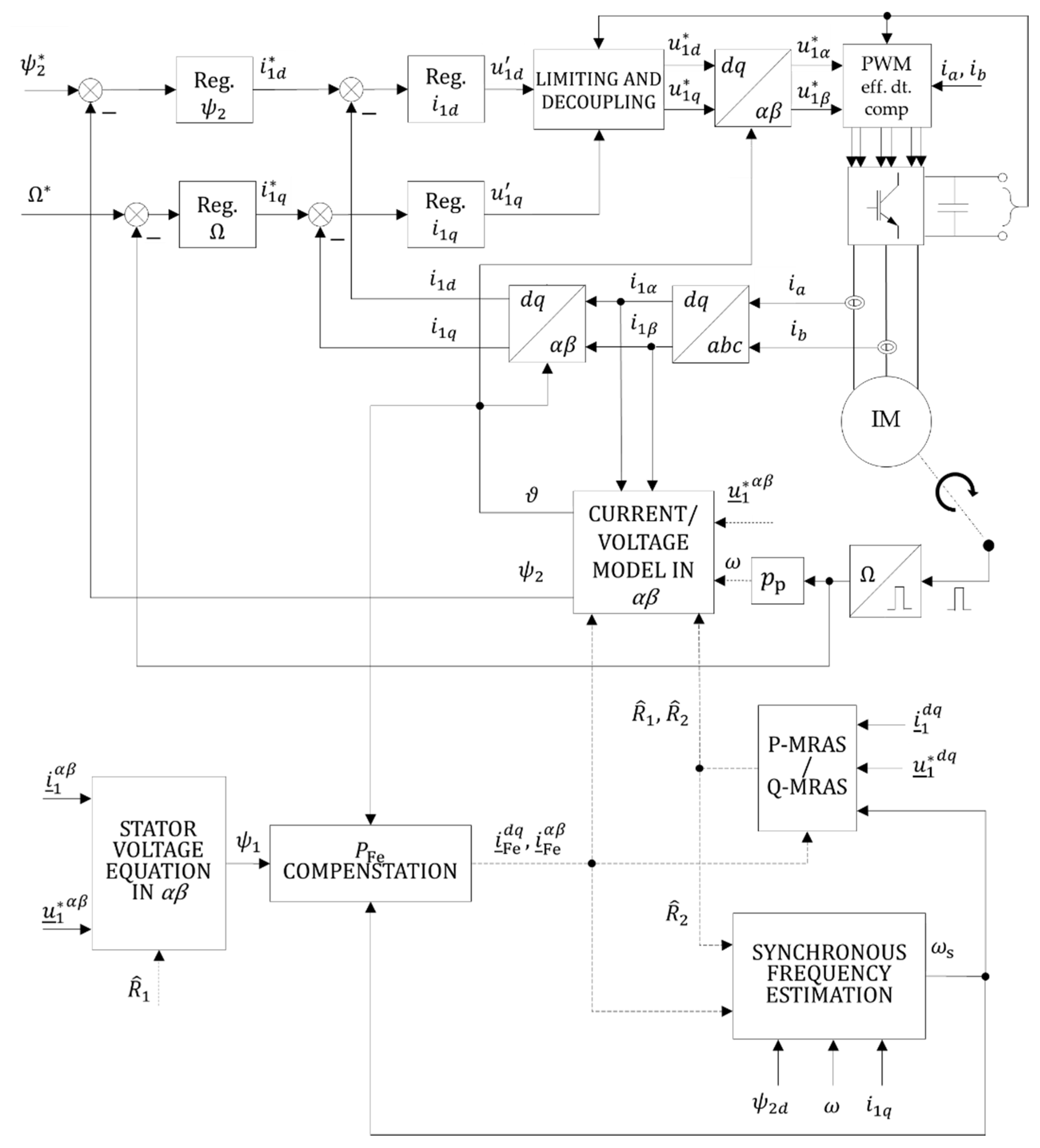
where R_2(init) is the initial rotor resistance. The block diagram of the Q-MRAS estimator with the included iron loss effect is presented in Figure 4. Due to its dependency on the rotor resistance, the current model is used for the transformation angle calculation.

6.2. Improved Active Power MRAS with Included Effect of Iron Losses

The reference model of the P-MRAS is given by [10,29,30]

$$P=\Re \left\{{\underset{\_}{u}}_1^k{\overline{i}}_1^k\right\}=u_{1d}{i}_{1d}+u_{1q}{i}_{1q}.$$

(48)

Separating (44) into the real and imaginary parts, respectively, and substituting the resulting expression into (48) while considering that ${\psi }_{2d}=L_{\mathrm{m}}\left(i_{1d}-i_{\mathrm{Fe}d}\right)$ and ψ_2q = 0, the adaptive model is obtained as

$$\widehat{P}=R_1\left(i_{1d}^2+i_{1q}^2\right)+{\omega }_{\mathrm{s}}{L}_{\mathrm{m}}\left(\frac{L_{\mathrm{m}}}{L_2}{i}_{1d}{i}_{1q}+\frac{L_{2\sigma }}{L_2}{i}_{\mathrm{Fe}q}{i}_{1d}-i_{\mathrm{Fe}d}{i}_{1q}\right).$$

(49)

The error for the rotor resistance adaptation mechanism is calculated as

$${\epsilon }_P=P-\widehat{P}.$$

(50)

The estimated stator resistance is then the output of the PI controller, i.e.,

$${\widehat{R}}_1=K_{\mathrm{p}P}{\epsilon }_P+K_{\mathrm{i}P}{{\displaystyle \int }}_0^t{\epsilon }_P\mathrm{d}\tau +R_{1\left(\mathrm{init}\right)},$$

(51)

where R_1(init) is the initial stator resistance. The block diagram of the modified P-MRAS estimator is presented in Figure 5. Here, the voltage model is selected for the transformation angle calculation due to its dependency on the stator resistance.

7. Simulation Results

As mentioned in the introduction, this paper aims to examine selected phenomena that impair the performance of motor control algorithms. These include inverter nonlinearity, iron losses, ODE solver type, and sampling time. The presented results are based on simulations in MATLAB/Simulink because:

• It is not possible to fully separate the influence of the aforementioned adverse effects in an actual application.
• Many additional nonlinearities and imperfections are present in a real system.
• The exact system parameters are usually not known.

7.1. Simulation Setup Description

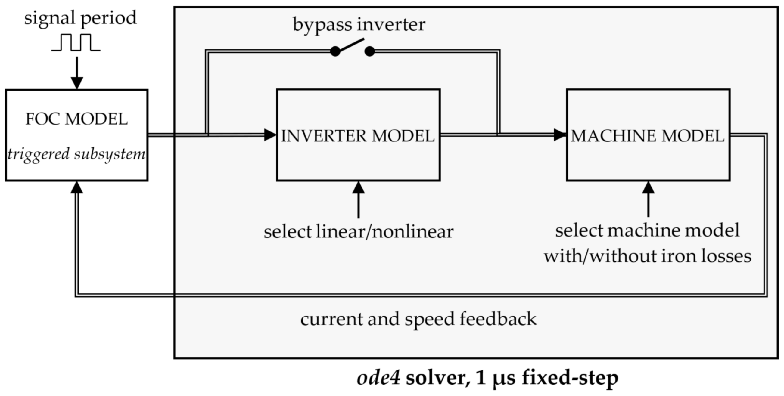
The principal block diagram of the Simulink model is depicted in Figure 6. The model permits to switch between the machine model with the iron losses (1)–(6) and without the iron losses (8)–(12). The simulated machine is a 3.6 kW IM whose nameplate data and nominal model parameters are given in Table A1. The iron losses are measured and implemented in accordance with Section 5. Both machine models are simulated using the ode4 solver with a fixed-step size equal to 1 µs.

The inverter model is implemented using SVM in a linear mode with the possibility to simulate the inverter nonlinearity using the approach described in Section 4. The switching frequency is selected as 10 kHz. Again, the inverter is simulated using the ode4 solver with a fixed-step size 1 µs.

The block diagram of the considered DFOC scheme is depicted in Figure 7. The advantage of the presented DFOC scheme is the ability to estimate the stator and rotor resistance variation in the presence of iron losses using improved estimators. The disadvantage is that machine iron losses and nonlinear inverter characteristics need to be measured and implemented for proper functionality, and additional PI controllers have to be tuned. Moreover, in an actual application, the DFOC performance can be further improved by respecting the saturation of the main flux paths.

The FOC model is simulated as a triggered subsystem to mimic the fact that motor control algorithms are implemented on a discrete system. The type of the ODE solver (FWEM or TR) is selected by setting the appropriate integration method in the Discrete-Time Integrator blocks. The RK4 method is implemented using the MATLAB Function Block. Within FOC, it is also possible to switch between the voltage model and the current model, both either with or without the iron losses. Concerning the MRAS testing, the Q-MRAS is tested with the current model, and the P-MRAS is tested with the voltage model active.

The initial gains of the PI controllers within the FOC were calculated using the optimum modulus method. The obtained values were further adjusted to improve the controllers’ performance. The gains of the adaptive PI controllers inside the MRAS estimators were tuned experimentally (the values are given in

Table A2. P-MRAS and Q-MRAS adaptive PI controller gain values.

P-MRAS		Q-MRAS
Proportional gain	10−4	Proportional gain	10−6
Integral gain	0.25	Integral gain	0.05

).

7.2. Influence of VSI Nonlinearities on P-MRAS and Q-MRAS Estimators

This simulation series aims to examine the influence of the inverter nonlinearity on the accuracy of the MRAS estimators. The simulation setup is as follows:

• The IM model is implemented without iron losses using (8)–(12).
• The sample time of the FOC model (triggered subsystem) is selected as 100 µs (synchronized with PWM).
• The rotor flux is set to a nominal value.

Within FOC control strategies, it is common that a reference voltage (i.e., the input to the modulator) is utilized instead of a measured voltage. However, when this approach is used, inverter nonlinearities should be compensated appropriately. The influence of the nonideal inverter on the estimation of the stator flux linkage vector $\alpha$ component using (21) is depicted in Figure 8. As expected, the nonlinearities become more significant at small speeds and light loads (Figure 8a). At higher speeds and loads (Figure 8b), the relative influence of the distorting voltage vector decreases.

Figure 9 shows the influence of the nonlinear inverter behavior on the stator resistance (Figure 9a) and rotor resistance (Figure 9b) estimation. The resistances are presented in a per-unit system (indicated by lower-case letters), with the base impedance selected as the ratio of the machine nominal phase voltage and current.

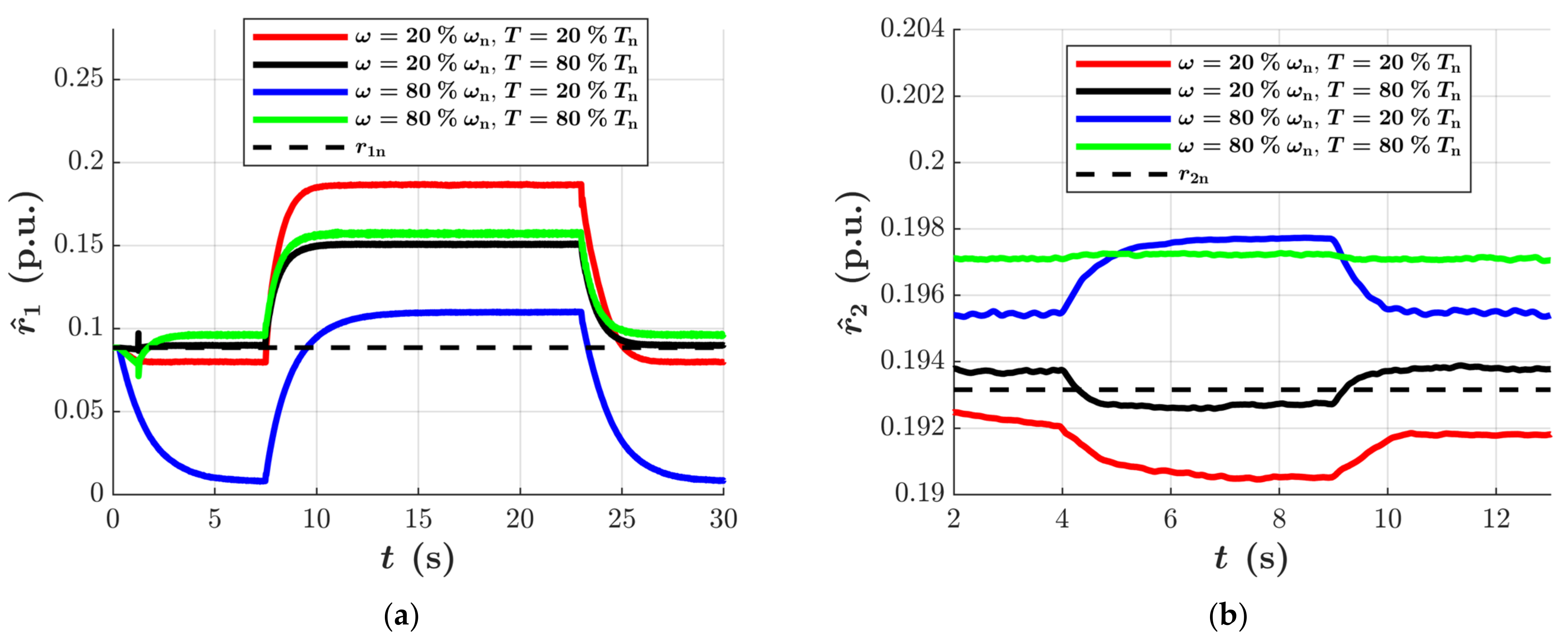
In the case of the stator resistance, the voltage nonlinearity significantly impacts the estimation accuracy because the distorted voltage is utilized not only by the voltage model but also by the P-MRAS reference and adaptive models. The wrong estimate during the low-speed and light-load operation is given mainly by the relatively low ratio of the fundamental and distorting voltage vector. At higher speeds, the relative influence of the stator resistance on the FOC performance decreases, which also impairs the estimator’s performance.

The rotor resistance estimation depicted in Figure 9b is, overall, much less sensitive to the voltage distortion because the stator voltage influences the estimator only through the Q-MRAS reference and adaptive models. Like the P-MRAS, the resulting estimates are influenced by the voltage nonlinearity mainly during low-speed and high-speed low-load operations.

7.3. Influence of Iron Losses on P-MRAS and Q-MRAS Estimators

The simulation setup is as follows:

• The IM model is implemented with iron losses using (1)–(6).
• The inverter is bypassed, i.e., the machine is supplied by a sinusoidal voltage.
• The FOC model makes it possible to switch between voltage, current, and synchronous speed estimation with and without iron losses.
• The sample time of the FOC model (triggered subsystem) is selected as 10 µs.
• The rotor flux is set to a nominal value.

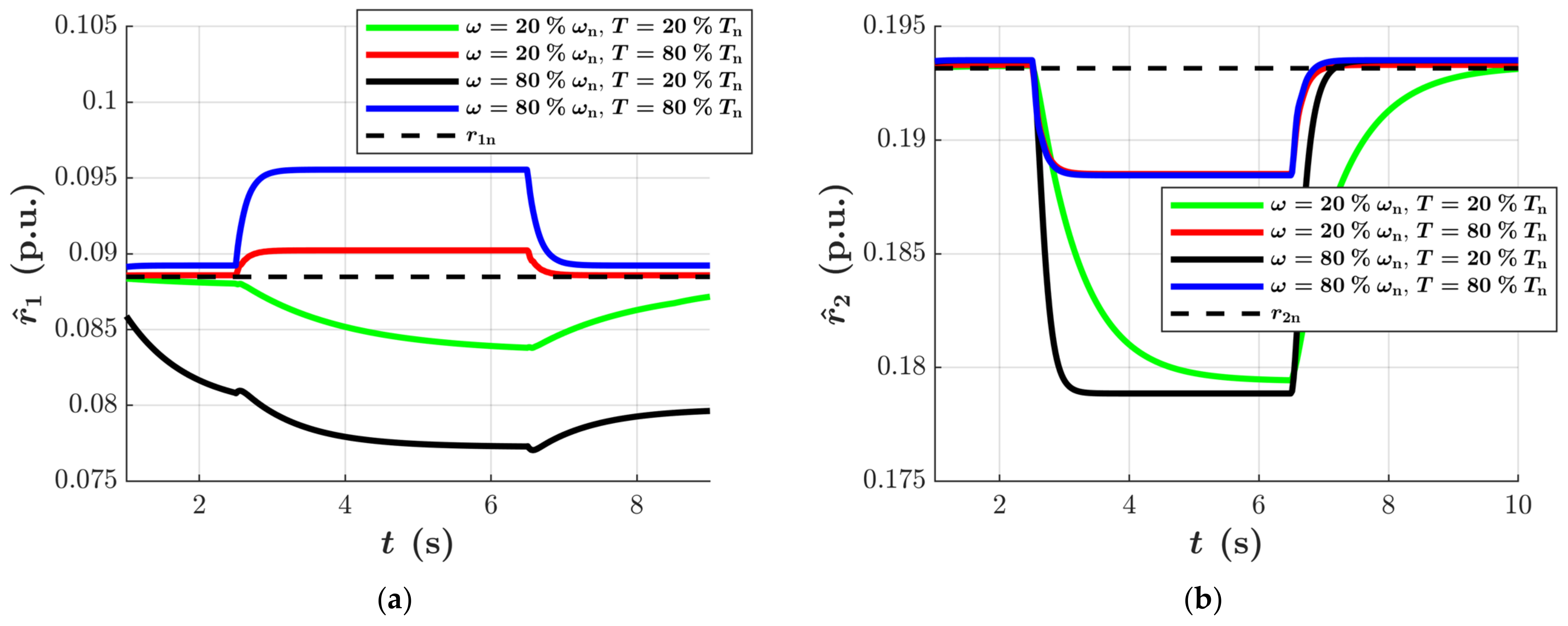
Figure 10 shows the influence of the iron losses on the stator resistance (Figure 10a) and rotor resistance (Figure 10b) estimation. The iron losses are a non-linear phenomenon whose influence on the flux estimation at different speeds and applied load torques is described by complicated functions [42]. Combining the FOC with MRAS creates a complex system where it is complicated to express the influence of the iron losses on the whole system performance by explicit analytical expression. Overall, it can be stated that the iron losses definitely and not negligibly affect the parameter estimation process and that the influences of the speed and load are interconnected. However, in the case of the P-MRAS, the impact of the iron losses on the estimation accuracy is relatively lower compared to the inverter nonlinearity.

7.4. Influence of Discretization and Sampling Time on P-MRAS and Q-MRAS Estimators

The last examined phenomenon is the effect of the discretization and sampling time on the relative error of the estimate. The simulation setup is as follows:

• The IM model is implemented without iron losses using (8)–(12).
• The inverter is bypassed, i.e., the machine is supplied by a sinusoidal voltage.
• The sample time of the FOC model (triggered subsystem) is varied from 10 µs to 300 µs.
• The FWEM and TR are selected by specifying an integration method in the Discrete-Time Integrator blocks used in the DFOC model. The RK4 method is implemented manually using the MATLAB Function block.
• The rotor flux is set to a nominal value.

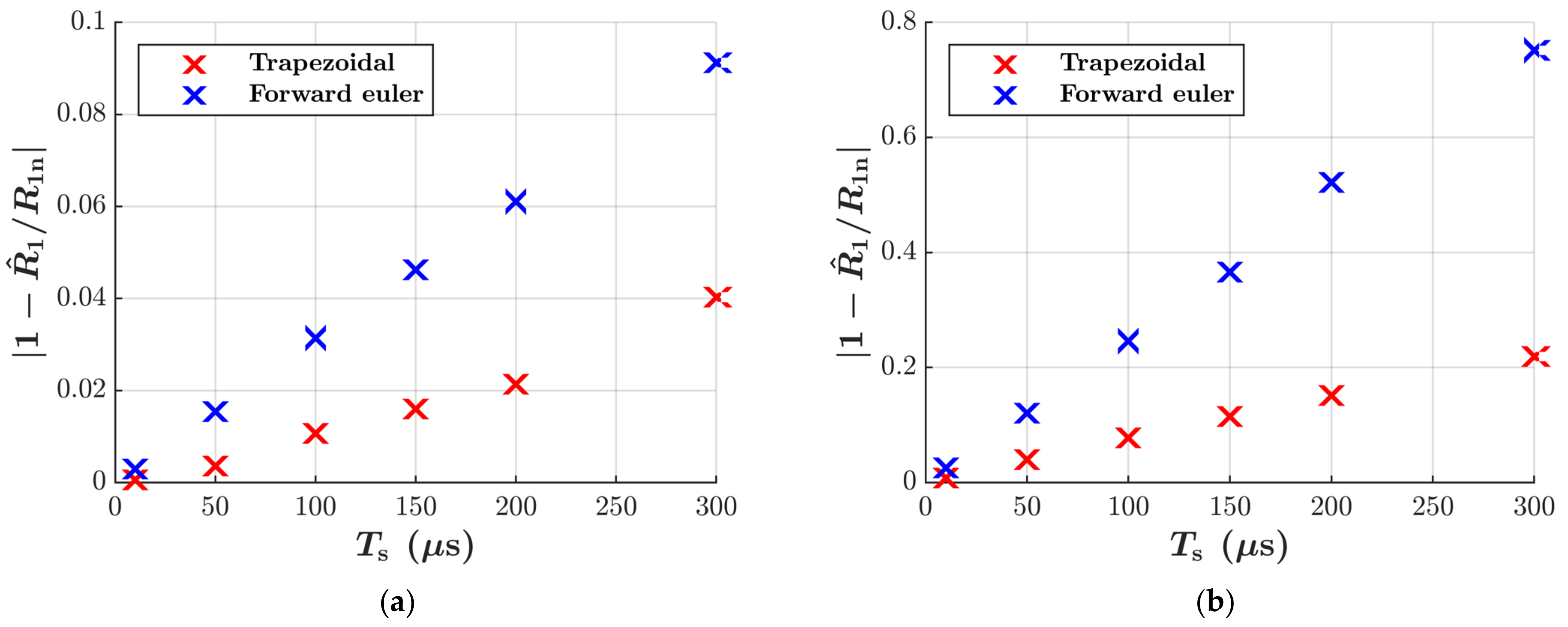
Figure 11 shows the influence of the discretization method and sampling time on the resulting relative error of the stator resistance estimation. As expected, the influence of the discretization method grows with the increasing sampling time. Furthermore, the relative error is much more significant at higher speeds because of the higher fundamental and sampling frequency ratio. Since the order of the trapezoidal method is only one order higher than the Euler method, it should be a preferred choice.

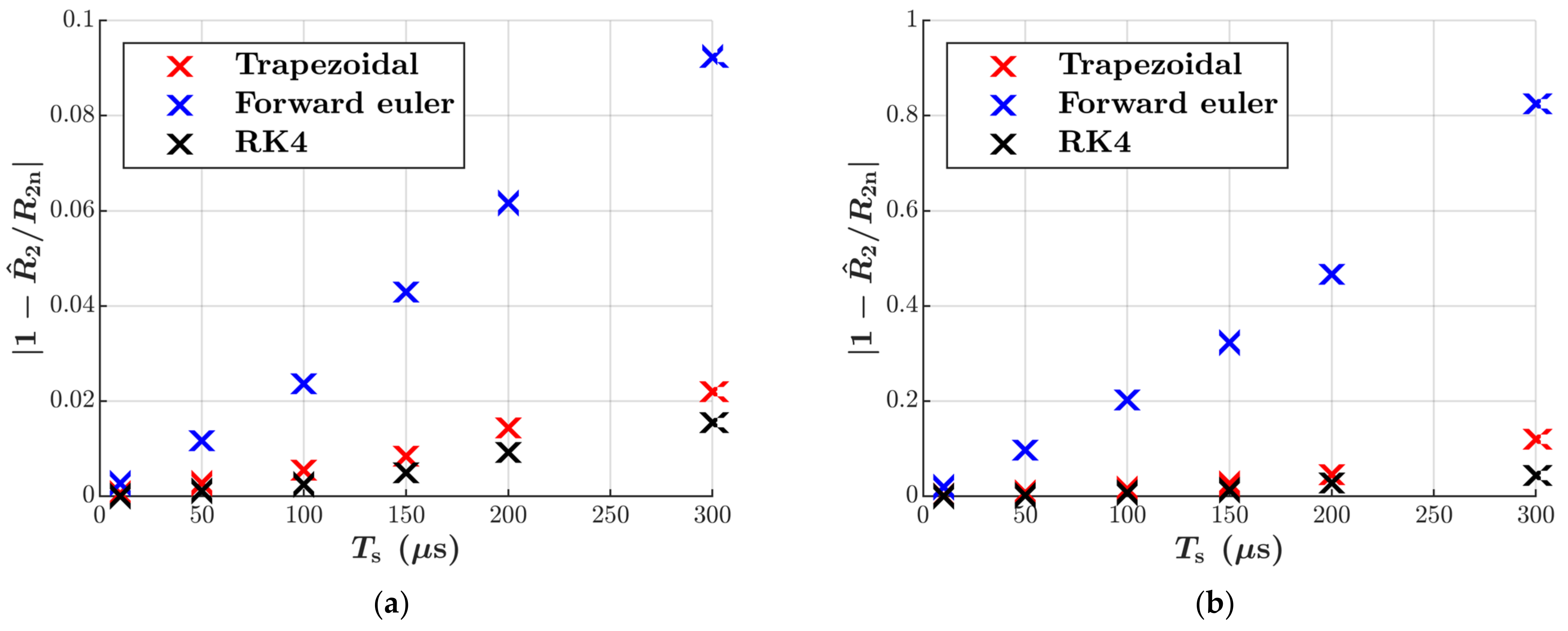
Figure 12 shows the results for the Q-MRAS estimator. Here, because of the current model, the RK4 solver is also tested. The results and conclusions for the TR and FWEM are the same as in the case of Figure 11. The RK4 method can increase the estimation accuracy, especially at higher sampling times. Moreover, it is supposed to maintain higher numerical stability during fast transients.

If hardware with sufficient computational power, such as FPGA or DSP with FPGA, is used in real applications, the FOC performance can be increased by oversampling. However, this might not always be the most cost-effective solution. The sampling time is often tied to the PWM period in medium-power drives operating with the switching frequencies around 10 kHz, which, according to Figure 11 and Figure 12, can deteriorate the accuracy of the MRAS-type estimators.

8. Discussion

This paper investigated three actual application phenomena on the accuracy of the popular Q-MRAS and P-MRAS rotor and stator resistance estimators. The studied adverse effects include inverter nonlinearity, iron losses, ODE solver type, and sampling time selection. The main results and contributions of the paper can be summarized as follows:

• If not adequately accounted for, the inverter nonlinearity has a key influence on the parameter estimation in the case of the P-MRAS and voltage model. The Q-MRAS is also affected by the inaccurate voltage evaluation, but relatively much less.
• The influence of iron losses on the stator and rotor resistance estimation accuracy is investigated using improved reduced-order IM models and improved Q-MRAS and P-MRAS estimators with the included iron losses. The simulation results show that, if not adequately compensated, the nonlinear phenomenon of iron losses impairs the estimation process and leads to inaccurately identified parameters. The error can become quite significant and is comparable for both the stator and rotor resistance estimation.
• Numerical method and sampling time selection can also affect the MRAS-based parameter estimation. When oversampling is impossible, and the drive control system operates with the sampling time around 100 µs, it is recommended to use at least the trapezoidal rule because the improvement compared to Euler’s method is significant. The difference between the Runge–Kutta fourth-order method and the trapezoidal rule is not so pronounced. However, the RK4 method is expected to exhibit better numerical stability.

In the case of the inverter nonlinearity and iron losses, the operating conditions, i.e., the applied load and the rotor speed, represent a complicated mixed influence on the stator and rotor estimation accuracy. The analytical description of the observed would represent a highly complex task due to the nonlinearity of the whole system.

References

- Wang, F.; Zhang, Z.; Mei, X.; Rodríguez, J.; Kennel, R. Advanced Control Strategies of Induction Machine: Field Oriented Control, Direct Torque Control and Model Predictive Control. Energies 2018, 11, 120. [Google Scholar] [CrossRef] [Green Version]
- Wang, K.; Huai, R.; Yu, Z.; Zhang, X.; Li, F.; Zhang, L. Comparison Study of Induction Motor Models Considering Iron Loss for Electric Drives. Energies 2019, 12, 503. [Google Scholar] [CrossRef] [Green Version]
- Hinkkanen, M.; Repo, A.; Luomi, J. Influence of magnetic saturation on induction motor model selection. In Proceedings of the 17th International Conference on Electrical Machines (ICEM), Chania, Greece, 2–5 September 2006. [Google Scholar]
- Ranta, M.; Hinkkanen, M.; Dlala, E.; Repo, A.; Luomi, J. Inclusion of hysteresis and eddy current losses in dynamic induction machine models. In Proceedings of the 2009 IEEE International Electric Machines and Drives Conference, Miami, FL, USA, 3–6 May 2009; pp. 1387–1392. [Google Scholar]
- Tang, J.; Yang, Y.; Blaabjerg, F.; Chen, J.; Diao, L.; Liu, Z. Parameter Identification of Inverter-Fed Induction Motors: A Review. Energies 2018, 11, 2194. [Google Scholar] [CrossRef] [Green Version]
- Kostal, T.; Kobrle, P. Induction Machine On-Line Parameter Identification for Resource-Constrained Microcontrollers Based on Steady-State Voltage Model. Electronics 2021, 10, 1981. [Google Scholar] [CrossRef]
- Huynh, D.C.; Dunnigan, M.W.; Finney, S.J. On-line parameter estimation of an induction machine using a recursive least-squares algorithm with multiple time-varying forgetting factors. In Proceedings of the 2010 IEEE International Conference on Power and Energy, Kuala Lumpur, Malaysia, 29 November–1 December 2010; pp. 444–449. [Google Scholar]
- Reddy Siddavatam, R.P.; Loganathan, U. Identification of Induction Machine parameters including Core Loss Resistance using Recursive Least Mean Square Algorithm. In Proceedings of the 45th Annual Conference of the IEEE Industrial Electronics Society, Lisbon, Portugal, 14–17 October 2019; pp. 1095–1100. [Google Scholar]
- Zhao, H.; Eldeeb, H.H.; Wang, J.; Kang, J.; Zhan, Y.; Xu, G.; Mohammed, O.A. Parameter Identification Based Online Noninvasive Estimation of Rotor Temperature in Induction Motors. IEEE Trans. Ind. Appl. 2021, 57, 417–426. [Google Scholar] [CrossRef]
- Bednarz, S.A.; Dybkowski, M. Estimation of the Induction Motor Stator and Rotor Resistance Using Active and Reactive Power Based Model Reference Adaptive System Estimator. Appl. Sci. 2019, 9, 5145. [Google Scholar] [CrossRef] [Green Version]
- Cao, P.; Zhang, X.; Yang, S. A Unified-Model-Based Analysis of MRAS for Online Rotor Time Constant Estimation in an Induction Motor Drive. IEEE Trans. Ind. Electron. 2017, 64, 4361–4371. [Google Scholar] [CrossRef]
- Maiti, S.; Chakraborty, C.; Hori, Y.; Ta, M.C. Model Reference Adaptive Controller-Based Rotor Resistance and Speed Estimation Techniques for Vector Controlled Induction Motor Drive Utilizing Reactive Power. IEEE Trans. Ind. Electron. 2008, 55, 594–601. [Google Scholar] [CrossRef]
- Cao, P.; Zhang, X.; Yang, S.; Xie, Z.; Zhang, Y. Reactive-Power-Based MRAS for Online Rotor Time Constant Estimation in Induction Motor Drives. IEEE Trans. Power Electron. 2018, 33, 10835–10845. [Google Scholar] [CrossRef]
- Mapelli, F.L.; Tarsitano, D.; Cheli, F. A rotor resistance MRAS estimator for EV induction motor traction drive based on torque and reactive stator power: Simulation and experimental results. In Proceedings of the 2014 International Conference on Electric Machines (ICEM), Berlin, Germany, 2–5 September 2014; pp. 31–37. [Google Scholar]
- Dybkowski, M. Universal Speed and Flux Estimator for Induction Motor. Power Electron. Drives. 2018, 3, 157–169. [Google Scholar] [CrossRef] [Green Version]
- Liu, L.; Guo, Y.; Wang, J. Online identification of mutual inductance of induction motor without magnetizing curve. In Proceedings of the 2018 Annual American Control Conference (ACC), Milwaukee, WI, USA, 27–29 June 2018; pp. 3293–3297. [Google Scholar]
- Cho, K.; Seok, J. Induction Motor Rotor Temperature Estimation Based on a High-Frequency Model of a Rotor Bar. IEEE Trans. Ind. Appl. 2009, 45, 1267–1275. [Google Scholar]
- Baneira, F.; Yepes, A.G.; Lópezm, Ó.; Doval-Gandoy, J. Estimation Method of Stator Winding Temperature for Dual Three-Phase Machines Based on DC-Signal Injection. IEEE Trans. Power Electron. 2016, 31, 5141–5148. [Google Scholar] [CrossRef]
- Briz, F.; Degner, M.W.; Guerrerom, J.M.; Diez, A.B. Temperature estimation in inverter fed machines using high frequency carrier signal injection. In Proceedings of the 2007 IEEE Industry Applications Annual Meeting, New Orleans, LA, USA, 23–27 September 2007; pp. 2030–2037. [Google Scholar]
- Hasan, S.M.N.; Husain, I. A Luenberger–Sliding Mode Observer for Online Parameter Estimation and Adaptation in High-Performance Induction Motor Drives. IEEE Trans. Ind. Appl. 2009, 45, 772–781. [Google Scholar] [CrossRef]
- Yang, S.; Ding, D.; Li, X.; Xie, Z.; Zhang, X.; Chang, L. A Novel Online Parameter Estimation Method for Indirect Field Oriented Induction Motor Drives. IEEE Trans. Energy Convers. 2017, 32, 1562–1573. [Google Scholar] [CrossRef]
- Zerdali, E. A Comparative Study on Adaptive EKF Observers for State and Parameter Estimation of Induction Motor. IEEE Trans. Energy Convers. 2020, 35, 1443–1452. [Google Scholar] [CrossRef]
- Cetin, O.; Dalcalı, A.; Temurtas, F. A comparative study on parameters estimation of squirrel cage induction motors using neural networks with unmemorized training. Eng. Sci. Technol. Int. J. 2020, 23, 1126–1133. [Google Scholar]
- Wlas, M.; Krzeminski, Z.; Toliyat, H.A. Neural-Network-Based Parameter Estimations of Induction Motors. IEEE Trans. Ind. Electron. 2008, 55, 1783–1794. [Google Scholar] [CrossRef]
- Pham Van, T.; Vo Tien, D.; Leonowicz, Z.; Jasinski, M.; Sikorski, T.; Chakrabarti, P. Online Rotor and Stator Resistance Estimation Based on Artificial Neural Network Applied in Sensorless Induction Motor Drive. Energies 2020, 13, 4946. [Google Scholar] [CrossRef]
- Vasic, V.; Vukosavic, S.N.; Levi, E. A stator resistance estimation scheme for speed sensorless rotor flux oriented induction motor drives. IEEE Trans. Energy Convers. 2003, 18, 476–483. [Google Scholar] [CrossRef] [Green Version]
- Agrebi, Y.; Yassine, K.; Boussak, M. Sensorless Speed Control with MRAS for Induction Motor Drive. In Proceedings of the 20th International Conference on Electrical Machines (ICEM), Marseille, France, 2–5 September 2012; pp. 2259–2265. [Google Scholar]
- Jo, G.-J.; Choi, J.-W. A Novel Method for the Identification of the Rotor Resistance and Mutual Inductance of Induction Motors Based on MRAC and RLS Estimation. J. Power Electron. 2018, 18, 492–501. [Google Scholar]
- Perng, S.-S.; Lai, Y.-S.; Liu, C.-H. Sensorless vector controller for induction motor drives with parameter identification. In Proceedings of the 24th Annual Conference of the IEEE Industrial Electronics Society, Aachen, Germany, 31 August–4 September 1998; pp. 1008–1013. [Google Scholar]
- Mapelli, F.L.; Bezzolato, A.; Tarsitano, D. A rotor resistance MRAS estimator for induction motor traction drive for electrical vehicles. In Proceedings of the 2012 20th International Conference on Electrical Machines, Marseille, France, 2–5 September 2012; pp. 823–829. [Google Scholar]
- Basak, S.; Ravi Teja, A.V.; Chakraborty, C.; Hori, Y. A new model reference adaptive formulation to estimate stator resistance in field oriented induction motor drive. In Proceedings of the 39th Annual Conference of the IEEE Industrial Electronics Society, Vienna, Austria, 10–13 November 2013; pp. 8470–8475. [Google Scholar]
- Ravi Teja, A.V.; Chakraborty, C.; Maiti, S.; Hori, Y. A New Model Reference Adaptive Controller for Four Quadrant Vector Controlled Induction Motor Drives. IEEE Trans. Ind. Electron. 2012, 59, 3757–3767. [Google Scholar] [CrossRef]
- Yang, S.; Cao, P.; Zhang, X. Stability analysis of q-axis rotor flux based model reference adaptive system updating rotor time constant in induction motor drives. CES Trans. Electr. Mach. Syst. 2017, 1, 109–116. [Google Scholar] [CrossRef]
- Moreira, J.C.; Lipo, T.A. A new method for rotor time constant tuning in indirect field oriented control. In Proceedings of the 21st Annual IEEE Conference on Power Electronics Specialists, San Antonio, TX, USA, 11–14 June 1990; pp. 573–580. [Google Scholar]
- Yu, X.; Dunnigan, M.W.; Williams, B.W. A novel rotor resistance identification method for an indirect rotor flux-orientated controlled induction machine system. IEEE Trans. Power Electron. 2002, 17, 353–364. [Google Scholar]
- Mapelli, F.L.; Tarsitano, D.; Cheli, F. MRAS rotor resistance estimators for EV vector controlled induction motor traction drive: Analysis and experimental results. Elect. Power Syst. Res. 2017, 146, 298–307. [Google Scholar] [CrossRef]
- Das, S.; Kumar, R.; Pal, A. MRAS-Based Speed Estimation of Induction Motor Drive Utilizing Machines’ d- and q-Circuit Impedances. IEEE Trans. Ind. Electron. 2019, 66, 4286–4295. [Google Scholar] [CrossRef]
- Kumar, R.; Das, S.; Chattopadhyay, A.K. Comparative assessment of two different model reference adaptive system schemes for speed-sensorless control of induction motor drives. IET Elect. Power Appl. 2016, 10, 141–154. [Google Scholar] [CrossRef]
- Pal, A.; Das, S.; Chattopadhyay, A.K. An Improved Rotor Flux Space Vector Based MRAS for Field-Oriented Control of Induction Motor Drives. IEEE Trans. Power Electron. 2018, 33, 5131–5141. [Google Scholar] [CrossRef]
- Korzonek, M.; Orlowska-Kowalska, T. Discrete Implementation of Sensorless IM Drive with MRAS-type Speed Estimator. In Proceedings of the 2019 International Conference on Electrical Drives & Power Electronics (EDPE), The High Tatras, Slovakia, 24–26 September 2019; pp. 242–247. [Google Scholar]
- Korzonek, M.; Orlowska-Kowalska, T. Application of Different Numerical Integration Methods for Discrete MrasCC Estimator of Induction Motor Speed—Comparative Study. In Proceedings of the 2018 IEEE 18th International Power Electronics and Motion Control Conference (PEMC), Budapest, Hungary, 26–30 August 2018; pp. 806–811. [Google Scholar]
- Sokola, M. Vector Control of Induction Machines Using Improved Models. Ph.D. Thesis, Liverpool John Moores University, Liverpool, UK, 1998. [Google Scholar]
- Chatterjee, D. Impact of core losses on parameter identification of three-phase induction machines. IET Power Electron. 2014, 7, 3126–3136. [Google Scholar] [CrossRef]
- Chen, W.; Cheng, K.; Chen, K. Derivation and verification of a vector controller for induction machines with consideration of stator and rotor core losses. IET Elect. Power Appl. 2018, 12, 1–11. [Google Scholar] [CrossRef]
- Sokola, M.; Levi, E. A Novel Induction Machine Model and Its Application in the Development of an Advanced Vector Control Scheme. Int. J. Electr. Eng. Educ. 2000, 37, 233–248. [Google Scholar] [CrossRef]
- Popescu, M. Induction Motor Modelling for Vector Control Purposes; Helsinki University of Technology: Espoo, Finland, 2000; p. 144. [Google Scholar]
- Butcher, J.C. Numerical Methods for Ordinary Differential Equations, 3rd ed.; John Wiley & Sons Inc.: New York, NY, USA, 2016. [Google Scholar]
- Lipcak, O.; Bauer, J. Analysis of Voltage Distortion and Comparison of Two Simple Voltage Compensation Methods for Sensorless Control of Induction Motor. In Proceedings of the 2019 IEEE 10th International Symposium on Sensorless Control for Electric Drives (SLED), Torino, Italy, 9–10 September 2019; pp. 1–6. [Google Scholar]
- Rotating Electrical Machines—Part 2-1: Standard Methods for Determining Losses and Efficiency from Tests (Excluding Machines for Traction Vehicles), 2nd ed.; IEC 60034-2-1; IEEE: New York, NY, USA, 2014.
- Karkkainen, H.; Aarniovuori, L.; Niemela, M.; Pyrhonen, J. Converter-Fed Induction Motor Efficiency: Practical Applicability of IEC Methods. IEEE Ind. Electron. Mag. 2017, 11, 45–57. [Google Scholar] [CrossRef]
Figure 1.
Induction machine T-equivalent circuit with the included effect of iron losses.
Figure 2.
Measured (blue) and approximated (orange) dependence of the effective deadtime on the collector current; SEMIKRON SKM100GB12T4 IGBT module; actual deadtime 2 µs.
Figure 3.
Iron losses as a function of fundamental supply frequency and stator flux linkage vector amplitude. The fitted model parameters are RFe0 = 277, κ = 460, n = 1.77.
Figure 4.
Modified reactive power MRAS for rotor resistance estimation.
Figure 5.
Modified active power MRAS for stator resistance estimation.
Figure 6.
Principal block diagram of simulation setup.
Figure 7.
Block diagram of the utilized direct field-oriented control.
Figure 8.
The effect of inverter nonlinearities on the accuracy of stator flux linkage estimation at different operating points. (a) 20% of the nominal speed and torque; (b) 80% of the nominal speed and torque. Inverter nonlinearity turned on at 3 s.
Figure 9.
The effect of inverter nonlinearities on the performance of MRAS-type estimators (ωn denotes the nominal electrical rotor angular speed, Tn denotes the nominal torque, and r1n and r2n are the nominal stator and rotor resistance, respectively). (a) P-MRAS for stator resistance estimation; (b) Q-MRAS for the rotor resistance estimation. In the case of the P-MRAS, the inverter nonlinearity is activated at 7.5 s and deactivated at 23 s, and, in the case of the Q-MRAS, the inverter nonlinearity is activated at 4 s and deactivated at 9 s.
Figure 10.
The effect of iron losses on the performance of MRAS-type estimators (ωn denotes the nominal electrical rotor angular speed, Tn denotes the nominal torque, and r1n and r2n are the nominal stator and rotor resistance, respectively). (a) P-MRAS for the stator resistance estimation; (b) Q-MRAS for the rotor resistance estimation. Compensation of iron losses in the FOC model deactivated at 2.5 s and activated again at 6.5 s.
Figure 11.
The effect of discretization and sampling time Ts on P-MRAS accuracy at different operating points. (a) 20% of the nominal speed and 50% of the nominal torque; (b) 80% of the nominal speed and 50% of the nominal torque.
Figure 12.
The effect of discretization and sampling time Ts on Q-MRAS accuracy at different operating points. (a) 20% of the nominal speed and 50% of the nominal torque; (b) 80% of the nominal speed and 50% of the nominal torque.