Article

Multivariate State Estimation Technique Combined with Modified Information Entropy Weight Method for Steam Turbine Energy Efficiency Monitoring Study

School of Energy and Power Engineering, Nanjing Institute of Technology, Nanjing 211167, China
*
Authors to whom correspondence should be addressed.
Energies 2021, 14(20), 6795; https://doi.org/10.3390/en14206795
Submission received: 3 September 2021 / Revised: 9 October 2021 / Accepted: 13 October 2021 / Published: 18 October 2021

Abstract

:
An energy efficiency monitoring method of the steam turbine system is studied in this paper. Multivariate state estimation technique (MSET) is utilized to compare the actual monitoring parameters and the healthy data of the equipment in normal working condition with a multi parameter estimation model. Due to the limitation of a single heat rate index in evaluating energy efficiency variation, the energy efficiency deviation degree combined with improved information entropy weight is proposed to judge the steam turbine’s operation condition levels. The index value in the modified weight method has been searched for more steady weight values calculated by information entropy values with small variation. Taking a 600 MW unit as an example, the energy efficiency levels of the unit under a 550 MW normal working condition are clustered into four groups, testifying the MSET model correctness and calculating the deviation degree value. Then, the energy efficiency status monitoring model is utilized to record residuals of actual data and estimated data during abnormal energy efficiency period. The residuals over deviation degree are then marked and judged as related with the abnormal data. The results show that the MSET model can timely and accurately judge the change of unit operation state, and the deviation degree calculated by the modified information entropy weight method can provide earlier warnings for the abnormal energy efficiency working conditions.

1. Introduction

Common energy consumption diagnosis methods are usually divided into two categories: the heat method and exergy method, based on the first law of thermodynamics and the second law of thermodynamics, respectively [1]. The heat method is used to evaluate the unit economy efficiency from the perspective of energy conversion quantity, such as the equivalent enthalpy drop method [2], heat balance method, cyclic function method [3], matrix method, and so on. An improved equivalent enthalpy drop method was proposed to determine the equivalent enthalpy drop through the isentropic expansion process of steam [4]. The involved method can further diagnose the causes of the economic reduction in the steam turbine system, compared with the traditional one. The matrix theory was used to deduce the main flow relations of the cyclic function method from the generalized mathematical model of the thermal system [5], which made the thermal economic analysis and diagnosis of the thermal system more effective. However, these methods cannot evaluate the system efficiency from energy quality aspect. The second law of thermodynamics analysis method, such as entropy method and exergy method, can analyze the unit economy from both quantity and quality aspects [6]. A general loss matrix equation [7] of steam water distribution in a thermal system has been established based on the loss balance theory, which can accurately calculate the loss distribution of different units’ regenerative system. Combined with the second law of thermodynamics and modern economic theory, researchers put forward the theory of thermal economic structure [8], which can locate the abnormal energy consumption position according to the change in economic consumption. These methods need many thermodynamics parameters, and depend on simplification for the engineering process.
Moreover, the energy consumption characteristics model based on a simulation platform has been widely studied. Y. J. Jeon et al. [9] established the mathematical and simulation model of each part of the steam turbine, and then utilized the model to study the characteristics under variable working conditions. However, small errors in the empirical equation may cause a certain model deviation from the real working conditions. S. Piva et al. [10] established the modular simulation library of industrial steam turbine according to the mass and energy balance equations. Further, the library was used to carry out the modeling and simulation, and then package the simulation module to form the whole plant’s simulation model. Although the mechanism model has the advantages of strong explanation and generality, it is difficult to describe the change by mathematical method, since complex system variability exists during the actual operation process. Therefore, the calculation results of the mechanism model often deviate from the actual operation data, which may reduce the reliability of the model to a certain extent.
Recently, various data mining algorithms, such as association algorithm, clustering, neural network, support vector machine, decision tree and so on, have been widely utilized in the energy consumption characteristics analysis in coal-fired units. A steam turbine heat rate model has been proposed based on BP neural network, with operation parameters as system inputs for efficiency forecasting [11]. However, the network is easy to fall into a local optimum, and its robustness and generalization capacity are influenced by many aspects [12]. Then, a multi model steam turbine heat rate calculation model was established by the double-layer clustering algorithm combined with the least squares support vector machine (LSSVM) algorithm [13]. The model has high accuracy and robustness, while being easily influenced by the clustering number and the structural parameters in LSSVM. A method of establishing the heat rate regression model was proposed based on the partial least squares algorithm, and used the principal component extraction method to display effective information [14]. Sriniva used the neural network algorithm to build an online calculation model of an industrial steam turbine, which was used to analyze the system heat consumption and parameters’ deviation [15]. Qi Minfang et al. [16] studied a feature selection method based on a median impact value for the energy consumption characteristic equation in thermal power units, which solved the difficulty in regression caused by the high dimension of energy consumption parameters and their multiple correlations. Yang Yongping [17] established the energy consumption characteristic model of unit energy consumption indexes, and systematically analyzed the energy-saving diagnosis and optimization methods of large-scale coal-fired power generation units, developing the energy consumption characteristic modeling theory of large-scale coal-fired units based on historical data.
The data mining method mentioned above may suffer a misjudgment if data coverage is not enough, or be time-consuming in dealing with large-scale operation data. In this paper, the index value in the modified information entropy weight method has searched for more steady weight values calculated by information entropy values with small variation. Then, the multivariate state estimation technique (MSET) is taken as the data mining method for steam turbine operation efficiency monitoring. The energy efficiency deviation degree is calculated by improved information entropy weight to judge the steam turbine’s operation condition levels, overcoming the limitation of single heat rate index in evaluating energy efficiency variation. The steam turbine in a 600 MW unit is then taken as the case study object, and the energy efficiency levels of the unit under a 550 MW normal working condition are clustered by selected operation data, testifying the MSET model correctness and calculating the deviation degree value. Then, the energy efficiency status monitoring model is utilized to record residuals of actual data and estimated data during abnormal energy efficiency period. The residuals over deviation degree are then marked and can provide an earlier diagnosing, compared with the actual operation state. The results of MSET combined with the modified information entropy method can provide the earlier warning information for the energy efficiency abnormal variation.

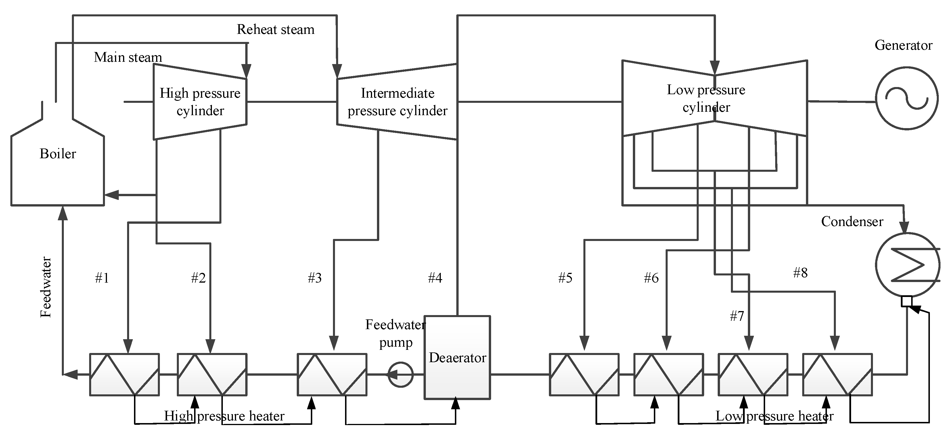
2. Preliminaries and Problems Statement

The research object in the paper is a 600 MW supercritical intermediate reheat condensing steam turbine. The thermodynamic process of this condensing steam turbine can be seen in Figure 1. The feedwater is heated by the boiler and turns into superheated steam. The main steam at a certain pressure and temperature enters the high pressure (HP) cylinder of steam turbine, flows through the nozzle and expands in the nozzle to obtain a high speed. Two extraction stages in HP cylinder feed the #1 and #2 HP heaters. Then, the HP cylinder exhaust goes back into the boiler and then works the reheated steam into the intermediate pressure (IP) cylinder after being reheated. In the IP cylinder, there are two extraction stages supplying the #3 HP heater and the deaerator. Exhaust steam of IP cylinder goes into the low pressure (LP) cylinder with four extraction stages for #5, #6, #7 and #8 LP heaters. The LP cylinder exhaust goes into the condenser as the cold end of Rankine cycle. The heat energy of steam is converted into steam kinetic energy in the nozzle, and the kinetic energy is converted into mechanical energy by the moving blade. The rotors of the steam turbine and generator are connected by coupling. When the rotor of the steam turbine rotates at a certain speed, the generator rotor also rotates, generating electricity.
The heat rate is usually taken as an important index to study and measure the power plant economic performance. Thus, the assessment of the heat rate index has been widely focused on in power plants, and has become one of the important means to monitor the performance of steam turbines [18]. The heat rate value indicates the energy consumed when the turbine generates 1 KWh electricity, calculated as Equation (1)
H R = F g H g F f H f + F r H r F c H c F s p H s p P
where P is the power output; MW: F g , F f , F r , F c and F s p stand for the main steam flow, feed water flow, reheated steam flow, cold reheated steam flow and spray flow respectively; t/h: H g , H f , H r , H c and H s p represent the enthalpy of main steam, feed water, reheat steam, cold reheat steam and spray water, kJ/kg.
Many factors affect the heat rate of the steam turbine unit, and influence the degree that different parameters in the heat rate may be also different. According to Equation (1) and analysis on Rankine cycle, the main steam parameters, reheat steam parameters, feedwater parameters, condenser vacuum and other parameters can be taken as main characteristic parameters for thermal economy analysis in the condensing steam turbine.

3. Methods

Multivariable state estimation technique (MSET) algorithm is a nonlinear multivariate predictive diagnosis technology proposed by Singer [19]. The algorithm is based on the unit’s normal operation data, and estimates the normal operation data under the current condition according to the similarity principle. The actual operation condition of the unit can be judged by comparing the residual between the actual data of the system and the estimated data by MSET algorithm. With the characteristics in dealing with industrial operation data, the MSET algorithm has been widely used in auxiliary equipment fault diagnosis [20] and equipment monitoring [21].

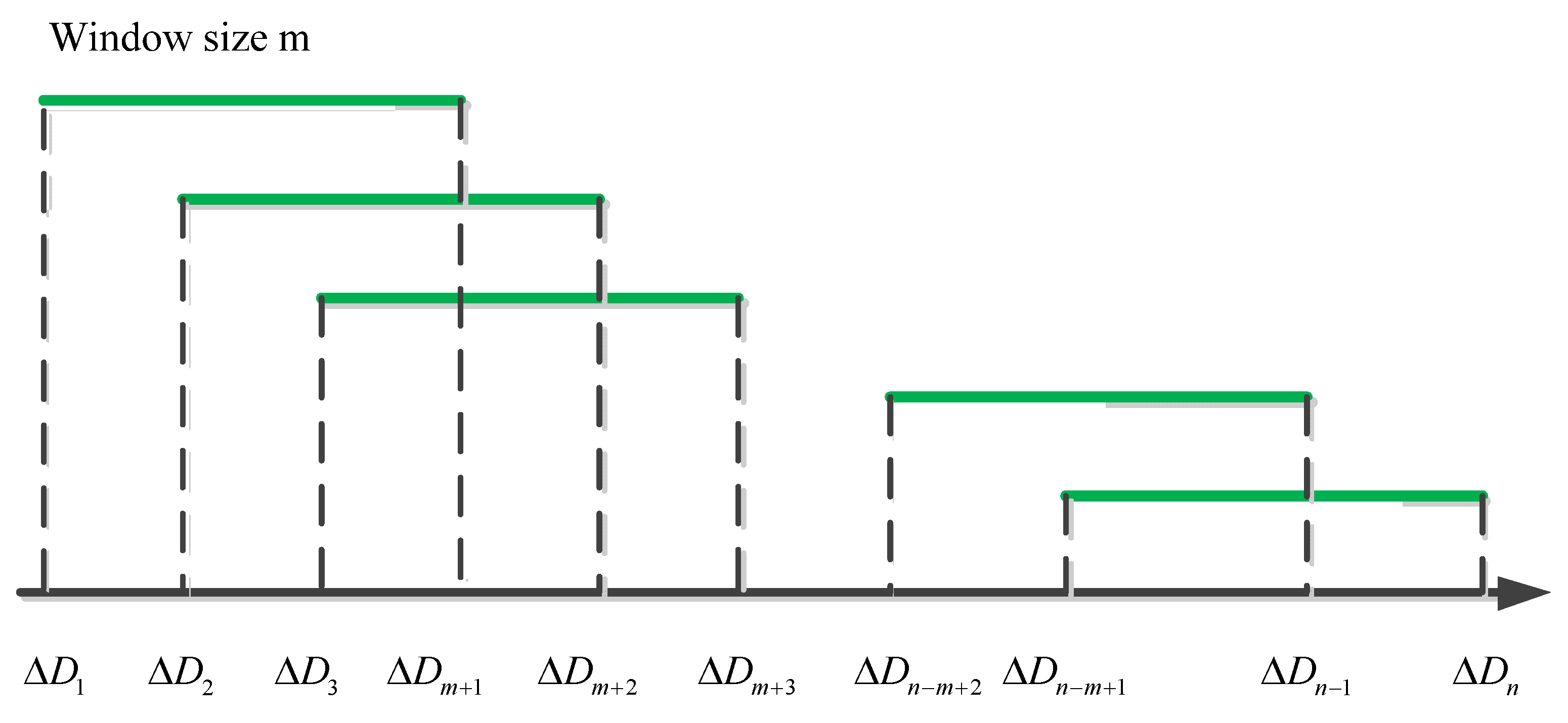
3.1. MSET Method for Parameter Estimation

MSET, a kind of advanced pattern recognition technology, uses the similarity between monitoring parameters under normal operation conditions to realize the state estimation [22]. The algorithm reveals the relationship between parameters based on historical data, and estimates the real state of the object according to the obtained knowledge.
Suppose a system X = [ x 11 , x 12 , , x 1 n x 21 , x 22 , , x 2 n x m 1 , x m 2 , , x m n ] has m data samples and n interrelated parameters. The main steps of MSET algorithm can be listed as follows:
Step 1: Construct memory matrix D , shown in Equation (2). The construction of the memory matrix is the core content of the MSET algorithm, and tends to cover the normal data of all operating conditions, as possible. The purpose to cover the whole normal data is to ensure the accuracy of prediction results. Usually, isometric interpolation method is taken for memory matrix construction.
D = X T = [ x 11 , x 21 , , x m 1 x 12 , x 22 , , x m 2 x 1 n , x 2 n , , x m n ]
Step 2: Calculate estimated vector X e s t according to the actual observed vector X o b s as Equation (3)
X e s t = D · W = D · [ w 1 , w 2 , w m ] T
where W is the corresponding vector weight in D and X e s t is a linear combination of historical observation vectors.
W can be calculated by residual minimization constraint by X o b s and X e s t , as Equation (4)
ε = min | | X o b s X e s t | | = ( X o b s X e s t ) T · ( X o b s X e s t )           = i = 1 n ( X o b s ( i ) j = i m w j D i j ) 2
where ε is the minimum residual value between X o b s and X e s t .
Then, search for the partial derivative of w 1 , w 2 , w m respectively as shown in Equation (5)
( ε ) ( w k ) = 2 i = 1 n ( X o b s ( i ) j = i m w j D i j ) 2 = 0
Convert Equation (5) to be the matrix form as Equation (6)
W = ( D T · D ) 1 · ( D T · X o b s )
Equation (6) can be modified as Equation (7) by using nonlinear operator instead of dot multiplication of matrix, since the matrix D is irreversible.
W = ( D T D ) 1 · ( D T X o b s )
where is a nonlinear operation symbol for Euclidean distance calculation in this paper as Equation (8).
X Y = i = 1 n ( x i y i ) 2
Then, the estimated vector can be obtained by bringing Equation (7) into Equation (3), as the following Equation (9)
X e s t = D · ( D T D ) 1 · ( D T X o b s )

3.2. Modified Information Entropy Weight Method

C. E. Shannon introduced the concept of entropy from the second law of thermodynamics into the field of informatics in 1948, taking entropy to measure the amount of information [23] widely used in various fields. Generally speaking, if the information entropy of a parameter is smaller, it indicates the parameter value has a bigger variation degree. Then, this parameter may contain more information, and can play a more important role in data analysis. On the contrary, a parameter with a larger entropy value means a less important role in index evaluation. Therefore, parameter information entropy values can be calculated to quantize different parameters’ weight in comprehensive evaluation.

3.2.1. Traditional Information Entropy Weight Method

Assume X i j = [ x 11 , x 12 , , x 1 n x 21 , x 22 , , x 2 n x m 1 , x m 2 , , x m n ] as the evaluated object, and X j ( j = 1 , 2 , , n ) as the parameter set. m , n represent data number and parameter number, respectively. The parameter values set { x i j } are then taken to calculate the characteristic weight value set { p i j } as Equation (10).
p i j = x i j i = 1 m x i j
Then, the information entropy value of parameter X j can be expressed as Equation (11)
H j = 1 ln m ( i = 1 m p i j ln p i j )
where ln p i j = 0 when p i j = 0 . 0 H j 1 , and if x i j = x s j , i s , then H j = 1 .
The traditional information entropy weight method uses parameter entropy value for the jth parameter information entropy weight w j 0 calculation as Equation (12) [24]
w j 0 = 1 H j j = 1 n ( 1 H j )
According to Equation (10), the traditional weight values are calculated with the information entropy values listed in Table 1. The information entropy values in four groups are different, seen from Table 1 and Figure 2a. The information entropy difference values by the four groups are 0.0001, 0.001, 0.01 and 0.1, respectively. While the weight values of four groups by the traditional method are the same (0.1667, 0.5000, 0.3333), seen in Figure 2b, w 2 0 w 1 0 = 0.5000 0.1667 = 3 , w 3 0 w 2 0 = 0.3333 0.5000 = 0.6667 . In fact, four groups contain different information deviation, thus, the traditional information entropy weight method leads to an unreasonable result, especially for the small information entropy difference values in groups 1–3 in Table 1.

3.2.2. Modified Information Entropy Weight Method

In order to avoid the shortcomings by traditional information entropy weight method, a weight index w 1 is then calculated as Equation (13)
w j 1 = 1 + H ¯ H j k = 1 , H k 1 n ( 1 + H ¯ H k )
where H ¯ represents the average value of parameters’ information entropy values unequal to 1.
Assume a group of information entropy values as { H j } , including H p and H q . Then, the compound information entropy weight is modified as Equation (14)
w j 2 = { ( 1 H ¯ n ) w j 0 + H ¯ n w j 1 , H j < 1 0 , H j = 1
where the information entropy weight value ratio of H p and H q is then expressed as Equation (15)
w p 2 w q 2 = 1 + H q H p 1 H ¯ 2 + n 1 H ¯ 1 + n H q
The modified information entropy weight method is taken to calculate w 2 2 w 1 2 and w 3 2 w 2 2 with the four group information entropy values as Table 1. The results are shown in Figure 3 with the index n varying from 0 to 50. w 2 2 w 1 2 grows and w 3 2 w 2 2 decreases when n is growing. On the other hand, w 2 2 w 1 2 values with the same n are higher when the information entropy difference values are higher, seen in Figure 3a–c, which is more reasonable than the corresponding results in Figure 2b.
The fourth group in Table 1 shows relatively bigger differences between information entropy values. Thus, curves in Figure 3d can be compared with Figure 2b for the suitable value of n . Table 2 lists w 2 2 w 1 2 and w 3 2 w 2 2 values calculated by the traditional information entropy weight method and the modified information entropy weight method under different n values.
From Table 2, we can see w 2 2 w 1 2 and w 3 2 w 2 2 values tend to be stable when n [ 35 , 42 ] and n can be obtained as 40, compared with w 2 0 w 1 0 and w 3 0 w 2 0 . Thus, the modified information entropy weight method can be clearly expressed as Equation (16)
w j 2 = { ( 1 H ¯ 40 ) w j 0 + H ¯ 40 w j 1 , H j < 1 0 , H j = 1
Therefore, information entropy weight values calculated by Equation (16) can reflect the relationship between information entropy differences and weight values.

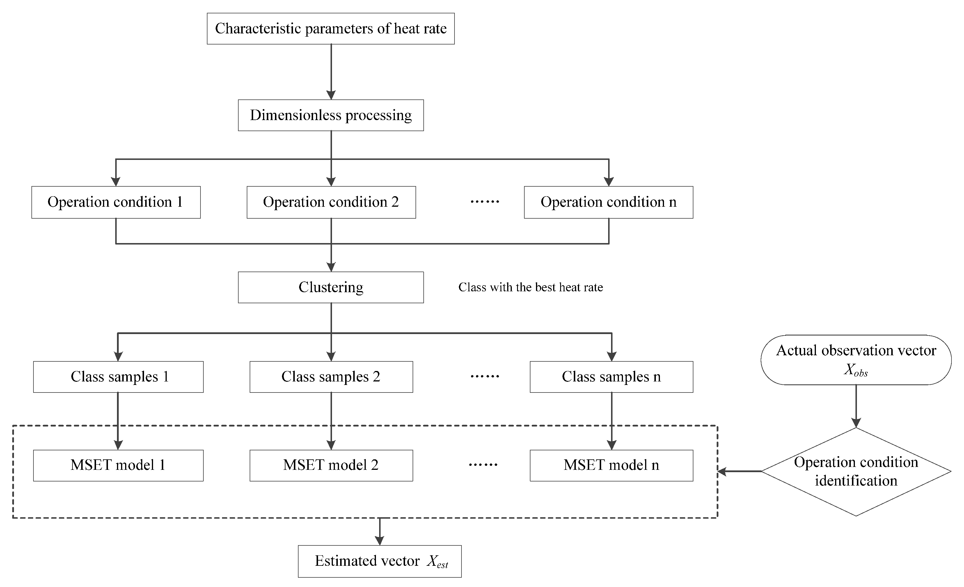
4. Results and Discussion

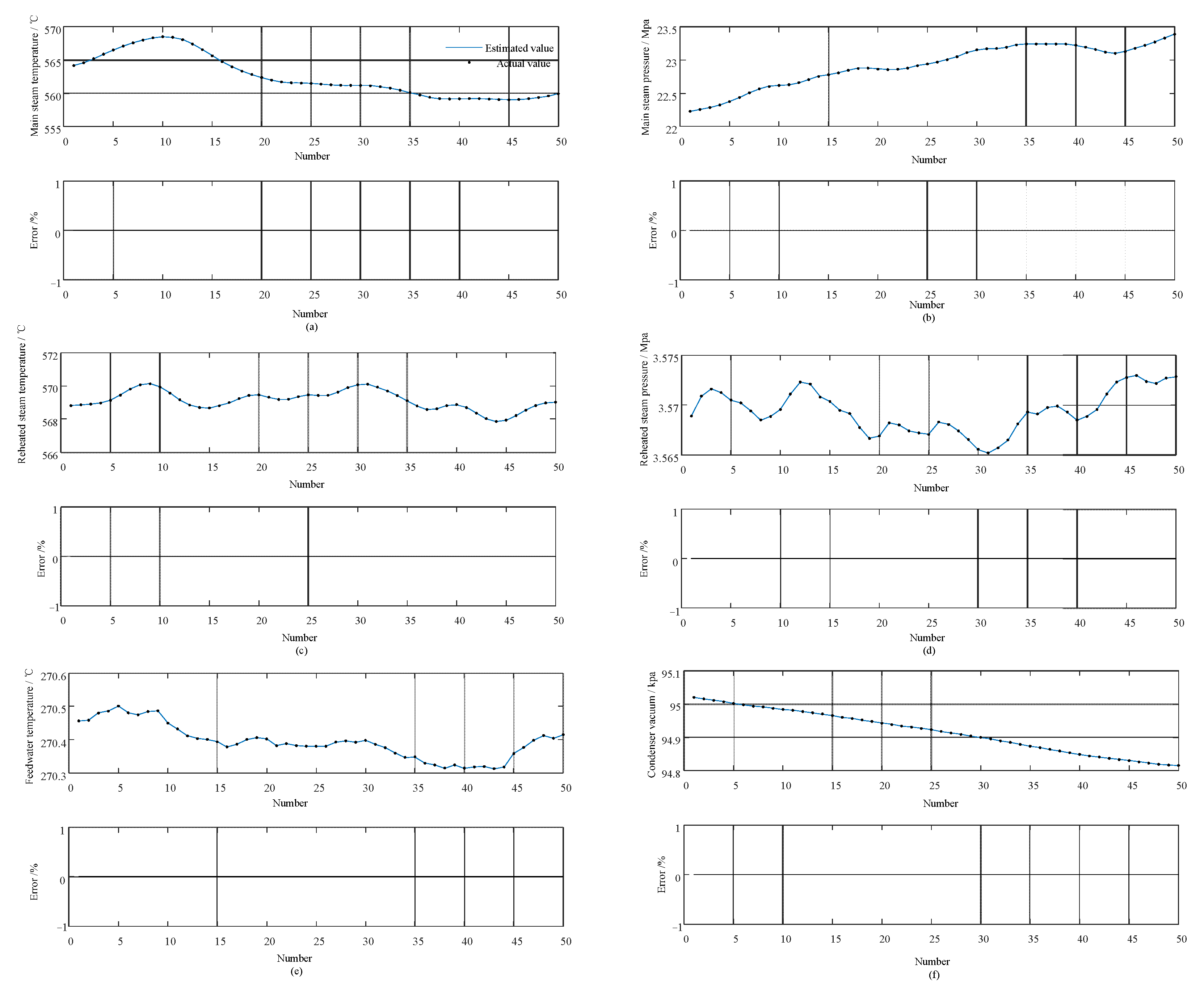
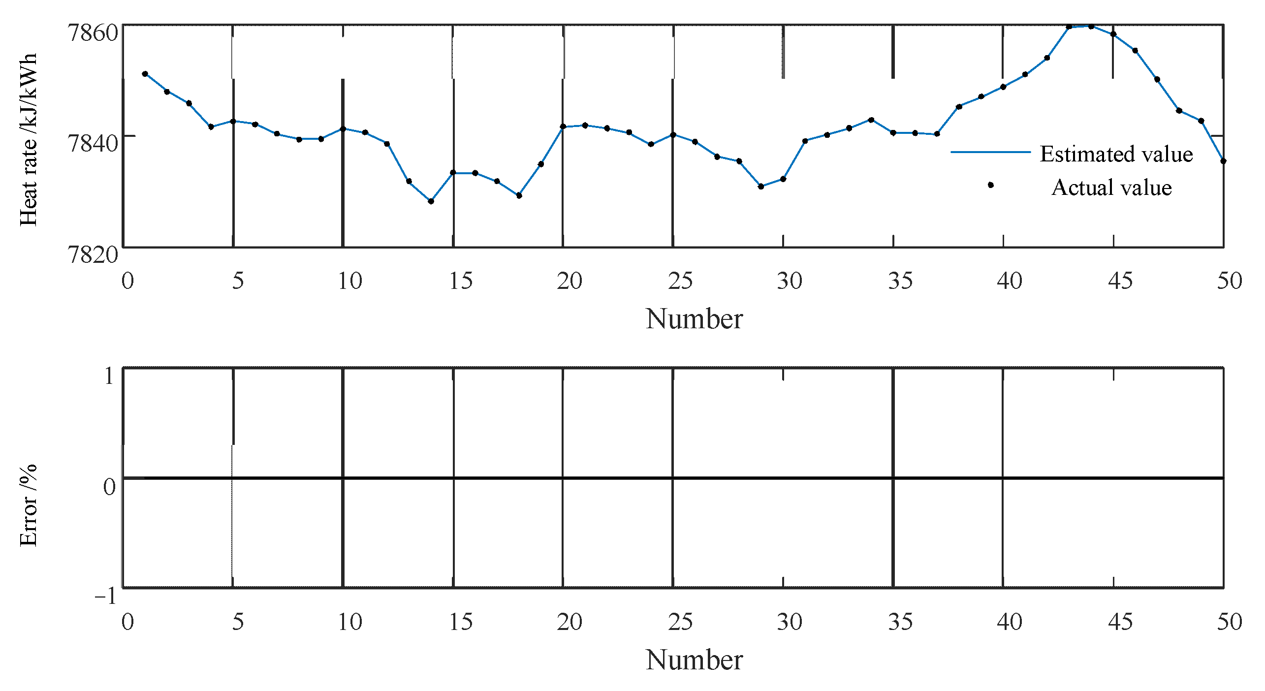
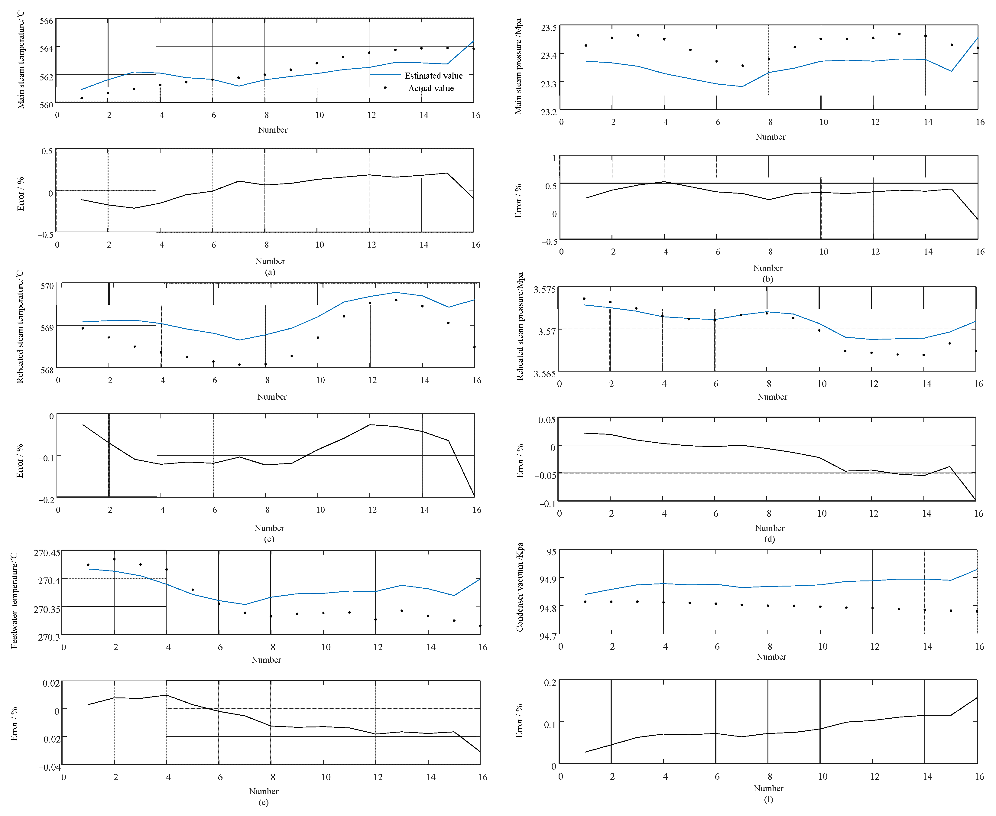
4.1. MSET Model Validation

Energy consumption characteristic data are then selected from steady state database from May 1 to May 30 in 2017, under a 550 MW working condition (with the load in the range (548, 552) MW), and the environment temperature in the range (27, 30) °C. According to Equation (1), unit characteristic parameters of energy consumption containing 13 attributes are seen in Table 3.
After independence and importance analysis, No. 2–7 and No. 13 energy consumption characteristic parameters are respectively selected as condition attributes and decision attribute for clustering under a 550 MW working condition.
The modeling process is shown in Figure 4 for data mining guidance. The 325 data are then clustered by Kmeans method into four clusters, and clustering results based on heat rate can be seen in Table 4. The table shows that #1 cluster contains data samples with the best heat rate, indicating the best working condition. Furthermore, #4 cluster contains those with the highest heat rate, meaning the highest energy consumption, while #2 and #3 clusters are those in the middle level. A total of 50 data from the #1 cluster are then taken as training samples for MSET model, while the remaining 16 data are used to test the established model, seen in Figure 5, Figure 6, Figure 7 and Figure 8.
Figure 5a–f shows the MSET multi parameter estimation model training results of main steam temperature, main steam pressure, reheated steam temperature, reheated steam pressure, feedwater temperature and condenser vacuum. The error percentage values of these energy consumption characteristic parameters are almost equal to zero. Heat rate samples are also trained by the model, with the estimated values, actual values and the error percentage values listed in Figure 6, illustrating a good coincidence degree in the training data. The heat rate values in the figure, calculated with the average value 7839.1 kJ/kWh and the standard deviation value 8.3890 kJ/kWh, indicate the #1 cluster is in a high energy efficiency operation station.
In Figure 7a–f, the MSET multi parameter estimation model is then tested by the remaining 16 samples. The largest error value exists in Figure 7b, displaying the model estimating for main steam pressure with the highest error percentage value of just 0.5%, still small enough for model evaluation. Thus, the error percentage values of these energy consumption characteristic parameters show the accuracy of the MSET model. Heat rate samples are also tested by the model, with the estimated values, actual values and the error percentage values shown in Figure 8. The estimated heat rate values are averaged as 7836.3 kJ/kWh, and with the standard deviation value 2.519 kJ/kWh, while the actual running ones with the average value 7830.1 kJ/kWh and the standard deviation value 4.151 kJ/kWh. The largest error percentage absolute value is 0.24%. The data distribution and error percentage absolute values testify that the MSET model obtains a high accuracy in the #1 cluster.
Moreover, the MSET model established by partial data in cluster #1 is utilized to test the rule between the change in unit operation level and the estimation accuracy. The data from cluster #1, cluster #2, cluster #3 and cluster #4 are taken as test data. Error percentage values are then calculated by parameters as main steam temperature, main steam pressure, reheated steam temperature, reheated steam pressure, feedwater temperature, condenser vacuum and heat rate, seen in Figure 9. Cluster #1 obtains the lowest error percentage values as 0.09%, 0.33%, 0.03%, 0.02%, 0.01%, 0.08% and 0.07%. Further, with the increase in heat rate in cluster #2 to cluster #4, the accuracy of the MSET multi parameter estimation model based on cluster #1 decreases gradually.
Thus, the MSET multi parameter estimation model can be established through the samples in the lowest heat rate group (cluster #1 in the paper), and the residual changes between actual values of the parameters and the estimated ones in the model can be used to monitor unit working condition variation.

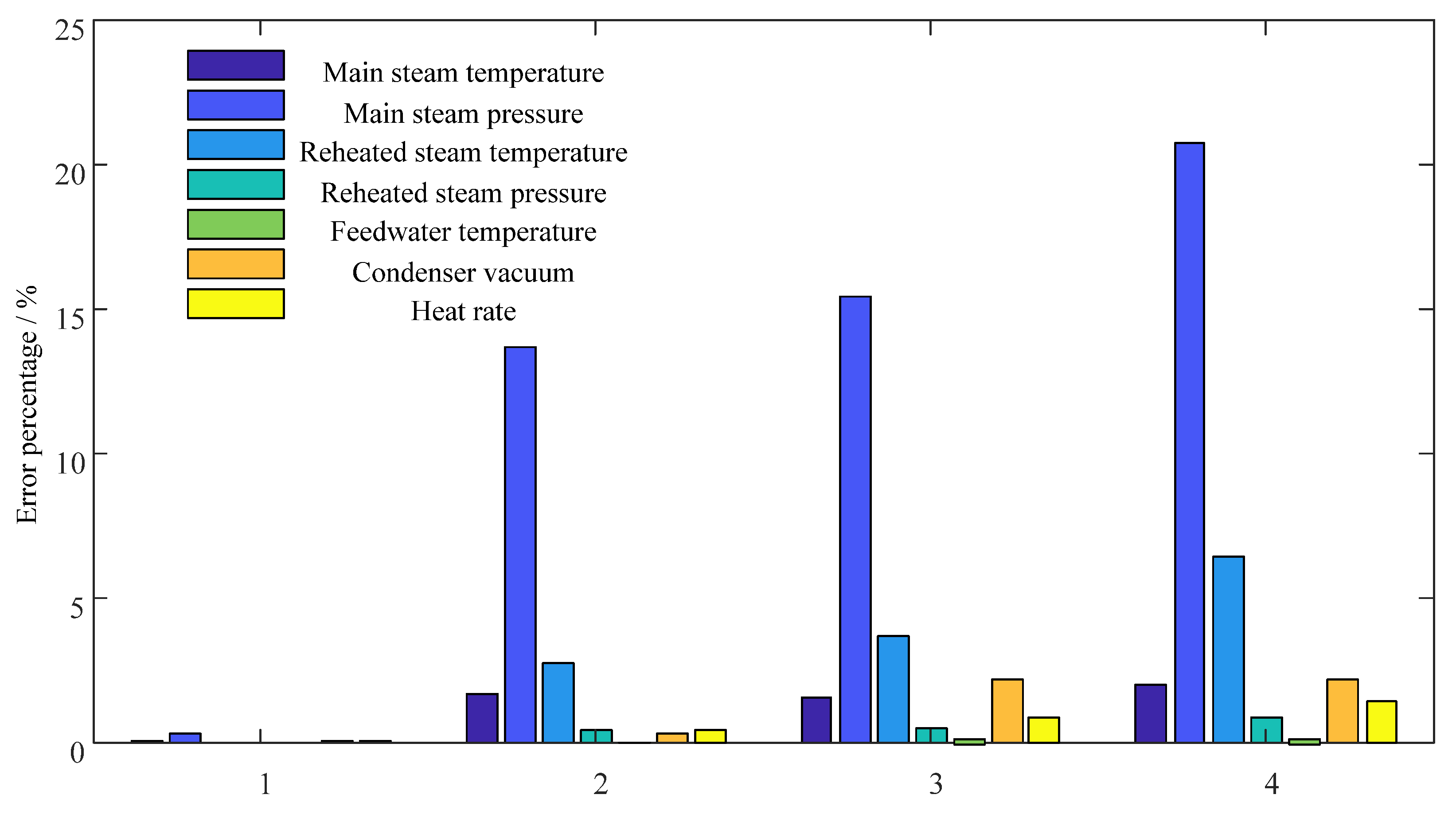
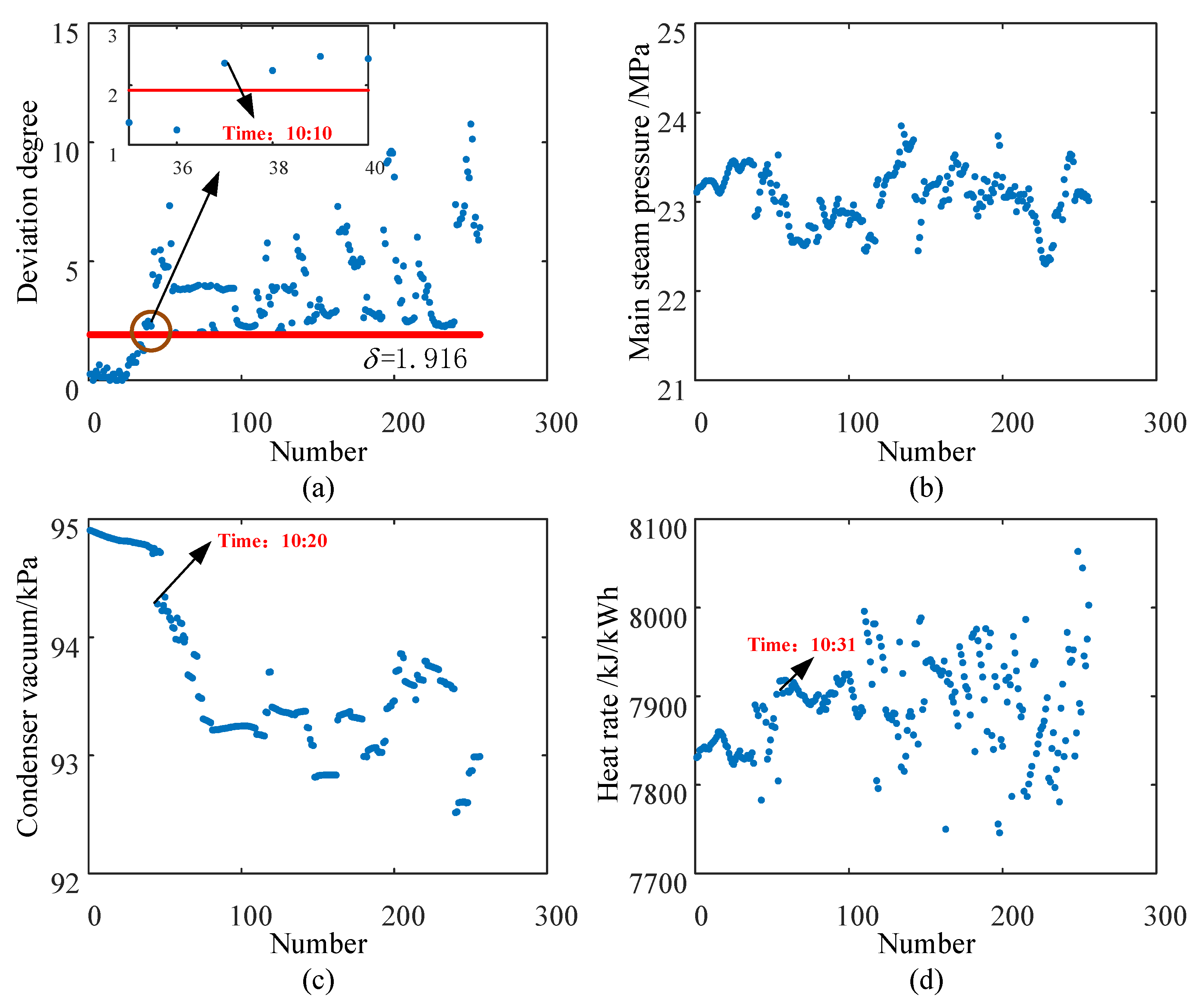
4.2. Case Analysis of Unit Energy Efficiency Monitoring

Unit energy efficiency status can be reflected by differences between actual observed and model estimated values, seen in Section 4.1. Therefore, the deviation degree index calculated by errors of energy consumption characteristic parameters as Equation (17) can measure the energy efficiency.
Δ D i = | X i _ o b s X i _ e s t X i _ o b s | = k = 1 d ( x i k _ o b s x i k _ e s t x i k _ o b s ) 2
where X i _ o b s = [ x i 1 _ o b s , x i 2 _ o b s , , x i d _ o b s ] and X i _ e s t = [ x i 1 _ e s t , x i 2 _ e s t , , x i d _ e s t ] are the actual observed and model estimated values of the ith characteristic parameters, respectively. d is the energy consumption characteristic parameter number. Since parameters have different influences on heat rate, weight values should be added in the deviation degree calculation, as Equation (18).
Δ D i = k = 1 d w k ( x i k _ o b s x i k _ e s t x i k _ o b s ) 2
where w k represents the weight value of kth characteristic parameter, calculated by the modified information entropy weight method in Section 3.2.2.
In Section 4.1, four classes have been clustered by heat rate value with Kmeans method. The deviation degree average value of MSET model with the data from cluster #4 (group with the highest heat rate) as the observation vector can then be taken to determine the energy efficiency warning threshold δ .
Random factors such as measurement errors and noises in the actual operation may lead to a large fluctuation of deviation degree, and even error warnings. Thus, a sliding window method should be used to deal with the deviation calculation.
Assume deviation degree sets Δ D = [ Δ D 1 ,   Δ D 2 ,   ,   Δ D n ] in time sequence, and time window width is m , seen in Figure 10. The ith deviation degree Δ D ¯ i can be calculated as Equation (19).
Δ D ¯ i = 1 m k = i m + 1 i Δ D k
Therefore, the deviation degree index and energy efficiency warning threshold, combined with MSET model under different conditions can be used to handle energy efficiency monitoring in the steam turbine system, and the method’s flow chart can be seen as Figure 11. The steps can be described as follows:
Step 1: based on the heat consumption characteristic parameter condition library, the samples with the highest heat rate under each condition are selected.
Step 2: the energy efficiency deviation warning threshold δ under each condition is determined by the multi parameter estimation model.
Step 3: according to the estimated vector of characteristic parameters under MSET multi parameter estimation model, the deviation degrees of energy efficiency are calculated, and are then processed by the sliding window method for the final deviation degree Δ D ¯ as Equation (19).
Step 4: operation data indicate a normal working condition, unless Δ D ¯ exceeds δ . If Δ D ¯ exceeds δ , there is the necessity for energy efficiency diagnosis and abnormal characteristic parameter location.
Historical data from 2020/05/17 09:34 to 2020/05/17 13:49 with 1 min as the time interval are then taken for the 600 MW steam turbine monitoring, partly listed in Table 5. The environment temperature and power output are (27, 30) °C and (548, 552) MW, respectively.
Characteristic parameters of heat rate in cluster #1 (from Section 4.1) are taken to establish the MSET multi parameter estimation model, and energy efficiency warning threshold δ is 1.916, calculated by data in cluster #4.
The deviation degree values during the period are then shown in Figure 12a, with window width m = 5 . The red line in the figure represents the energy efficiency warning threshold value. The warning happens when the deviation degree value is larger than δ . A partial view is enlarged to clearly tag the 37th deviation degree value, which is the first one larger than δ in the time series. Then, the time stamp of the 37th deviation degree value, 2020/05/17 10:10, is tagged in the figure as the warning time.
Characteristic parameters are then monitored to locate the reason for the abnormal deviation degree values during operation. Figure 12b–d shows the variation of main steam pressure, condenser vacuum and heat rate in time series. In Figure 12b, main steam pressure values cannot be detected, as they contain obvious differences during the period compared with the normal operation data. Other parameters, such as main steam temperature, reheated steam temperature, feedwater temperature and reheated steam pressure have the similar performance. Figure 12c shows that the condenser vacuum suffered a significant decrease at 10:20, 10 min later than the warning time at 10:10. A lower condenser vacuum value indicates a worse working level in the steam turbine system, resulting in a higher heat rate value, seen in Figure 12d. In Figure 12d, the obvious heat rate jump can be caught at 10:31, which is 21 min later than the warning time and 11 min later than the time when the condenser vacuum suffered the significant decrease.
Thus, the heat rate’s abnormal variety in this case can be detected to be caused by the condenser vacuum anomaly. The sudden drop of the condenser vacuum will lead to the decrease in steam energy capacity. In other words, the main steam flow will increase in order to remain at the unit load, which will result in the sudden increase in heat rate value. In this case, the misoperation of valves in the circulating water system causes a sudden decrease in circulating water flow. Thus, a lower condenser vacuum happens when the wet steam into the condenser cannot be sufficiently condensed. When the circulating water system returns to the normal working condition, the heat rate and the deviation degree will gradually fall back.
Actually, many operation parameters influence the heat rate calculation, thus, the time stamp of abnormal heat rate values can be explained later than that of the condenser vacuum in most cases. On the other hand, the heat storage in the boiler can also extend the steam turbine’s heat rate response time when characteristic parameters’ abnormal values exist in operation. Furthermore, while warning time by deviation calculation tagged in Figure 12a is even earlier than the time stamp of the condenser vacuum anomaly, the energy efficiency deviation index can better reflect the change of unit operation state and provide warning information in advance, when combined with the warning threshold δ .

5. Conclusions

In this paper, the MSET model combined with the modified information entropy weight theory is proposed as a method for the steam turbine energy efficiency monitoring study. The parameters’ information entropy average value has been taken into consideration for the modified information entropy weight w 2 calculation, and the modified information entropy weight has been verified to weaken shortcomings brought by the traditional one, w 0 . Then, the MSET estimation model is established by characteristic parameters and the heat rate index under the selected steady 550 MW working condition in a 600 MW unit, with the recognition of the effectiveness in different operation levels being testified. Moreover, the deviation degree index calculated by errors in energy consumption characteristic parameters is proposed to express the current energy efficiency level of the steam turbine. The case study results with data in an abnormal energy efficiency time period show that the method proposed can accurately reflect the change in the unit operation state. Moreover, based on deviation degree values compared with δ , the method proposed in the paper can provide an earlier warning than the time provided by the abnormal heat rate index or energy consumption characteristic parameters. Thus, the combination of the multivariate state estimation technique and modified entropy weight method can be utilized as a new method for field operation guidance.

Author Contributions

Conceptualization, H.G. and H.Z.; methodology, H.G. and H.Z.; validation, H.G., H.Z. and X.C.; investigation, X.C.; data curation, X.C.; writing—original draft preparation, H.G.; writing—review and editing, H.G. and H.Z. All authors have read and agreed to the published version of the manuscript.

Funding

This research was funded by Science Foundation of Nanjing Institute of Technology, grant number CKJA202002.

Data Availability Statement

The data presented in this study are available on request from the corresponding author. The data are not publicly available due to the acquisition from the operation field.

Conflicts of Interest

The authors declare no conflict of interest.

Nomenclature

Abbreviations
mWindow width
pProbability
wWeight value
xData sample
DMemory matrix
FSteam or water flow
HEnthalpy
HRHeat rate of steam turbine
PPower output
WWeight matrix
XData Matrix
Δ D Deviation
Greek symbols
δ Warning threshold
ε Minimum residual value
Superscript
Entropy weight value by traditional method
1Weight index
2Modified weight value calculation
TTransposition
Subscripts
cCold reheated steam
fFeedwater
gMain steam
iThe ith individual
jThe jth individual
mData number
nParameter number
pThe pth enthalpy value
qThe qth enthalpy value
rReheated steam
sThe sth individual
spSpray flow
estEstimated vector
obsObserved vector

References

  1. Ameri, M.; Mokhtari, H.; Bahrami, M. Energy, Exergy, Exergoeconomic and Environmental (4E) Optimization of a Large Steam Power Plant: A Case Study. Iran. J. Sci. Technol. Trans. Mech. Eng. 2016, 40, 11–20. [Google Scholar] [CrossRef]
  2. Luk’yanova, T.S.; Trukhnii, A.D. Studying the effect the parameters of steam power cycle have on the economic efficiency and reliability of three-loop combined-cycle plants with steam reheating. Therm. Eng. 2012, 59, 718–725. [Google Scholar] [CrossRef]
  3. Kumar, M.; Chandra, H.; Banchhor, R.; Arora, A. Integration of Renewable Energy based Trigeneration Cycle: A Review. J. Inst. Eng. India Ser. C 2021, 102, 851–865. [Google Scholar] [CrossRef]
  4. Fu, P.; Wang, N.; Yang, Y.; Xu, H.; Li, X.; Zhang, Y. Tempospacial energy-saving effect-based diagnosis in large coal-fired power units: Energy-saving benchmark state. Sci. China Technol. Sci. 2015, 58, 2025–2037. [Google Scholar] [CrossRef]
  5. Kritskii, V.G.; Berezina, I.G.; Gavrilov, A.V.; Motkova, E.A.; Prokhorov, N.A. Treatment of the Equations of Metal Oxidation Rates at Nuclear Power Plants and Thermal Power Plants in Terms of Thermodynamics. Therm. Eng. 2018, 65, 641–650. [Google Scholar] [CrossRef]
  6. Xu, J.-Q.; Yang, T.; Zhou, K.-Y.; Shi, Y.-F. Malfunction diagnosis method for the thermal system of a power plant based on thermoeconomic analysis. Energy Sources Part. A Recov. Util. Environ. Eff. 2016, 38, 124–132. [Google Scholar] [CrossRef]
  7. Silong, X.; Jianmeng, Y.; Jian, L.; Boshuo, S. Effects of High Pressure Heater Splitting to Heat Economy of Double Reheat Unit. In Proceedings of the 2015 International Power, Electronics and Materials Engineering Conference, Dalian, China, 16–17 May 2015; Atlantis Press: Amsterdam, The Netherlands, 2015; pp. 367–370. [Google Scholar]
  8. Anetor, L.; Osakue, E.E.; Odetunde, C. Thermoeconomic Optimization of a 450 MW Natural Gas Burning Steam Power Plant. Arab. J. Sci. Eng. 2016, 41, 4643–4659. [Google Scholar] [CrossRef]
  9. Shin, J.Y.; Jeon, Y.J.; Maeng, D.J.; Kim, J.S.; Ro, S.T. Analysis of the dynamic characteristics of a combined-cycle power plant. Energy 2002, 27, 1085–1098. [Google Scholar] [CrossRef]
  10. Morini, G.L.; Piva, S. The simulation of transients in thermal plant. Part I: Mathematical model. Appl. Therm. Eng. 2007, 27, 2138–2144. [Google Scholar] [CrossRef]
  11. Nowak, G.; Rusin, A. Using the artificial neural network to control the steam turbine heating process. Appl. Therm. Eng. 2016, 108, 204–210. [Google Scholar] [CrossRef]
  12. Chen, S.; Jiang, Q.; He, Y.; Huang, R.; Li, J.; Li, C.; Liao, J. A BP Neural Network-Based Hierarchical Investment Risk Evaluation Method Considering the Uncertainty and Coupling for the Power Grid. IEEE Access 2020, 8, 110279–110289. [Google Scholar] [CrossRef]
  13. Liu, C.; Niu, P.; Li, G.; You, X.; Ma, Y.; Zhang, W. A Hybrid Heat Rate Forecasting Model Using Optimized LSSVM Based on Improved GSA. Neural Process. Lett. 2016, 45, 299–318. [Google Scholar] [CrossRef]
  14. Fu, Z.; Qi, M.; Jing, Y. Regression Forecast of Main Steam Flow Based on Mean Impact Value and Support Vector Regression. In Proceedings of the 2012 Asia-Pacific Power and Energy Engineering Conference, Shanghai, China, 27–29 March 2012; pp. 1–5. [Google Scholar]
  15. Srinivas, T. Study of a deaerator location in triple-pressure reheat combined power cycle. Energy 2009, 34, 1364–1371. [Google Scholar] [CrossRef]
  16. Qi, M.; Fu, Z.; Chen, F. Research on a feature selection method based on median impact value for modeling in thermal power plants. Appl. Therm. Eng. 2016, 94, 472–477. [Google Scholar] [CrossRef]
  17. Yang, Y.; Li, X.; Yang, Z.; Wei, Q.; Wang, N.; Wang, L. The Application of Cyber Physical System for Thermal Power Plants: Data-Driven Modeling. Energies 2018, 11, 690. [Google Scholar] [CrossRef] [Green Version]
  18. Sun, Y.; Han, X. Research on the Influence of Thermal Performance of Steam Turbine on Energy Loss and Heat Rate. IOP Conf. Series Mater. Sci. Eng. 2019, 677, 032013. [Google Scholar] [CrossRef]
  19. Singer, R.M.; Gross, K.; Herzog, J.; King, R.W.; Wegerich, S. Model-based Nuclear Power Plant Monitoring and Fault Detection: Theoretical Foundations. In Proceedings of the Intelligent System Application to Power Systems Conference, Seoul, Korea, 6–10 July 1997. [Google Scholar]
  20. Tingting, Y.; Yang, B.; Weichun, G.; Huanhuan, L.; Guiping, Z.; You, L. Early Warning Method for Power Station Auxiliary Failure Considering Large-Scale Operating Conditions. In Proceedings of the 2019 IEEE 2nd International Conference on Power and Energy Applications (ICPEA), Singapore, 27–30 April 2019; pp. 11–16. [Google Scholar]
  21. Sun, P.; Jin, G. Research on Satellite Fault Detection Method Based on MSET and SRPRT. In Wireless and Satellite Systems; Wu, Q., Zhao, K., Ding, X., Eds.; Springer International Publishing: Cham, Switzerland, 2021; pp. 33–45. [Google Scholar]
  22. Wang, Z.; Liu, C. Wind turbine condition monitoring based on a novel multivariate state estimation technique. Measurement 2020, 168, 108388. [Google Scholar] [CrossRef]
  23. Xu, W.; Li, M.; Wang, X. Information Fusion Based on Information Entropy in Fuzzy Multi-source Incomplete Information System. Int. J. Fuzzy Syst. 2016, 19, 1200–1216. [Google Scholar] [CrossRef]
  24. Mon, D.-L.; Cheng, C.-H.; Lin, J.-C. Evaluating weapon system using fuzzy analytic hierarchy process based on entropy weight. Fuzzy Sets Syst. 1994, 62, 127–134. [Google Scholar] [CrossRef]
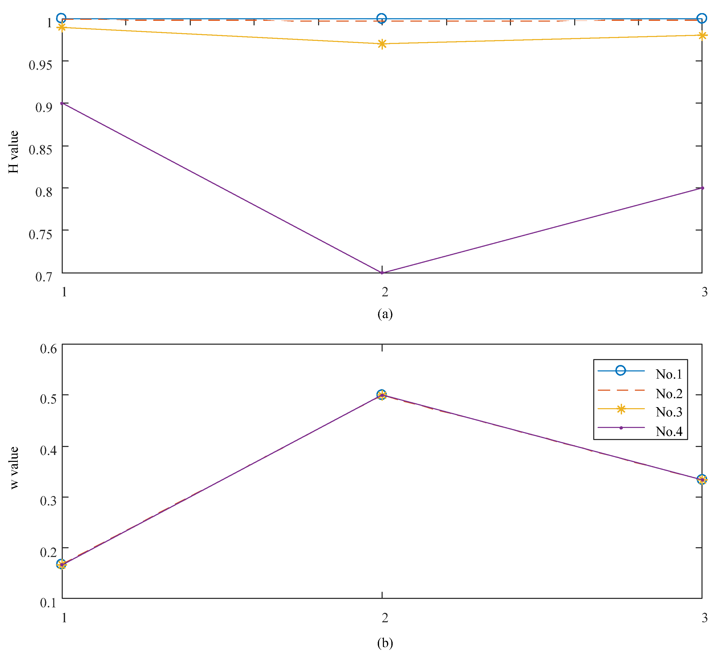
Figure 1. Thermodynamic system diagram of condensing steam turbine.
Energies 14 06795 g001
Figure 2. (a) H values of four sets. (b) Traditional information entropy weight values of four sets.
Energies 14 06795 g002
Figure 3. (a) w 2 2 w 1 2 and w 3 2 w 2 2 varying by different n values in group 1. (b) w 2 2 w 1 2 and w 3 2 w 2 2 varying by different n values in group 2. (c) w 2 2 w 1 2 and w 3 2 w 2 2 varying by different n values in group 3. (d) w 2 2 w 1 2 and w 3 2 w 2 2 varying by different n values in group 4.
Energies 14 06795 g003
Figure 4. The flow chart for establishing heat rate MSET model.
Energies 14 06795 g004
Figure 5. (a) The model training results of main steam temperature. (b) The model training results of main steam pressure. (c) The model training results of reheated steam temperature. (d) The model training results of reheated steam pressure. (e) The model training results of feedwater temperature. (f) The model training results of condenser vacuum.
Energies 14 06795 g005
Figure 6. The model training results of the heat rate index.
Energies 14 06795 g006
Figure 7. (a) The model test results of main steam temperature. (b) The model test results of main steam pressure. (c) The model test results of reheated steam temperature. (d) The model test results of reheated steam pressure. (e) The model test results of feedwater temperature. (f) The model test results of condenser vacuum.
Energies 14 06795 g007
Figure 8. The model test results of the heat rate index.
Energies 14 06795 g008
Figure 9. The error percentage histogram of parameters in four groups.
Energies 14 06795 g009
Figure 10. Deviation degree values in sliding time window.
Energies 14 06795 g010
Figure 11. Flow chart of energy efficiency monitoring method.
Energies 14 06795 g011
Figure 12. (a) Deviation degree values in time series. (b) Main steam pressure variation in time series. (c) Condenser vacuum variation in time series. (d) Heat rate variation in time series.
Energies 14 06795 g012
Table 1. Information entropy values for weight calculation.
NumberEntropy Value
H1H2H3
10.99990.99970.9998
20.9990.9970.998
30.990.970.98
40.90.70.8
Table 2. Weight ratios under different n values.
n3536373839404142
w 2 2 w 1 2 2.99872.99902.99912.99932.99952.99972.99972.9997
w 2 0 w 1 0 3
w 3 2 w 2 2 0.66660.66670.66670.66670.66670.66670.66670.6667
w 3 0 w 2 0 0.6667
Table 3. Characteristic parameters of energy consumption.
No.ParametersUnitAttribute
1LoadMWCondition
2Main steam temperature°CCondition
3Reheated steam temperature°CCondition
4Feedwater temperature°CCondition
5Main steam pressureMpaCondition
6Reheated steam pressureMpaCondition
7Condenser vacuumKpaCondition
8Main steam flowt/hCondition
9Feedwater steam flowt/hCondition
10Condensate flowt/hCondition
11Spray water flowt/hCondition
12Regulating stage pressureMpaCondition
13Heat ratekJ/kWhDecision
Table 4. Clustering results by Kmeans method.
Cluster NumberData NumbersClustering Center of Heat Rate
#1667839.0 kJ/kWh
#21347857.3 kJ/kWh
#3977899.4 kJ/kWh
#4287933.1 kJ/kWh
Table 5. Partial sample data for energy efficiency monitoring.
No.ParametersUnitTime 2020/05/17
9:349:3513:0313:4813:49
1LoadMW550.70550.49551.46548.53550.71
2Main steam temperature°C569.90570.08567.41564.18563.47
3Reheated steam temperature°C561.20561.18563.29558.92558.34
4Feedwater temperature°C270.39270.40270.87271.35271.21
5Main steam pressureMpa23.1123.1523.5124.1223.97
6Reheated steam pressureMpa3.573.573.623.623.64
7Condenser vacuumKpa94.9094.9093.6092.9992.99
8Heat ratekJ/kWh7830.907832.257908.617964.548002.89
Publisher’s Note: MDPI stays neutral with regard to jurisdictional claims in published maps and institutional affiliations.

