Scattering Transform for Classification in Non-Intrusive Load Monitoring

Abstract

Nonintrusive Load Monitoring (NILM) uses computational methods to disaggregate and classify electrical appliances signals. The classification is usually based on the power signatures of the appliances obtained by a feature extractor. State-of-the-art results were obtained extracting NILM features with convolutional neural networks (CNN). However, it depends on the training process with large datasets or data augmentation strategies. In this paper, we propose a feature extraction strategy for NILM using the Scattering Transform (ST). The ST is a convolutional network analogous to CNN. Nevertheless, it does not need a training process in the feature extraction stage, and the filter coefficients are analytically determined (not empirically, like CNN). We perform tests with the proposed method on different publicly available datasets and compare the results with state-of-the-art deep learning-based and traditional approaches (including wavelet transform and V-I representations). The results show that ST classification accuracy is more robust in terms of waveform parameters, such as signal length, sampling frequency, and event location. Besides, ST overcame the state-of-the-art techniques for single and aggregated loads (accuracies above 99% for all evaluated datasets), in different training scenarios with single and aggregated loads, indicating its feasibility in practical NILM scenarios.

1. Introduction

About 60% of the total electrical power generated in the world is consumed by household consumers [1]. Furthermore, in the USA, electricity accounted for 41% of household end-use energy consumption in 2019 [2]. Consequently, electricity consumption habits daily practiced by residential consumers have a significant impact on improving energy efficiency.

Hence, the concept of Load Monitoring emerges. The primary purpose of Load Monitoring is to inform the electrical energy user about the individual appliances energy consumption. With their individual consumption information available, consumers can improve their habits and save energy. There are two general methods to Load Monitoring: Intrusive Load Monitoring (ILM) and Nonintrusive Load Monitoring (NILM).

ILM systems generally correspond to a set of equipment that measures electrical quantities (voltage, current, power, or energy) individually for each appliance and shows those measurements to the consumer. Two fundamental and limiting problems of ILM are the high cost of equipment and the need for adaptation (or intrusion) in the household electrical installation, making its application unfeasible in many cases. On the other hand, a set of computational techniques called NILM, initially presented in [3], was proposed to circumvent such limitations. Those techniques involve pattern recognition, signal processing, and, more recently, deep learning methods. The main idea of NILM systems is to obtain the individual consumption of residential electrical loads from the aggregate energy consumption. In other words, the idea is to determine how the consumption of each device connected to the residential main power line behaves without the need to measure the consumption of each appliance.

Classification and disaggregation of loads are the two main tasks of NILM. The disaggregation determines the load curve for each appliance from the aggregated signal (current, power, or energy). The load classification defines which appliance (or load combination) generated a given load curve. Depending on the framework used, we may have tasks of classification, disaggregation, or both. Comprehensive reviews about NILM are available in [4,5].

NILM techniques can be event-based or nonevent-based. Nonevent-based strategies correlate each section of the aggregated signal with one or more previously known individual load consumption patterns [6]. In the event-based, on the other hand, load transitions are detected, and, subsequently, disaggregation is performed. Generally, NILM classification methods based on events are developed in four basic steps [7]: (i) voltage and current acquisition; (ii) event detection; (iii) extraction of relevant information (features); and (iv) appliance classification.

The feature extraction stage, which is the main focus here, can be applied for high or low-frequency sampling data. High-frequency techniques reveal more discriminative information, as presented in [8] with Voltage-Current (V-I) trajectories, in [9] with current harmonics, in [10] with wavelet coefficients, and [11] with electromagnetic interference.

Recently, state-of-the-art results were achieved for NILM tasks using deep learning-based approaches. The main reasons for that, both in terms of classification and disaggregation, can be summarized as follows: (i) the feature extraction is done automatically through the training process in an end-to-end architecture, without requiring hand-crafted and specifically designed features [12]; (ii) well-known techniques for image processing and CNNs for image classification can be adapted for NILM signals [13]. However, the need for a significant amount of training data and the high computational cost spent on training convolution filters are challenges yet to be overcome [14].

Thus, we can highlight the following research gaps regarding the application of convolutional networks for NILM:

• CNN-based methods depends on trained filter coefficients, which raises the overall classification system complexity;
• Most part of the methods using CNN for NILM takes advantage of image-processing CNN approaches. These approaches use 2D data as input, which also raises the system overall complexity, once it is necessary to transform the original 1D electrical signal to a higher dimensional 2D data;
• As CNN filter coefficients are learned, large datasets are desirable, causing a data availability dependency problem.

In this context, S. Mallat [15] proposed a time-frequency representation called Scattering Transform. In this transform, a time series (1D data) is converted to the time-frequency domain employing a cascade association of convolutions with wavelets, followed by the modulus operator. Thus, the Scattering Transform (ST) has an architecture similar to the CNN, as analytically detailed in [16]. This transformation proved to be robust for classifying different image [17] and audio [18] tasks. The ST does not require data augmentation techniques or datasets with a relatively high number of instances to obtain state-of-the-art results, since its coefficients are previously calculated instead of fully learned as observed in CNNs.

To cover the cited above research gaps, we intend to answer the following question [19]: is it possible to reach equivalent or better classification results than state-of-the-art techniques for NILM with a nontrained convolutional network? Hence, we can formulate the following objectives [19]:

• Disaggregate and classify NILM signals from publicity datasets with a novel ST-Based framework;
• Evaluate classification performance and compare it with state-of-the art techniques;
• Encourage future work to replace CNN with ST in the context of NILM;
• Encourage future smart meter real-time implementations, with a less computationally costly NILM classification method.

To meet the set of objectives, by taking advantage of the features extracted from the ST, we propose a framework for classifying aggregated electrical load signals in the NILM context. To the extent of our knowledge, this work is the first to use the ST in the NILM context to face the related research gaps. In the proposed framework, we first preprocess data from public datasets, and then apply the ST to the preprocessed samples. We apply a strategy to extract features from the ST output signals, leading to appliances signatures based on ST. After that, we split training and testing subsets and use machine learning classification models to predict the classes (loads). In the end, we calculate accuracy and FScore as performance indicators.

We compare our results with state-of-the-art methods, considering two publicly available high-frequency datasets: LIT-Synthetic [20] and PLAID [21]. Among the main advantages of the proposed method, especially when compared to deep learning techniques, we can highlight:

• The quality of the extracted features, obtaining superior results in terms of accuracy and FScore for most analyzed cases;
• No need for data augmentation, transfer learning techniques, or dataset composition to increase the classification accuracy.

The remainder of this paper is organized as follows. Section 2 demonstrates the main gaps of related works and the contributions and originality of this research. Section 3 presents in detail the datasets, preprocessing, feature extraction, and classification strategy. Section 4 details the results for different experiments. We discuss the results and compare them with related work in Section 5. Finally, Section 6 shows the conclusions, practical implications, limitations, and suggestions for future works.

2. Related Work

The CNN-based classification and disaggregation methods applied to NILM are organized, in this section, by the sampling frequency of the dataset. We discuss the low-sampling-frequency methods (i.e., less than 3 Hz) first, and in the sequence, high-frequency approaches.

2.1. CNN for NILM Using Low-Frequency Data

Several works use low-frequency datasets to train CNN architectures for disaggregation or NILM classification [1,22,23,24,25,26]. In [22], for instance, the authors proposed a sequence-to-sequence 1D-CNN architecture for NILM with superior disaggregation results for high-power loads, but with an inability to disaggregate low power loads. Similarly, in [23], a low-frequency load disaggregation architecture called CAEBN-HC was proposed, which is a 1D-CNN with batch normalization (BN) and hill climbing (HC). The authors extracted the temporal features with a CNN, applying BN to avoid explosion or vanishing gradient in the training process. HC was applied to adjust the hyperparameters, and the results obtained were promising, i.e., from 7 to 10W of Mean Absolute Error (MAE). However, the authors only addressed the disaggregation of few loads with high power, and did not present results in terms of low power and several aggregated loads. Chen et al. [23] explain in the conclusions section the intention to use data augmentation to improve the results with more aggregated loads. In [1], the authors proposed a deep CNN architecture for NILM classification, with accuracy results greater than 96% for the REDD dataset. Moradzadeh et al. [1] proposed to classify appliances of households not included in the training stage, but the disaggregated load curves were not available, and the results are limited to only three selected loads.

The SCANnet proposed in [24] used Context-Aware Feature Integration, which is a map of additional features used to learn the contextual information for NILM disaggregation. The disaggregation results, MAE in the range of 9–16 W, were comparatively superior to the literature but limited to only six electrical loads with relatively high power, and dependent on data augmentation with Wasserstein GAN. The work proposed in [25] presented a CNN architecture called TP-NILM for load classification. The authors used electrical power as an input signal for the CNN. The feature extraction technique only detected whether the appliance is active and what was its average consumption in that mode. A stage called temporal pooling, which aggregates the features of different resolutions, was added in [25], which improved the temporal context. Both disaggregation and classification were performed in [25]. The accuracy results were up to 97% for seen classes and up to 78% for previously unseen ones. The approach discussed in [25], on the other hand, is based on a multilabel strategy to classify multiple loads in the UK-DALE dataset. However, only three electrical appliances were simultaneously analyzed. A Multi-Channel Recurrent Tapped Delay Line CNN network (MR-TDLCNN) was proposed in [26], with training and testing in the AMPds dataset. The authors used three input channels on a CNN for disaggregation: active, reactive, and current power. This approach increased the discriminability, and the MAE results varied between 4.8–18 W. The drawback was the need for more input data w.r.t. the other compared methods due to the architecture’s overall size.

In [27], the authors applied a spatial clustering using density-based for applications with noise to classify different load curves. The idea of combining expert knowledge and deep learning models led up to 95% accuracy, overcoming other state-of-the-art deep learning methods. However, the method in [27] needed a multifeature method to transform the 1D load data into 2D matrix data. Authors in [28] proposed a 2D CNN structure that recognizes the load status. The proposed method used Gramian angular fields (GAFs) for encoding appliance low-frequency power series (1D) to an image (2D). The authors produced their own dataset and, consequently, proper comparisons are hampered.

The CNN-LSTM hybrid model proposed in [29] overcame CNN and LSTM methods for UK-DALE dataset in terms of accuracy (up to 98.87%). Despite these good results, the proposed CNN-LSTM method presented a much longer test time than CNN and LSTM ($1031\mathsf{\mu }$s vs. $23\mathsf{\mu }$s and $27\mathsf{\mu }$s respectively). Furthermore, CNN-LSTM needed a large amount of data for training to avoid overfitting, besides the performance depended on the depth of the neural network. D. Ding et al. [30] proposed a disaggregation method independent of the depth of the CNN. The proposed method was based on multiple overlapping sliding windows that avoid overfitting and gradient vanishing in NILM. Authors in [30] introduced a new extension of CNN called inception structured CNN to deal with NILM. FScore results (up to 70.7%) and the accuracy (up to 76.7%) overcame other deep learning methods when considering different sliding windows, but the proposed structure is complex and has a large set of trained filters. A comprehensive up-to-date review of deep models applied to low-frequency NILM can be found in [31].

2.2. CNN for NILM Using High-Frequency Data

Although low-sampling-frequency data are easily obtained directly from smart meters, the extracted features are not as discriminative as those obtained with high-frequency datasets [32]. Discriminative features for low power consumption appliances or transient features for devices containing switched static converters, for instance, cannot be achieved with low-frequency methods. In this section, we present methods that use data with high-sampling-frequency to overcome those limitations.

In several classification and disaggregation methods, a 2D image is generated from the one-dimensional NILM signal, allowing the use of well-known image processing and deep learning techniques for NILM classification. In [33], the 2D image was generated by a time-frequency Short-Time Fourier Transform (STFT). The spectrogram was applied as the input of a CNN, particularly designed for that work. The good location both in time and frequency allowed to deal with non-stationary multi-component signals, but some classification accuracy results were below the average of other methods, i.e., around 70% for the PLAID dataset. A similar approach is presented in [34], in which spectrograms obtained from an STFT were used as input of the CNN. The strategy was devised to filter out background noise caused by other loads in the target load. In [35], the 2D representation was weighted pixelated V-I images, obtained from the normalized V-I curve in steady-state. The image was then inserted as the entry of a CNN, which performs the classification. The overall FScore was also below the average of the other compared methods (<78%), and the authors needed to use 2 datasets together (PLAID and WHITED) to reach those results.

Two multilabel approaches were presented in [6,13]. Both have the advantages of being multilabel classification strategies, presented as alternative approaches to the traditional 2D image applied to the input of a CNN. In [13], a transition event is first located, followed by the Fryze Power Theory in the aggregated current to extract the features together with a similarity matrix based on the Euclidean distance to reinforce the discriminability. A 2D image is then generated, being the input of a CNN with multilabel classification. In [6], on the other hand, a multilabel approach was proposed to improve the classification of loads of the same type but different brands. Given one cycle of the voltage and current, a Weighted Recurrent Graph (WRG) generates a 2D image for posterior classification. Accuracy results were better than other baseline methods that produce 2D images from V-I trajectories, but still lower than those presented in [13] (both for PLAID dataset). Moreover, results of [6] were obtained from submetered data (i.e., not aggregated).

Accuracy results above 98% were obtained in [14], which presented a technique called 2D phase encoding (2DPEP) to generate a 2D image from the NILM signal. However, the proposed approach used other classification methods based on classical machine learning, increasing the complexity. In [12], a discrete wavelet transform to obtain a 2D image from the aggregated current signal is proposed. The authors used the image as an input to a sequence-to-sequence CNN. The wavelet transform has the advantage of time-warping stability, but the data used in [12] were submetered, and not naturally aggregated. The same limitation is found in [12,36]. Particularly in [36], the authors employed a deep convolutional autoencoder to extract features from individual hospital loads. Nevertheless, there is no disaggregation since the CNN input is obtained from a submetering network. In [7], a multiagent strategy was proposed to improve NILM classification, achieving accuracy results above $95\%$ on LIT-dataset. Although this result was superior to the related literature, applying the multiagent strategy in realistic cases may be compromised due to the high computational complexity. The authors in [37] also presented a CNN-based classification model for NILM, reaching $92\%$ global accuracy on LIT-dataset, but with limitations in the feature extraction for loads with similar transitory shapes.

A real-time CNN-based method proposed in [38] reached up to 99.2% accuracy, with a 100 Hz sampling frequency data. This method uses a three-stage structure: (i) event detection; (ii) CNN classification; and (iii) power estimation, applying machine learning to detect the turn-on events and an heuristic algorithm to estimate the real time power. However, there were some limitations, such as: (i) authors used a private dataset, which reduces reproducibility; (ii) only three appliances of greater power consumption were used in the tests; (iii) the algorithm had problems in identifying loads with steep step-up transients.

2.3. Contributions and Originality of This Work

Based on the criteria exposed so far, one can observe that the related works have several positive aspects and some limitations, such as: (i) reliance on large sets of training data, and strategies such as data augmentation, multichannel input networks, or associating more than one dataset for training may be necessary to achieve higher accuracies; (ii) in CNN, convolution filters are generally learned and not calculated analytically, which requires higher computational costs and, consequently, a more considerable amount of data; (iii) the classification strategies with CNN for NILM, that use time-frequency features available in the literature, usually apply 2D data (images) as input from the convolutional network, and not directly the 1D data sequence from the electrical loads, which may compromise the feature extraction. Considering those limitations, the main contributions of this paper are:

• A NILM classification framework using a convolutional-based network with the scattering transform, without the need to learn filter coefficients to extract features, reducing the amount of data required in the training process;
• An approach with better classification performance compared to the state-of-the-art methods for different publicly available datasets (LIT and PLAID);
• A time-frequency feature extraction technique that directly uses 1D data as input, reducing the overall complexity and increasing the class discriminability.

3. Proposed Classification Strategy

To present all the sets of results and comparisons with related works, two different approaches were employed. The feature extraction, the classifiers’ training, and evaluation for the test set were carried out with the same dataset in the first approach, which is the most conventional analysis [32]. In the second approach, the feature extraction and the training were conducted in one dataset, and the prediction was evaluated in a different dataset. In this second case, we train models with single and three loads and evaluate the model’s classification performance with two, three, and eight loads. Therefore, it is possible to analyze the classifier’s generalization, as proposed in [7]. Figure 1 shows the two approaches, detailed as follows.

3.1. Lit Syntetic Dataset

The first dataset used in this work is the LIT Synthetic (LIT-SYN) [20]. This is a subset of the full LIT-Dataset and it refers to acquisitions collected from a bench, in which real loads are connected, but the network loads’ switching instant is controlled. This set contains 1664 waveform acquisitions sampled at 15,360 Hz, with precisely annotated (<5 ms) switching events of 26 classes (loads). The aggregated AC grid voltage and current acquisitions are monitored for periods of up to 40 s. The devices used in this subset are summarized in

Table 1. Appliances in LIT Synthetic Subset (LIT-SYN).

ID	Device	Rated Power (W)
1	Microwave Standby	4.5
2	LED Lamp	6
3	CRT Monitor	10
4	LED Panel	13
5	Fume Extractor	23
6	LED Monitor	26
7	Cell phone charger Asus	38
8	Soldering station	40
9	Cell phone charger Motorola	-
10	Laptop Lenovo	70
11	Fan	80
12	Resistor	80
13	Laptop Vaio	90
14	Incandescent Lamp	100
15	Drill Speed. 1	165
16	Drill Speed. 2	350
17	Oil heater power 1	520
18	Oil heater power 2	750
19	Microwave On	950
20	Air heater Nilko	1120
21	Hair dryer Eleganza—Speed 1	365
22	Hair dryer Eleganza—Speed 2	500
23	Hair dryer Super 4.0—Speed 1—Heater 1	660
24	Hair dryer Super 4.0—Speed 1—Heater 2	1120
25	Hair dryer Parlux—Speed 1—Heater 1	660
26	Hair dryer Parlux—Speed. 2—Heater 1	885

.

LIT-SYN contains different subsets with different multiple aggregated loads, starting with isolated loads (LIT-SYN-1), two combined loads (LIT-SYN-2), three (LIT-SYN-3), and eight (LIT-SYN-8). The authors of the dataset also make available a subset with all combinations, defined as LIT-SYN-Total.

3.2. Plaid Dataset

The second subset is the Plug-Load Appliance Identification Dataset (PLAID), proposed in [21]. It is a high-frequency (30 kHz) public dataset, and it has submetered data for 17 electrical appliances, totaling 1876 measurements in 65 different homes. PLAID also has a subset of aggregated data, composed of 1314 waveforms of 13 electrical appliances (classes) present in a test laboratory, which is used here. The aggregated measurements are obtained in combinations of two or three electrical loads, with annotations of connection and disconnection events for each load.

Table 2. Appliances in aggregated subset PLAID.

ID	Device	Rated Power (W)
1	Compact Fluorescent Lamp	13
2	Fridge	Not available
3	Fridge Defroster	Not available
4	Air Conditioner	740
5	Laptop	Not available
6	Vacuum Cleaner	Not available
7	Fan	38
8	Incandescent Light Bulb	100
9	Blender	Not available
10	Coffee Maker	975
11	Water Kettle	1500
12	Hair Iron	Not available
13	Iron Solder	60

shows the set of aggregated electrical loads from the PLAID dataset. We use the aggregate subset of measurements in this work.

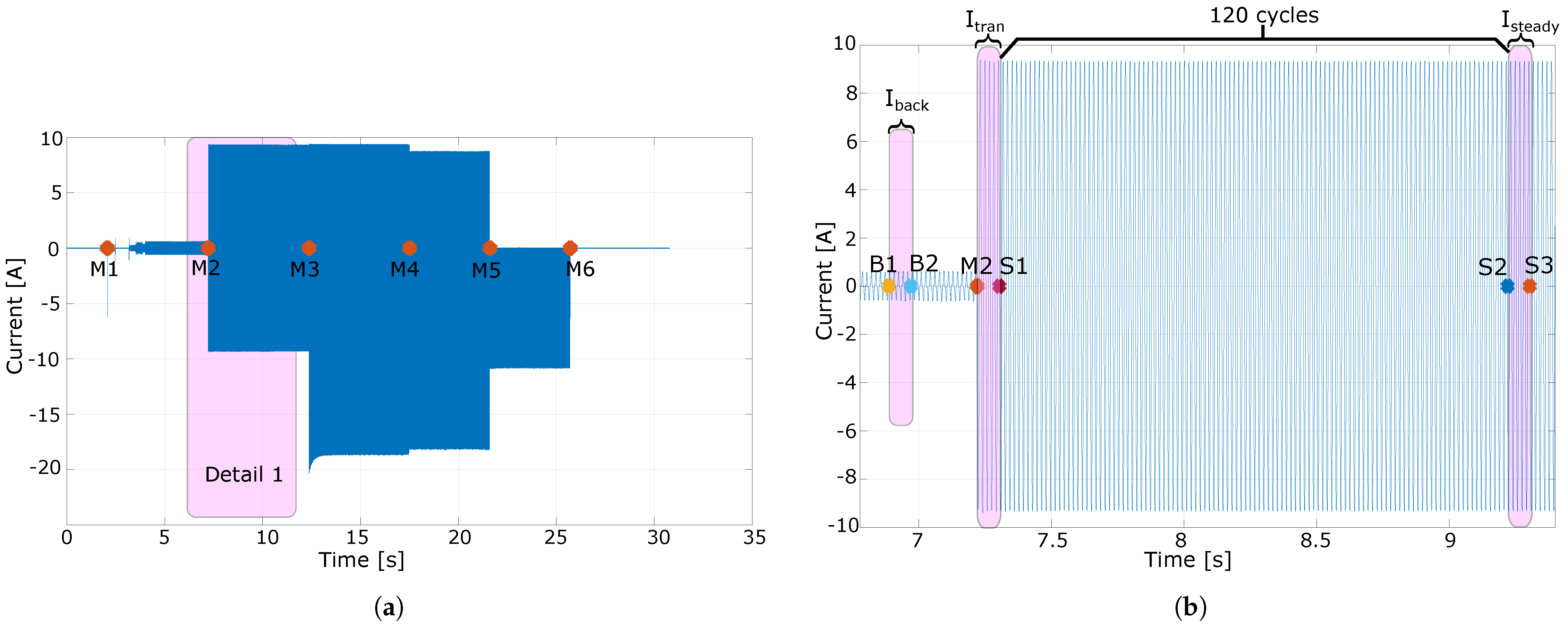
3.3. Preprocessing and Disaggregation

For the preprocessing and disaggregation, different scenarios are considered, as summarized in

Table 3. Experimental scenarios description.

Scenario	${\mathit{n}}_{\mathbf{back}}$	${\mathit{n}}_{\mathbf{cycles}}$	Selected Region	${\mathit{n}}_{\mathbf{feat}}$
A	30	20	SS + T	118
B	30	20	T	59
C	30	20	SS	59
D	20	5	SS + T	86
E	20	5	T	43
F	20	10	SS + T	102
G	20	10	T	51
H	20	10	SS	51
I	40	40	SS + T	134
J	40	40	T	67
K	40	40	SS	67

. Each chosen scenario has one particular time region of the electrical NILM signal, detailed as follows.

The selected regions may be in Steady State (SS), Transient (T), or both states. Scenarios A, D, F, and I consider SS and T regions by concatenating the energy coefficients from those regions. Scenarios B, E, G, and J consider only transient instants. Scenarios C, H, and K consider steady-state regions. Each scenario assesses a different number of cycles, $n_{back}$, before the turn-on event, considered for the disaggregation procedure. With those scenarios, the authors intend to verify the robustness of the proposed feature extraction strategy for variations applied to the ST input signals. The region selected for each scenario has ${\mathrm{n}}_{\mathrm{cycles}}$ cycles of the aggregated signal. The ${\mathrm{n}}_{\mathrm{feat}}$ is detailed in Section 3.4.

To exemplify, we present how we construct Scenario D and E. In Figure 2a, the first three red markers (M1–M3) indicate the turn-on events for a sample extracted from the LIT-SYN-3 subset. The last three red markers (M4–M6) indicate the turn-off events. Firstly, our algorithm defines a point (B1), with $n_{\mathrm{back}}=20$ cycles before M2. Then, we take a window ($I_{\mathrm{back}}$) from B1 to B2, with $n_{\mathrm{cycles}}=5$ cycles. In the sequence, we compute two signal windows after M2. The first is the transient current region ($I_{\mathrm{tran}}$), and the other is the steady-state current window ($I_{\mathrm{steady}}$). The $I_{\mathrm{tran}}$ is between the first zero-crossing after M2 and $n_{\mathrm{cycles}}=5$ after its zero-crossing, reaching S1. The $I_{\mathrm{steady}}$ is located between 120 cycles after P1 (point S2) and S3, that is located $n_{\mathrm{cycles}}=5$ cycles after S2. The windows $I_{\mathrm{steady}}$ and $I_{\mathrm{tran}}$ are then used to compute the disaggregated data, $I_{\mathrm{tran}}^d$ and $I_{\mathrm{steady}}^d$. As in [8], the transient and steady-state disaggregated data are defined as $I_{\mathrm{tran}}^d=I_{\mathrm{tran}}-I_{\mathrm{back}}$ and $I_{\mathrm{steady}}^d=I_{\mathrm{steady}}-I_{\mathrm{back}}$, respectively. For Scenario D, we concatenate both signal windows $I_{\mathrm{tran}}^d$ and $I_{\mathrm{steady}}$. For Scenario E, we directly apply the feature extraction on $I_{\mathrm{tran}}^d$.

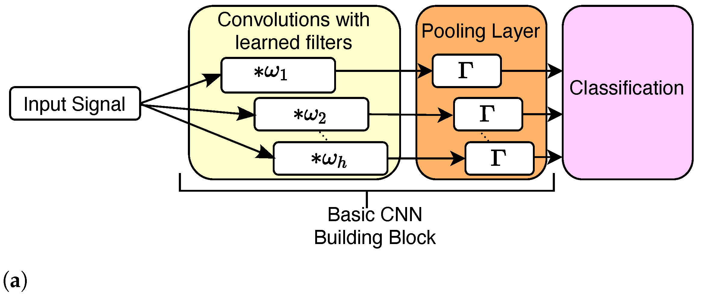
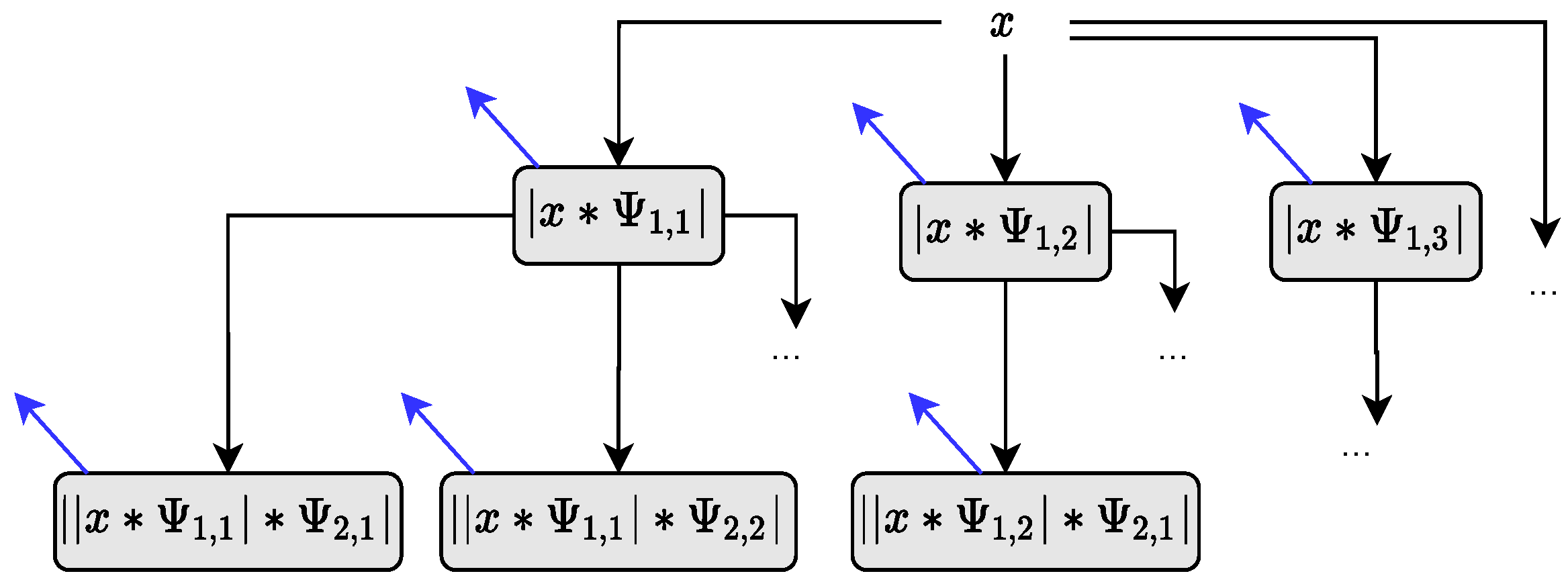
3.4. Feature Extraction

Before presenting the proposed feature extraction with the ST, we first explain here the structural differences between classical CNN and ST. The typical structure of a CNN comprises, as shown in Figure 3a, an input layer followed by one or more stages of activation, convolutional, and pooling layers (subsampling) [39]. The discrete convolution operation applied in each feature extraction stage takes an input signal $x\left[k\right],k\in \mathbb{N}$ and results [40] in the sequence $s_h\left[k\right]$, given by:

$$s_h\left[k\right]=\sum _{a=-\infty }^{\infty }x\left[a\right]{\omega }_h[k-a]=x\left[k\right]\ast {\omega }_h\left[k\right].$$

(1)

The sequence ${\omega }_h\left[k\right]$ contains the convolutional filters (or kernels) coefficients for the h-$th$ convolutional filter of the related feature extraction stage. These filter coefficients are generally learned in the training process [39,40]. The pooling stage, on the other hand, applies the nonlinear operator $\mathsf{\Gamma }$ to $s_h\left[k\right]$ (typically ${\mathsf{\Gamma }}_h$ is the maximum value or average value), and decreases the dimension of $s_h\left[k\right]$.

The Scattering Transform consists of convoluting an input signal with a set of wavelets [15], and then applying modulus and average operator to the convolutional stage output. Figure 3b represents the average operator by ${\mathsf{\Phi }}_T$.

The Discrete Wavelet Transform (DWT), the core of ST, maps a 1D signal $x\left(t\right)$ into a 2D array of coefficients [41], such that:

$$x\left(t\right)=\sum _{k=-\infty }^{\infty }{c}_k\phi (t-k)+\sum _{k=-\infty }^{\infty }\sum _{j=0}^{\infty }{d}_{j,k}\psi (2^{j}t-k),$$

(2)

in which $\phi \left(t\right)$ is the scaling function, $\psi \left(t\right)$ is the mother wavelet, $c_k$ is the k-th scaling coefficient, and $d_{j,k}$ is the detail coefficient for the scale j and the discrete time k. The mother wavelet is translated by k and scaled by j, and this gives both ST and DWT good localization in time and in frequency domains [41]. The multiresolution filter banks approach is suitable for computational implementation of DWT [41].

Unlike CNN, the ST convolutional layer filters, represented by ${\mathsf{\Psi }}_n,n\in [1:h]$, in Figure 3b are already predetermined by wavelets [41], and therefore there is no need for training. Besides that, both CNN and ST structures have nonlinearity layers. In Figure 3a, CNN presents a pooling layer, and in Figure 3b, ST has a modulus and an average layer. The modulus and the average provides to ST the stability to small time-warpings and local time-shifting invariance properties, but there is a loss of information [15]. To recover that, the modulus layer output must be convoluted with a new set of wavelet filters, at a different scale [15]. These properties are detailed as follows.

Consider two NILM signals from the same appliance: $x\left(t\right)$ and a time-warped signal $x_{\tau }\left(t\right)=x\left(t\right)-\tau \left(t\right)$, where $\tau \left(t\right)$ is a non-Gaussian small deformation. In the real world, these deformations can occur when considering two brands of the same appliance [42]. We want a feature extractor that is stable to these small variations.

Additionally, consider the time-shifted signal $x_c\left(t\right)=x\left(t\right)-c$, being c a constant. In NILM applications, these cases can happen when the same electrical load is turned on at different times within a defined interval. A feature extractor with invariance to such time-shifting is desirable since it can decrease dependence on event detectors.

Wavelet transforms [41] are stable to small time-warpings, but covariant with time-shifting. To deal with this limitation, the authors in [15] introduced the Scattering Transform. This transform consists of complex wavelet transform applied successively to the input signal, cascading with the contractive modulus operator [43] and average. Considering that the maximum order is m and the maximum scale is J, for the layer $q<m$, the coefficients of ST are given by:

$$S_q\left(x\right)={\left|\left|\left|x\ast {\mathsf{\Psi }}_{j_1}\right|\cdots \ast \right.{\mathsf{\Psi }}_{j_q}\right|\ast {\mathsf{\Phi }}_J}_{j_1<\cdots <j_q<J},$$

(3)

where ${\mathsf{\Psi }}_{j_k}$, $k\in [1:q]$ is a wavelet function and ${\mathsf{\Phi }}_J$ is a low-pass filter. The scattering coefficients of $x\left(t\right)$ are aggregated in a set $S_J$, given by:

$$S_J\left(x\right)={\left\{S_q\left(x\right)\right\}}_{0\le q\le m}.$$

(4)

The modulus gives to the ST the time-shifting invariance property, and the cascaded convolutions with ${\mathsf{\Psi }}_{j_k}$, ($1\le k\le q$) recovers the high-frequency information lost with the modulus-average operations [15,42,44]. The implementation in discrete time is performed with filter banks [41].

When applied to a 1D signal x, the ST distributes the energy of x across paths and layers. The first layer performs a convolution between x and a complex Gabor wavelet. The result is the input of the second layer, causing each path to be a multiresolution convolutional network. This process imposes the information to be dispersed in different orders and paths in a convolutional architecture [43].

The first-order coefficients, $S_1$, are obtained by convoluting the signal x with the wavelet ${\mathsf{\Psi }}_{j_1}$, which is a complex bandpass filter. Then, the modulus operator is applied to the result. To guarantee stability [44], the first-order coefficients are obtained by convolution of the module with a low-pass filter ${\mathsf{\Phi }}_J$, and then $S_1=\left|x\ast {\mathsf{\Psi }}_{j1}\right|\ast {\mathsf{\Phi }}_J$.

The structure of the convolutional network that implements the Scattering transform is shown in Figure 4. In our case, the electrical signal x passes through the first layer of convolutions with the wavelets ${\mathsf{\Psi }}_{m,j}={\mathsf{\Psi }}_{1,j_1}$. The subscript $j_1$ is the frequency scale of the first filter bank. The convolution modulus is taken at each node of the tree in the first layer. The output of each node in the first layer is used to calculate the second level of the convolutional network. At the second level, the output of nodes of type $\left|x\ast {\mathsf{\Psi }}_{1,j_1}\right|$ is convoluted with a second set of wavelets, of the type ${\mathsf{\Psi }}_{m,j}={\mathsf{\Psi }}_{2,j_2}$. The $j_2$ index represents the second frequency scale of the transform ($m=2$), implemented by the second filter bank. Each second layer node is obtained by taking the convolution modulus with ${\mathsf{\Psi }}_{2,j_2}$.

The blue arrows in Figure 4 represent the convolution operation with the low-pass filter ${\mathsf{\Phi }}_T$. The cutoff frequency of ${\mathsf{\Phi }}_T$ is half the bandwidth on the j scale. The features used for classification are the results of those convolutions, represented by the blue arrows in the Figure 4.

We use the Wavelet Scattering library, from Matlab^® R2021a to implement the ST. We consider different scenarios for the extraction and selection of features from the ST of the electrical signal. The number of features (${\mathrm{n}}_{\mathrm{feats}}$) for each scenario is the number of wavelets filters (J) for the first layer of Scattering Transform (order 1). This number depends on the quality factors of the first-order filter bank (Q) and the total number of samples for each input signal (T). We computed the approximated number of Scattering Coefficients ($n_j^k$), resulting of j-th wavelet filter convolution for the scenario $k\in \{A,B,\cdots ,K\}$, through Algorithm 1.

Algorithm 1 Number of scattering coefficients.

Input:Q and probability parameter ($PP$). Output:$n_j^k$    1: for each scenario k ∈ $\{A,B,\cdots ,K\}$ do    2:   Compute T, the number of samples per examples.    3:   Compute $cv$, the Gaussian critical value for the probability parameter $PP$, as detailed in [45].    4:   Compute ${\sigma }_{\mathsf{\Phi }}^f=\frac{T}{2\times cv}$, the frequency standard deviation for the scaling function.    5:   Compute the frequency support for the scaling function (${\mathsf{\Phi }}_{support}$), as discussed in [15].    6:   Compute the highest wavelet center frequency ${\omega }_{\mathsf{\Psi }}=\frac{2\pi }{1+2^{\frac{1}{Q}}}$.    7:   Compute the frequency standard deviation for the wavelets ${\sigma }_{\mathsf{\Psi }}^f={\omega }_{\mathsf{\Psi }}\frac{1-2^{-\frac{1}{Q}}}{1+2^{-\frac{1}{Q}}}\frac{1}{\sqrt{\frac{3}{10}ln\left(10\right)}}$.    8:   $J\leftarrow \mathrm{floor}\left\{Q\left[lo{g}_2\left({\sigma }_{\mathsf{\Psi }}^f\right)-lo{g}_2\left({\sigma }_{\mathsf{\Phi }}^f\right)\right]\right\}$.    9:   Compute ${\mathsf{\Psi }}_{tsupport}^f$, the time support of the j-th first layer wavelet filter.  10:   $\mathrm{res}\leftarrow \min \left[lo{g}_2\left(\frac{2\pi }{{\mathsf{\Psi }}_{tsupport}^f}\right),0\right]$.  11:   $n_j^k\leftarrow \mathrm{round}\left[\frac{T}{2^{\mathrm{res}}}\right]$.  12:   return$n_j^k$  13: end for

Feature Calculation from Scattering Coefficients

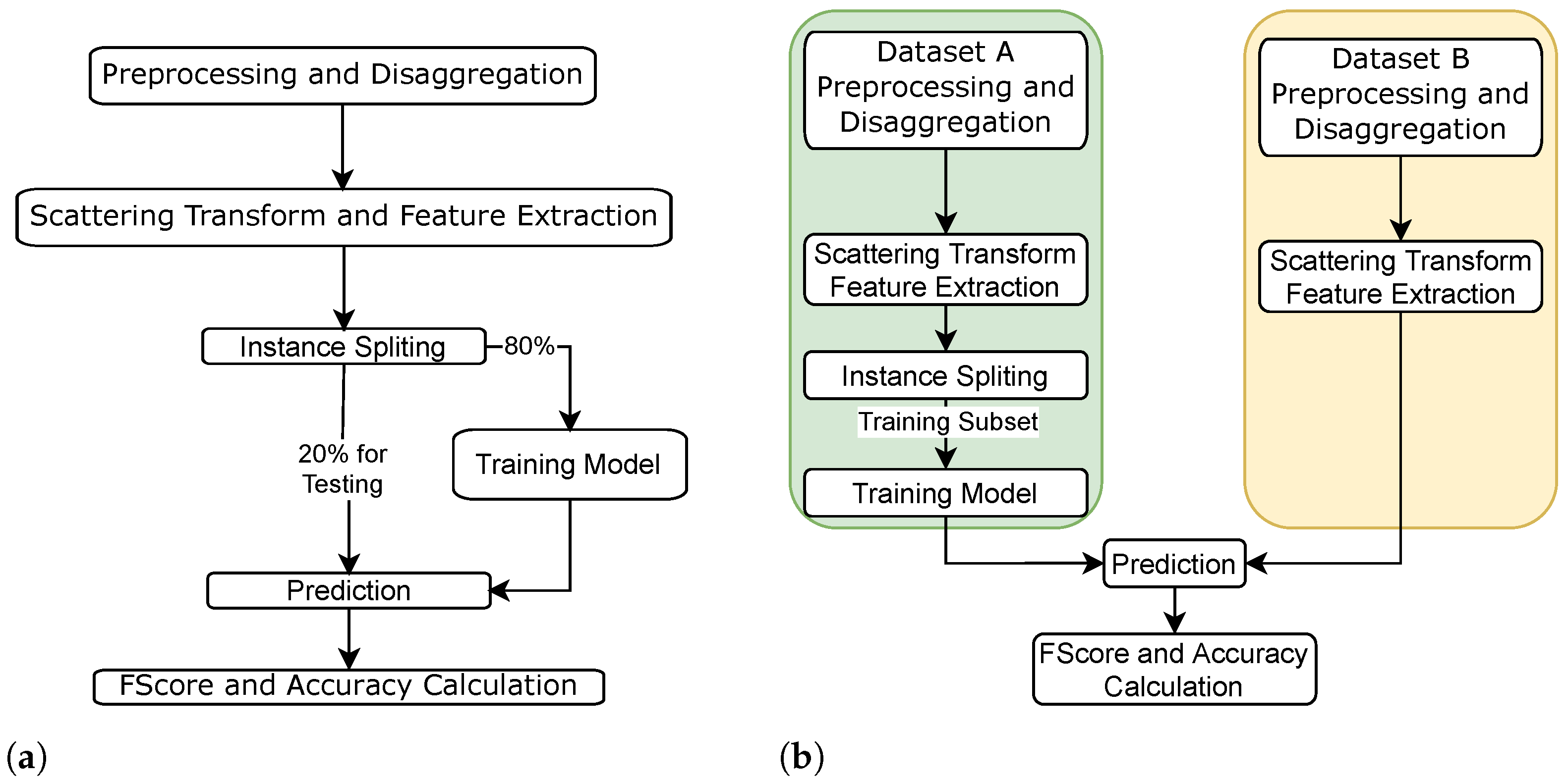
Let $\left\{S_{1,j}\right\}$ be the set of first-order scattering coefficients determined by the j-th wavelet filter. Then, we propose the energy calculation for the j-th feature, $f_j$, as:

$$f_j=\sum _{p=1}^{n_j^k}{S}_{1,j}{\left[p\right]}^2,$$

(5)

with $\mathbf{f}\in {\mathbb{R}}^{{\mathrm{n}}_{\mathrm{feat}}\times 1}$, indicating the number of features per scenario presented in Table 3. Finally, both rigid translation and time-warping variabilities in the NILM signals need to be mitigated to represent the signals. The invariance to translation is desirable to NILM signals as the event detection is not always accurate or available. Both Deep CNN and ST have these properties, but in the case of ST: (i) it is possible to optimize filters and pooling nonlinearities; (ii) the multiple layers are analytically determined; and (iii) there is no training stage for the filters coefficients [42].

3.5. Classification

The electrical appliance classification task follows the steps described in Figure 1a,b. The training and test sets are separated from the feature matrix and the vector of labels. From the complete matrix, 80% of the instances were used to train the classifier and select parameters using five-fold cross-validation. For testing, the remaining 20% were evaluated. All the features are normalized in $[-1,1]$.

We train five different classification methods, typically used in NILM approaches [7]: K-Nearest Neighbors (k-NN), Ensemble Method (ENS), Support Vector Machines (SVMs), Decision Trees (DTs), and Linear Discriminant Analysis (LDA), briefly detailed as follows:

• k-Nearest-Neighbors: this method classifies the test example by comparing it to the training dataset. The comparison is based on the Euclidean distance [46]. This method fully relies on the distances between test samples and the training set, and due to that, can be considered one of the simplest classification approaches [46]. However, it requires the storage of all training examples, which may be a limitation for embedded systems with more restrictive memory requirements [7].
• Decision Tree: this method employs several concatenated binary splits arranged in a tree structure. Each split (node of the tree) refers to a particular feature and the corresponding parameter value for the comparison. In the test stage, the example is evaluated at each node of the tree and the corresponding class is the majority class in the leaf node. The training process and the related splits are based on the information gain [46].
• Support Vector Machine: this classifier was proposed to maximize the separation margin between pairs of classes, based on a linear model (hyperplane) [47]. One of the great advantages of the SVM formulation is that it can be formulated as a convex optimization. Besides, the problem can be defined in terms of the dot product between the features. Therefore, by using the kernel trick, the dot product can be replaced by a dot product kernel in feature space using the kernel, allowing nonlinear separation between classes [46]. Here, we used the Gaussian kernel to evaluate nonlinear separations.
• Ensemble Method: this method combines different weak learner models by averaging the output of individual classifiers, improving the final accuracy [46]. Weak models usually have a poor individual response in terms of accuracy. However, combining the various classifiers tends to improve overall accuracy. One example is the random forest method that combines several decision trees to compose a final classification. The ensemble normally uses the following weak models: AdaBoostM1, AdaBoostM2, Bag, GentleBoost, LogitBoost, LPBoost, LSBoost, RobustBoost, RUSBoost, Subspace, and TotalBoost [46].
• Linear Discriminant Analysis: The LDA is a linear classifier that employs hyperplanes to differentiate data from two different classes. It assumes a normal distribution with an equal covariance matrix and equal priors for both classes. With that, the separating hyperplane is defined by reducing the dimensionality in such a way that it maximizes the separation between classes and minimizes the intraclass variance. So, its complexity, and consequently, overfitting, are reduced [46].

4. Results

Initially, in Section 4.1, we perform the two approaches presented in Figure 1. In the first approach, the experiments consider the same subsets of LIT-SYN for training and testing. Subsequently, as shown in Figure 1b, the experiments are conducted varying the number of loads for training and testing (different subsets), aiming at evaluating different scenarios and generalizations for the model. Since the PLAID dataset does not contain subsets with a different number of aggregated loads, in Section 4.2, we present only the results for the approach presented in Figure 1a. For all the experiments in Section 4.1 and Section 4.2, we include other two baseline methods for comparisons: (i) V-I trajectory [8] and (ii) Discrete Wavelet Transform (DWT) [48]. Those methods are selected since they are part of the state-of-the-art results presented in [7] and both extract transient and steady-state features, allowing direct comparisons for all experimental scenarios described in Table 3. In Section 5, a discussion and a comparison with deep learning-based and state-of-the-art results for LIT-SYN and PLAID is shown to present further the positive aspects of the ST feature extraction and classification.

4.1. Lit-Syn Dataset

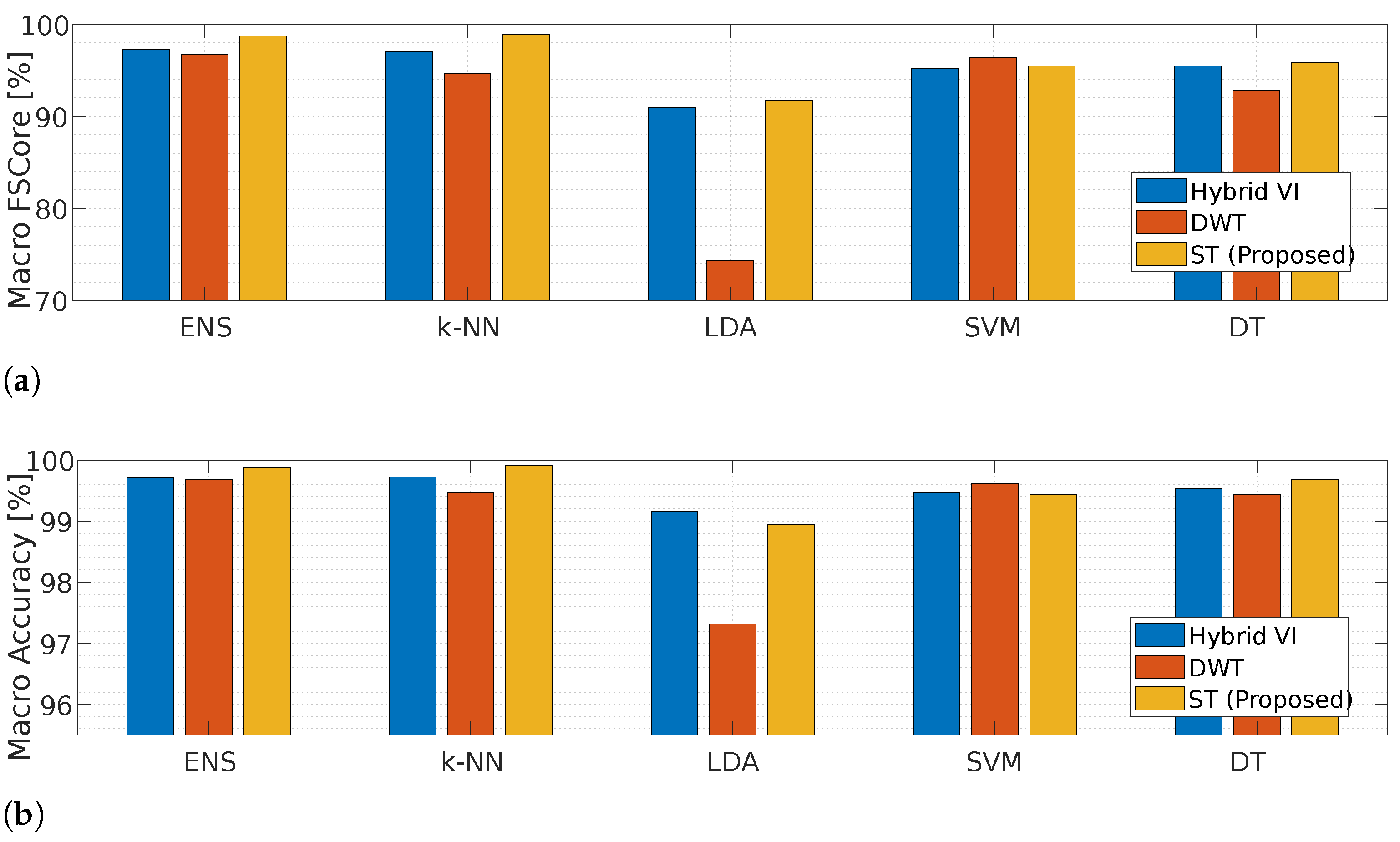
4.1.1. Results Using the Same Subset for Training and Testing

We performed the strategy proposed in Figure 1a, training the five classification models for each scenario of Table 3. We show in Figure 5 the comparison of the macro FScores and Accuracies among the proposed method and the baseline methods. The results were obtained as follows: (i) for each scenario and each LIT-SYN subset, we obtained the average of the five-fold macro FScore and Accuracy for five classification models; (ii) for each LIT-SYN subset, we choose the best scenario results for each classifier; and (iii) we performed the averages of the best macro FScores and Accuracies among the LIT-SYN subsets.

From Figure 5, we can conclude that the proposed method presented better performances than baseline methods for ENS, k-NN, and DTs. Additionally, ST reaches the two highest macro FScore and Accuracy averages, with 98.74% (FScore) and 99.87% (Accuracy) for ENS, and 98.93% (FScore) and 99.91% (Accuracy) for k-NN.

Based on the results for the best classifier (ENS), for each subset of the LIT dataset, and considering all the scenarios of Table 3, we calculated the average macro FScore and Accuracy. The results are shown in Figure 6.

To verify the influence of the scenarios presented in Table 3, Figure 7 shows macro accuracies and FScores for the LIT-SYN-8.

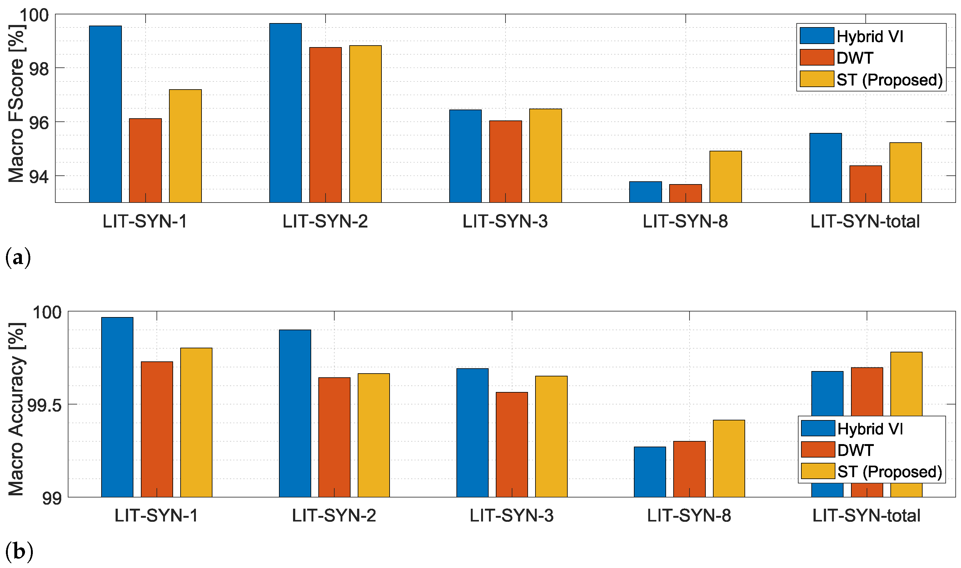
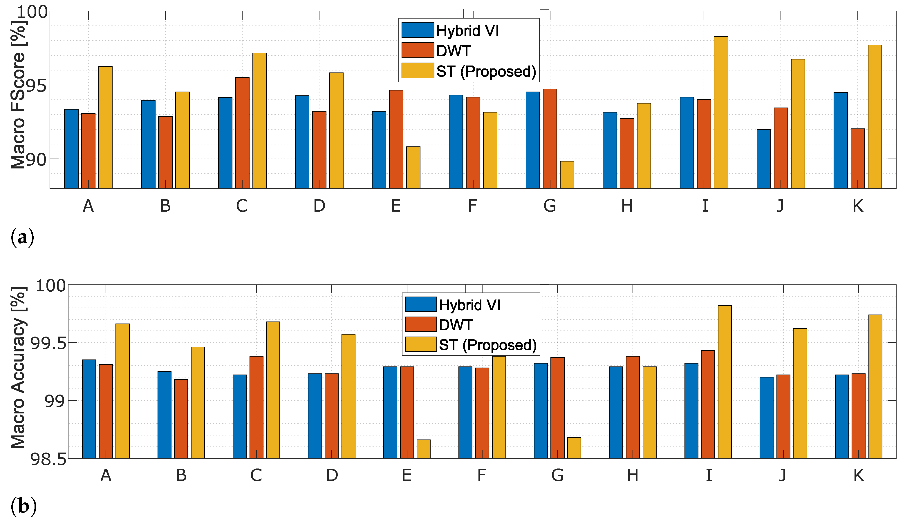
4.1.2. Results Using Different Subsets for Training and Testing

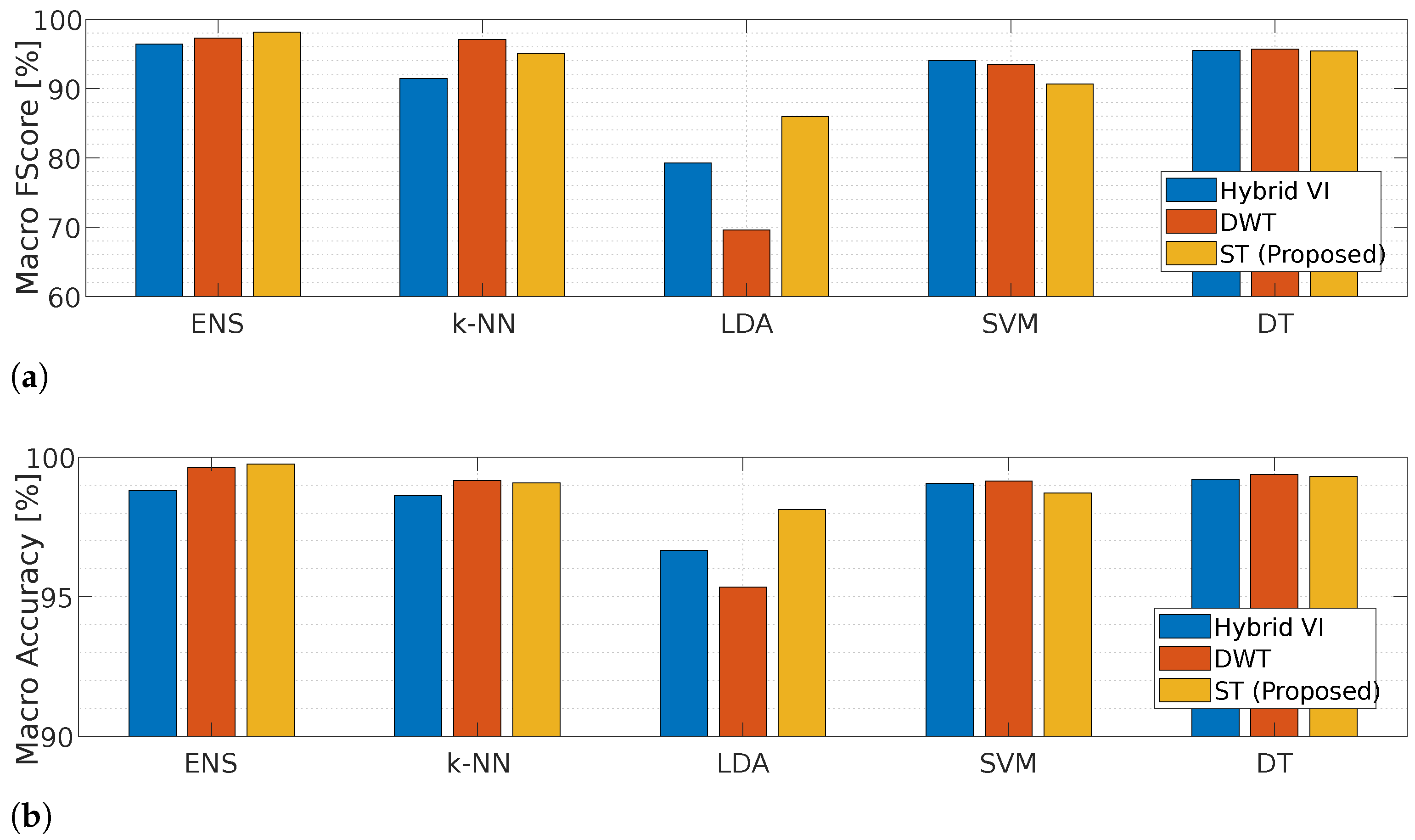
As presented in [7], the actual scenario of data collection in NILM systems may involve the acquisition of single or multiple loads, depending on the availability and difficulty in acquiring samples. Hence, to verify in terms of classification accuracy how much the typical signature of an electric load is maintained as multiple loads are added, we present the generalization analysis in this subsection.

We first extract features with ST considering the best accuracy and FScore performance previously obtained with the same subsets for training and testing. For comparison purposes, classification models are also trained using the V-I and DWT methods for the same training and test subsets, with the best classifiers for each case. The average macro accuracy obtained with different subsets for training and test is shown in

Table 4. Macro Accuracy for different subsets of LIT-SYN.

Training Dataset	Testing Dataset	Accuracy $[\%]$
		ST	DWT	V-I
LIT-SYN-1	LIT-SYN-2	86.50	92.10	89.55
LIT-SYN-1	LIT-SYN-3	73.60	62.14	67.98
LIT-SYN-1	LIT-SYN-8	58.68	41.34	54.72
LIT-SYN-T	LIT-SYN-1	99.88	99.16	99.76
LIT-SYN-T	LIT-SYN-2	99.63	99.41	99.52
LIT-SYN-T	LIT-SYN-3	99.56	99.02	98.42
LIT-SYN-T	LIT-SYN-8	99.42	98.90	97.75

.

4.2. Plaid Dataset

For the PLAID dataset, experiments were performed with scenarios A-H from Table 3. The I–K were not applied because the turn-on events in that dataset are located less than $n_{back}=40$ cycles from the reference. The experiments for PLAID were conducted according to the diagram in Figure 1a. The best results for accuracy and FScore for each classifier are shown in Figure 8.

5. Discussion and Comparison with Related Works

In this section, we discuss the results presented in Section 4 sequentially, making comparisons with baseline literature methods, as suggested in [49].

As one can observe in Figure 6, the proposed method has similar macro FScore and Accuracy (but slightly inferior than DWT and Hybrid VI) for subsets with a smaller number of aggregated loads (up to 3). For the cases with more aggregated loads (LIT-SYN-8 and LIT-SYN-total), the ST overcomes the Accuracy of DWT and V-I. The macro FScore also surpasses baseline FScores for LIT-SYN-8. These results are important, since in real-world NILM applications, aggregated scenarios are more frequent.

As one can observe in Figure 7, scenarios E and G present lower accuracies for the ST method, indicating that a lower number of $n_{\mathrm{cycles}}$ for transient regions may decrease the performance. However, this is not a relevant variation (<$2\%$ for accuracy), and the ST presents higher overall results for most cases, both for accuracy and FScore. This reinforces the robustness of the ST for different waveform parameters, such as signal length and event location, making the ST more tolerant to the reference point given by a previous detection method.

When training and testing with different subsets, the results obtained in Table 4 show superior results for the proposed method compared to the baselines, for the LIT-SYN-3 and LIT-SYN-8 subsets – 73.60% and 58.68%, respectively. Using LIT-SYN-T as a training subset classifier, the ST presented better accuracy than baselines in all test subsets (LIT-SYN-1, LIT-SYN-2, LIT-SYN-3, and LIT-SYN-8). It stands out the average accuracy of 99.88% achieved when the subset LIT-SYN-1 was used as the test subset. As one can observe, both for single and multiple loads available during training, the ST presents better classification results for testing cases with different datasets. In other words, the proposed feature extraction method has a more powerful generalization capability than baselines.

The results with PLAID dataset (Figure 8) demonstrate that ST presented both accuracy and FScore higher than the baselines for the ENS and the LDA classifiers. For ENS, the proposed method reached an accuracy of 99.75% (against 98.80% and 99.64%) and FScore of 98.12% (against 96.38% and 97.15%), for scenario F. For the LDA classifier, ST reached the best metrics among the baselines methods with scenario B (Accuracy $=98.13\%$ and FScore $=85.95\%$). The accuracy of the ST surpassed V-I method for DT classifiers with scenario G and k-NN with scenario F. Also, the accuracy of the proposed method exceeded the accuracy of the DWT method for the SVM classifier using scenario A. The results in Figure 8 show that: (i) ST has both FScore and Accuracy superior or in the same range as the baselines for all applied classifiers; (ii) ST has the best-of-all results for the PLAID dataset, with ENS classifier and scenario F.

Finally, the classification results obtained with the proposed method are compared with the state-of-the-art results on NILM classification in

Table 5. Comparison with state-of-the-art approaches.

Method	Dataset	Accuracy (%)	FScore (%)
Proposed Method	PLAID	99.75	98.12
[33]	PLAID	97.70	97.50
[35]	PLAID	-	77.60
Proposed Method	LIT	99.87	97.42
[7]	LIT	99.80	-
[37]	LIT	92.0	-

.

With PLAID dataset, the proposed method presented an FScore 0.64% greater than [33] and 26.44% greater than [35]. The accuracy of the proposed method with the PLAID dataset was 2.10% greater than [33]. With the LIT-SYN dataset, our approach showed accuracy approximately equivalent to [7] and 8.48% greater than [37].

Note that the results of [33] were obtained from a two-channel complex CNN, whose signal length (input of the time-frequency transform) was determined empirically since the authors faced a loss of relevant information when using the time-frequency representation with the reassignment process. In contrast to [33], our proposed method: (i) resulted in better classification results; (ii) had no significant loss of information, since the signal energy is almost entirely concentrated in the first-order coefficients of the ST [42]; (iii) presented a good localization both in time and frequency, obtained from the wavelets-based structure, that contributed to better results; and (iv) comprised a feature extraction and selection structure analytically determined, and there are no learned coefficients in the convolutional network.

ST reaches significantly better FScore and Accuracy when comparing with [35]. In [35], the authors extracted features from weighted pixelated V-I images of NILM signals. This extraction process presented poor FScore results for high energy consumption appliances like washing machines, fans, fridges, and air-conditioners. Our FScore = 0.9812 on PLAID overcame [35], and this shows that our proposed feature selection method (Equation (5)) provides greater discriminability for the classification of high energy consumption appliances.

The results of the ST with the LIT-SYN dataset reached FScores and Accuracies close to [7]. Still, the strategy proposed in [7], different from the one proposed for ST, is based on a complex multiagent approach, which raises the overall complexity of the classification process.

The proposal of [37] dealt with the load classification task as a denoising problem, and the authors proposed a Generative Adversarial Network to generate the noise distribution of background to clear the target load. This proposed structure is quite complex and requires two learning processes: one for the GAN and another for the CNN applied to classification. We reach an accuracy 8.48% greater than [37] with a more straightforward approach.

6. Conclusions

NILM represents a set of essential tools for managing the consumption and production of electrical energy. Strategies for the classification and disaggregation of NILM electrical signals are necessary to build such tools. With a convolutional network not dependent on training the feature extraction layers, the proposed ST approach reached better results than state-of-the-art CNN-based techniques with PLAID and LIT-SYN datasets. The results showed that the accuracy of ST framework is more robust in terms of signal length, sampling frequency, and event location. Also, ST presented better generalization capability in classification, since the proposed method overcame the baselines using single and multiple loads as the training set.

Practical Implications, Limitations, and Future Research

Although we have contributed to reducing CNN computational complexity, the proposed ST-based framework is not yet suitable for real-time, and this is its main limitation. Using NILM on commercial devices in real-time is an open challenge in the literature. In particular, a practical implication of our research is that the proposed framework can be used to improve computational solutions applicable to smart-meters. These solutions can be used in the future by electricity distribution companies and by domestic users.

As future works, we intend to combine the ST approach with the idea behind YOLO (You Only Look Once) [50] real-time object detection algorithm to detect, disaggregate, and classify NILM signals with the same model without requiring data augmentation methods.

From a theoretical perspective, we plan to further investigate which properties of the ST possibly collaborated for the performance improvements. Particularly, ST is time-shifting and time-warping invariant and such features may contribute to improve the results, even when the disaggregation and event detection have inferior performances.

References

1. Moradzadeh, A.; Mohammadi-Ivatloo, B.; Abapour, M.; Anvari-Moghaddam, A.; Gholami Farkoush, S.; Rhee, S.B. A practical solution based on convolutional neural network for non-intrusive load monitoring. J. Ambient Intell. Humaniz. Comput. 2021, 8. [Google Scholar] [CrossRef]
2. Administration, U.E.I. Use of Energy Explained Energy Use in Homes. 2019. Available online: https://www.eia.gov/energyexplained/use-of-energy/homes.php (accessed on 1 September 2021).
3. Hart, G.W. Nonintrusive Appliance Load Monitoring. Proc. IEEE 1992, 80, 1870–1891. [Google Scholar] [CrossRef]
4. Wójcik, A.; Łukaszewski, R.; Kowalik, R.; Winiecki, W. Nonintrusive Appliance Load Monitoring: An Overview, Laboratory Test Results and Research Directions. Sensors 2019, 19, 3621. [Google Scholar] [CrossRef] [Green Version]
5. Zoha, A.; Gluhak, A.; Imran, M.A.; Rajasegarar, S. Non-intrusive load monitoring approaches for disaggregated energy sensing: A survey. Sensors 2012, 12, 16838–16866. [Google Scholar] [CrossRef] [Green Version]
6. Faustine, A.; Pereira, L. Improved appliance classification in non-intrusive load monitoring usingweighted recurrence graph and convolutional neural networks. Energies 2020, 13, 3374. [Google Scholar] [CrossRef]
7. Lazzaretti, A.; Renaux, D.; Lima, C.; Mulinari, B.; Ancelmo, H.; Oroski, E.; Pöttker, F.; Linhares, R.; Nolasco, L.; Lima, L.; et al. A Multi-Agent NILM Architecture for Event Detection and Load Classification. Energies 2020, 13, 4396. [Google Scholar] [CrossRef]
8. Mulinari, B.M.; de Campos, D.P.; da Costa, C.H.; Ancelmo, H.C.; Lazzaretti, A.E.; Oroski, E.; Lima, C.R.E.; Renaux, D.P.B.; Pottker, F.; Linhares, R.R. A New Set of Steady-State and Transient Features for Power Signature Analysis Based on V-I Trajectory. In Proceedings of the IEEE PES Innovative Smart Grid Technologies Conference—Latin America (ISGT Latin America), Gramado, Brazil, 15–18 September 2019; pp. 1–6. [Google Scholar]
9. Laughman, C.; Lee, K.; Cox, R.; Shaw, S.; Leeb, S.; Norford, L.; Armstrong, P. Power signature analysis. IEEE Power Energy Mag. 2003, 1, 56–63. [Google Scholar] [CrossRef]
10. Su, Y.; Lian, K.; Chang, H. Feature Selection of Non-intrusive Load Monitoring System Using STFT and Wavelet Transform. In Proceedings of the 2011 IEEE 8th International Conference on e-Business Engineering, Beijing, China, 19–21 October 2011; pp. 293–298. [Google Scholar] [CrossRef]
11. Gupta, S.; Reynolds, M.S.; Patel, S.N. Single point sensing using EMI for electrical event detection and classification. In Proceedings of the 12th ACM International Conference on Ubiquitous Computing, Copenhagen, Denmark, 26–29 September 2010; pp. 139–148. [Google Scholar]
12. Yang, D.; Gao, X.; Kong, L.; Pang, Y.; Zhou, B. An Event-Driven Convolutional Neural Architecture for Non-Intrusive Load Monitoring of Residential Appliance. IEEE Trans. Consum. Electron. 2020, 66, 173–182. [Google Scholar] [CrossRef]
13. Faustine, A.; Pereira, L. Multi-label learning for appliance recognition in NILM using fryze-current decomposition and convolutional neural network. Energies 2020, 13, 4154. [Google Scholar] [CrossRef]
14. Himeur, Y.; Alsalemi, A.; Bensaali, F.; Amira, A. An intelligent nonintrusive load monitoring scheme based on 2D phase encoding of power signals. Int. J. Intell. Syst. 2021, 36, 72–93. [Google Scholar] [CrossRef]
15. Mallat, S. Group Invariant Scattering. Commun. Pure Appl. Math. 2012, 65, 1331–1398. [Google Scholar] [CrossRef] [Green Version]
16. Wiatowski, T.; Bolcskei, H. A Mathematical Theory of Deep Convolutional Neural Networks for Feature Extraction. IEEE Trans. Inf. Theory 2018, 64, 1845–1866. [Google Scholar] [CrossRef] [Green Version]
17. Oyallon, E.; Belilovsky, E.; Zagoruyko, S. Scaling the Scattering Transform: Deep Hybrid Networks. In Proceedings of the International Conference on Computer Vision (ICCV), Venice, Italy, 22–29 October 2017. [Google Scholar]
18. Andén, J.; Lostanlen, V.; Mallat, S. Joint Time-Frequency Scattering. IEEE Trans. Signal Process. 2019, 67, 3704–3718. [Google Scholar] [CrossRef] [Green Version]
19. Saura, J.R.; Ribeiro-Soriano, D.; Palacios-Marqués, D. Setting B2B digital marketing in artificial intelligence-based CRMs: A review and directions for future research. Ind. Mark. Manag. 2021, 98, 161–178. [Google Scholar] [CrossRef]
20. Renaux, D.P.B.; Pottker, F.; Ancelmo, H.C.; Lazzaretti, A.E.; Lima, C.R.E.; Linhares, R.R.; Oroski, E.; da Silva Nolasco, L.; Lima, L.T.; Mulinari, B.M.; et al. A dataset for non-intrusive load monitoring: Design and implementation. Energies 2020, 13, 5371. [Google Scholar] [CrossRef]
21. Medico, R.; De Baets, L.; Gao, J.; Giri, S.; Kara, E.; Dhaene, T.; Develder, C.; Bergés, M.; Deschrijver, D. A voltage and current measurement dataset for plug load appliance identification in households. Sci. Data 2020, 7, 1–10. [Google Scholar] [CrossRef] [Green Version]
22. Chen, K.; Wang, Q.; He, Z.; Chen, K.; Hu, J.; He, J. Convolutional sequence to sequence non-intrusive load monitoring. J. Eng. 2018. [Google Scholar] [CrossRef]
23. Chen, H.; Wang, Y.H.; Fan, C.H. A convolutional autoencoder-based approach with batch normalization for energy disaggregation. J. Supercomput. 2020, 77, 2961–2978. [Google Scholar] [CrossRef]
24. Chen, K.; Zhang, Y.; Wang, Q.; Hu, J.; Fan, H.; He, J. Scale- And Context-Aware Convolutional Non-Intrusive Load Monitoring. IEEE Trans. Power Syst. 2020, 35, 2362–2373. [Google Scholar] [CrossRef] [Green Version]
25. Massidda, L.; Marrocu, M.; Manca, S. Non-intrusive load disaggregation by convolutional neural network and multilabel classification. Appl. Sci. 2020, 10, 1454. [Google Scholar] [CrossRef] [Green Version]
26. Kaselimi, M.; Protopapadakis, E.; Voulodimos, A.; Doulamis, N.; Doulamis, A. Multi-channel recurrent convolutional neural networks for energy disaggregation. IEEE Access 2019, 7, 81047–81056. [Google Scholar] [CrossRef]
27. Zhou, X.; Li, S.; Liu, C.; Zhu, H.; Dong, N.; Xiao, T. Non-Intrusive Load Monitoring Using a CNN-LSTM-RF Model Considering Label Correlation and Class-Imbalance. IEEE Access 2021, 9, 84306–84315. [Google Scholar] [CrossRef]
28. Matindife, L.; Sun, Y.; Wang, Z. Image-based mains signal disaggregation and load recognition. Complex Intell. Syst. 2021, 7, 901–927. [Google Scholar] [CrossRef]
29. Zhou, X.; Feng, J.; Li, Y. Non-intrusive load decomposition based on CNN–LSTM hybrid deep learning model. Energy Rep. 2021, 7, 5762–5771. [Google Scholar] [CrossRef]
30. Ding, D.; Li, J.; Zhang, K.; Wang, H.; Wang, K.; Cao, T. Non-intrusive load monitoring method with inception structured. Appl. Intell. 2021, 1–18. [Google Scholar] [CrossRef]
31. Huber, P.; Calatroni, A.; Rumsch, A.; Paice, A. Review on deep neural networks applied to low-frequency nilm. Energies 2021, 14, 2390. [Google Scholar] [CrossRef]
32. Ruano, A.; Hernandez, A.; Ureña, J.; Ruano, M.; Garcia, J. NILM Techniques for Intelligent Home Energy Management and Ambient Assisted Living: A Review. Energies 2019, 12, 2203. [Google Scholar] [CrossRef] [Green Version]
33. Houidi, S.; Fourer, D.; Auger, F. On the use of concentrated time-frequency representations as input to a deep convolutional neural network: Application to non intrusive load monitoring. Entropy 2020, 22, 911. [Google Scholar] [CrossRef] [PubMed]
34. Wu, Q.; Wang, F. Concatenate convolutional neural networks for non-intrusive load monitoring across complex background. Energies 2019, 12, 1572. [Google Scholar] [CrossRef] [Green Version]
35. De Baets, L.; Ruyssinck, J.; Develder, C.; Dhaene, T.; Deschrijver, D. Appliance classification using VI trajectories and convolutional neural networks. Energy Build. 2018, 158, 32–36. [Google Scholar] [CrossRef] [Green Version]
36. Morán, A.; Alonso, S.; Pérez, D.; Prada, M.A.; Fuertes, J.J.; Domínguez, M. Feature Extraction from Building Submetering Networks Using Deep Learning. Sensors 2020, 20, 3665. [Google Scholar] [CrossRef]
37. Mukaroh, A.; Le, T.T.H.; Kim, H. Background load denoising across complex load based on generative adversarial network to enhance load identification. Sensors 2020, 20, 5674. [Google Scholar] [CrossRef]
38. Athanasiadis, C.; Doukas, D.; Papadopoulos, T.; Chrysopoulos, A. A scalable real-time non-intrusive load monitoring system for the estimation of household appliance power consumption. Energies 2021, 14, 767. [Google Scholar] [CrossRef]
39. Kiranyaz, S.; Avci, O.; Abdeljaber, O.; Ince, T.; Gabbouj, M.; Inman, D.J. 1D convolutional neural networks and applications: A survey. Mech. Syst. Signal Process. 2021, 151, 107398. [Google Scholar] [CrossRef]
40. Khan, S.; Rahmani, H.; Shah, S.A.A.; Bennamoun, M. A Guide to Convolutional Neural Networks for Computer Vision. Synth. Lect. Comput. Vis. 2018, 8, 1–207. [Google Scholar] [CrossRef]
41. Burrus, C.S.; Gopinath, R.A.; Guo, H. Introduction to Wavelets and Wavelet Transforms A Primer; Volume 67; Connexions: Huston, TX, USA, 1998. [Google Scholar]
42. Bruna, J. Invariant Scattering Convolution Networks. IEEE Trans. Pattern Anal. Mach. Intell. 2013, 35, 1872–1886. [Google Scholar] [CrossRef] [PubMed] [Green Version]
43. Jiang, J.; Kong, Q.; Plumbley, M.; Gilbert, N. Deep Learning Based Energy Disaggregation and On/Off Detection of Household Appliances. arXiv 2019, arXiv:1908.00941. [Google Scholar]
44. Bruna, J.; Mallat, S. Classification with scattering operators. In Proceedings of the CVPR 2011, Colorado Springs, CO, USA, 20–25 June 2011; pp. 1561–1566. [Google Scholar] [CrossRef] [Green Version]
45. Bonamente, M. Appendix: Numerical Tables A. 1 The Gaussian Distribution and the Error Function; Springer: New York, NY, USA, 2017; Volume 4. [Google Scholar] [CrossRef]
46. Cherkassky, V.S.; Mulier, F. Learning from Data: Concepts, Theory, and Methods, 1st ed.; John Wiley & Sons, Inc.: New York, NY, USA, 1998. [Google Scholar]
47. Vapnik, V.N. Statistical Learning Theory; Wiley-Interscience: Hoboken, NJ, USA, 1998. [Google Scholar]
48. Chang, H.H.; Lian, K.L.; Su, Y.C.; Lee, W.J. Power-Spectrum-Based Wavelet Transform for Nonintrusive Demand Monitoring and Load Identification. IEEE Trans. Ind. Appl. 2014, 50, 2081–2089. [Google Scholar] [CrossRef]
49. Saura, J.R.; Palacios-Marqués, D.; Iturricha-Fernández, A. Ethical design in social media: Assessing the main performance measurements of user online behavior modification. J. Bus. Res. 2021, 129, 271–281. [Google Scholar] [CrossRef]
50. Redmon, J.; Farhadi, A. YOLO9000: Better, faster, stronger. In Proceedings of the 30th IEEE Conference on Computer Vision and Pattern Recognition, CVPR, Honolulu, HI, USA, 21–26 July 2017; pp. 6517–6525. [Google Scholar] [CrossRef] [Green Version]
Figure 1. Proposed framework experimental setup. (a) With the same datasets. (b) With different datasets.
Energies 14 06796 g001
Figure 2. Example of preprocessing and disaggregation. (a) An original waveform of LIT-SYN3. Markers in red are load turn-on or turn-off annotations (both considered previously known in our case). (b) Detail 1 from (a), showing regions where I trans , I steady , and I back are located.
Energies 14 06796 g002
Figure 3. Typical simplified structures of convolutional networks. We show both CNN and ST structures with only one convolutional layer. Both approaches may have other topologies based on basic building blocks presented in this figure. (a) Simple CNN-based classification structure. (b) First-order ST-based classification structure.
Energies 14 06796 g003aEnergies 14 06796 g003b
Figure 4. Scattering transform structure.
Energies 14 06796 g004
Figure 5. Average of best macro FScores and Accuracies for each classifier. (a) Average of best macro FScores for each Classifier. (b) Average of best macro Accuracies for each Classifier.
Energies 14 06796 g005
Figure 6. Average of best macro FScores and Accuracies for each LIT subset. Observe that proposed method becomes better than baselines as number of aggregated loads increases. Each bar represents average of all scenarios for correspondent LIT-SYN subset. (a) Average of best macro FScores for each Subset. (b) Average of best macro Accuracies for each Subset.
Energies 14 06796 g006
Figure 7. Best accuracies and FScores for each scenario with subset LIT-SYN-8. (a) FScores for each scenario with ENS Classifier. (b) Accuracies with ENS Classifier.
Energies 14 06796 g007
Figure 8. Average of best macro FScores and Accuracies for each classifier for PLAID dataset. (a) Average of best macro FScores for each classifier. (b) Average of best macro Accuracies for each classifier.
Energies 14 06796 g008