A Universal Gains Selection Method for Speed Observers of Induction Machine

Abstract

Properties of state observers depend on proper gains selection. Each method of state estimation may require the implementation of specific techniques of finding those gains. The aim of this study is to propose a universal method of automatic gains selection and perform its verification on an induction machine speed observer. The method utilizes a genetic algorithm with fitness function which is directly based on the impulse response of the observer. System identification using least-squares estimation is implemented to determine the dynamic properties of the observer based on the estimation error signal. The influence of sampling time as well as signal length on the system identification has been studied. The results of gains selection using the proposed method have been compared with results obtained using the approach based on the placement of the poles of linearized estimation error equations. The introduced method delivers results comparable with analytical methods and does not require prior preparation specific to the implemented speed observer, such as linearization.

1. Introduction

The availability and low price of microcontrollers and digital signal processors caused the rapid development of controlled electric drives [1,2,3,4]. The most commonly used electric machines are induction machines which owe their popularity to their simplicity, reliability and low price. Thanks to development of improved control methods [4,5,6] induction machines find their application in many fields including renewable energy industry (wind turbines, and small hydro plants), electric vehicles, elevators, etc. Most of the advanced induction machine control systems require knowledge of hard to measure variables such as rotor flux. In practice such measurement is avoided, and state estimation is performed instead [7,8]. Rotor speed is another variable that does not have to be directly measured, although equipment for speed measurement is widely available, as sensorless drives gain popularity.

There are numerous techniques of speed estimation of induction machine electric drives, including adaptive flux observers (AFOs), model reference adaptive systems (MRASs) observers, and backstepping observes [7,8,9,10,11,12,13,14,15,16,17,18,19]. The estimation quality highly depends on the proper gains selection of the observer. The gains selection method usually depends on the implementation of the observer and often requires linearization of the error equations [20,21,22,23,24].

The main aim of this study if to propose a universal gains selection method based directly on the output signals of the observer. The introduced algorithm is verified on an extended speed observer proposed in [25] as, with 12 gains to set, it is a challenging observer to tune. The gains selection problem for this observer was resolved in [21] by linearizing error equations and analyzing the placement of the poles of the system. Due to complexity of the observer, such an approach required a high workload to solve the problem.

The automatic gains selection method proposed in this study utilizes a genetic algorithm. The fitness function performs a simulation of the system, including the observer, and based on the impulse response of the observer estimates its dynamic properties. Based on the output signal of the observer a system identification is performed and the dynamics of the identified system is analyzed to evaluate the gains set.

The equations of the extended speed observer [25] are introduced in Section 2 as well as the matrix describing observer dynamics acquired by the linearization of the system performed in [21]. Section 3 covers the description of the proposed gains selection method. The algorithm of the dynamic properties estimation based on the observer response is introduced in Section 4. The fitness function used in this study is very similar to the one proposed in [21]. The objective function and its modifications are covered in Section 5. The system identification algorithm has several parameters to tune. This problem was resolved by performing studies presented in Section 6. This section also covers gains selection results as well as a comparison of the proposed method with [21].

2. Extended Speed Observer of Induction Machine

The gains selection method proposed in this study was verified on an extended speed observer of the induction machine proposed in [25]. The observer is described by three vector differential equations:

$$\left.\begin{array}{l}\frac{d{\widehat{\overline{i}}}_s}{dt}=a_1{\widehat{\overline{i}}}_s+a_2{\widehat{\overline{\psi }}}_r+j{a}_3\widehat{\overline{\zeta }}+a_4{\overline{u}}_s+k_{11}\tilde{\overline{\zeta }}+j{k}_{12}\tilde{\overline{\zeta }}+k_{13}{\tilde{\overline{i}}}_s+j{k}_{14}{\tilde{\overline{i}}}_s\\ \frac{d{\widehat{\overline{\psi }}}_r}{dt}=a_5{\widehat{\overline{i}}}_s+a_6{\widehat{\overline{\psi }}}_r+j\widehat{\overline{\zeta }}+k_{21}\tilde{\overline{\zeta }}+j{k}_{22}\tilde{\overline{\zeta }}+k_{23}{\tilde{\overline{i}}}_s+j{k}_{24}{\tilde{\overline{i}}}_s\\ \frac{d\widehat{\overline{\zeta }}}{dt}=a_5{\widehat{\omega }}_r{\widehat{\overline{i}}}_s+a_6\widehat{\overline{\zeta }}+j{\widehat{\omega }}_r\widehat{\overline{\zeta }}+k_{31}\tilde{\overline{\zeta }}+j{k}_{32}\tilde{\overline{\zeta }}+k_{33}{\tilde{\overline{i}}}_s+j{k}_{34}{\tilde{\overline{i}}}_s\end{array}\right\}$$

(1)

where $\overline{}$ denotes vector quantity, $\widehat{}$ denotes estimated values, $\tilde{}$ denotes corrective feedback, u_s is stator voltage, i_s is stator current, ψ_r is rotor flux, ζ is an auxiliary variable introduced in the extended model of the induction machine [25], ω_r is rotor speed, k₁₁–k₃₄ are observer gains and a₁–a₆ are constant coefficients that depend on machine parameters:

$$a_1=-\frac{R_s{L}_r^2+R_r{L}_m^2}{w{L}_r},a_2=\frac{R_r{L}_m}{w{L}_r},a_3=-\frac{L_m}{w},a_4=\frac{L_r}{w},a_5=\frac{R_r{L}_m}{L_r},a_6=-\frac{R_r}{L_r},w=L_s{L}_r-L_m^2,$$

(2)

where R_s, R_r are stator and rotor resistances, L_s, L_r, and L_m are stator, rotor, and magnetizing inductances, respectively.

Usually, in case of induction machine based sensorless electric drives the only measured variable is a stator current i_s. The corrective feedback related to this variable is therefore a difference between estimated and real value:

$${\tilde{\overline{i}}}_s={\widehat{\overline{i}}}_s-{\overline{i}}_s.$$

(3)

In the case of variable ζ the corrective feedback is defined as:

$$\tilde{\overline{\zeta }}=\widehat{\overline{\zeta }}-{\widehat{\omega }}_r{\widehat{\overline{\psi }}}_r.$$

(4)

The estimated rotor speed can be obtained from estimated rotor flux and variable ζ:

$${\widehat{\omega }}_r=\frac{{\widehat{\psi }}_{rx}{\widehat{\zeta }}_x+{\widehat{\psi }}_{ry}{\widehat{\zeta }}_y}{{\widehat{\psi }}_r^2},$$

(5)

where suffixes x,y denote compounds of vectors in any reference frame and ψ_r is the magnitude of the rotor flux vector.

The dynamic properties, including stability, of the observer can be obtained by analyzing poles of the observer. The matrix describing dynamics of the estimation error has the following form [21]:

$$\left[\begin{array}{cccccc}{a}_1+k_{13}& -k_{14}+a_5\frac{i_{sq}}{{\psi }_{rd}}+{\omega }_r& a_2& k_{12}{\omega }_r& 0& -a_3-k_{12}\\ k_{14}-a_5\frac{i_{sq}}{{\psi }_{rd}}-{\omega }_r& a_1+k_{13}& 0& a_2-k_{11}{\omega }_r& a_3& k_{11}\\ a_5+k_{23}& -k_{24}& a_6& a_5\frac{i_{sq}}{{\psi }_{rd}}+{\omega }_r+k_{22}{\omega }_r& 0& -1-k_{22}\\ k_{24}& a_5+k_{23}& -(a_5\frac{i_{sq}}{{\psi }_{rd}}+{\omega }_r)& a_6-k_{21}{\omega }_r& 1& k_{21}\\ k_{33}+a_5{\omega }_r& -k_{34}& -{\omega }_r{a}_5\frac{i_{sd}}{{\psi }_{rd}}& k_{32}{\omega }_r& a_6+a_5\frac{i_{sd}}{{\psi }_{rd}}& -k_{32}+a_5\frac{i_{sq}}{{\psi }_{rd}}\\ k_{34}& k_{33}+a_5{\omega }_r& -{\omega }_r{a}_5\frac{i_{sd}}{{\psi }_{rd}}-{\omega }_r^2& -k_{31}{\omega }_r& {\omega }_r& a_6+k_{31}\end{array}\right]$$

(6)

where suffixes d,q denote compounds of the vectors in the rotor flux reference frame. Eigenvalues of this matrix are be called poles of the observer in this study.

3. Optimization Algorithm

Heuristic optimization techniques are often used to solve gains selection problems, especially when nonlinear systems are considered, due to possibility of the usage of flexible fitness functions and lack of the requirement of knowledge of its derivative. In this study an approach utilizing genetic algorithms is used, though other methods, e.g., swarm optimization, can be applied.

The general algorithm of gains selection is shown in Figure 1. The real coded genetic algorithm is used, and the population is formed of individuals where each represents a set of gains K:

$$K=\left[\begin{array}{cccc}{k}_{11}& k_{12}& k_{13}& k_{14}\\ k_{21}& k_{22}& k_{23}& k_{24}\\ k_{31}& k_{32}& k_{33}& k_{34}\end{array}\right].$$

(7)

The population is initialized with random gains k~U (k_min, k_max), where U is a uniform random function and k_min, and k_max are minimal and maximal values of the observer gains, respectively. The new generation is created via tournament selection, where the best individual from a number of randomly chosen candidates becomes a parent and is added to the mating pool. Individuals from this set take part in the mating process and offspring are formed using a whole arithmetic crossover:

$$K_{child}=\alpha K_a+\left(1-\alpha \right)K_b,$$

(8)

where K_child is the new set, K_a and K_b are the parents and α~U (0,1). Gains of such a newly generated set are subject to non-uniform mutation with probability p_mut:

$$k_{mut}=\left\{\begin{array}{ccc}k+\Delta (g)(k_{max}-k)& if& \alpha \ge 0.5\\ k-\Delta (g)(k-k_{min})& if& \alpha <0.5\end{array}\right.,$$

(9)

where k_mut is the new value, k is the original value, α~U (0,1) and Δ(g) is defined as:

$$\Delta (g)=1-{\beta }^{{\left(1-\frac{g}{g_{max}}\right)}^b},$$

(10)

where β~U (0,1), g is the number of current generation, g_max is the number of the last generation and b is a coefficient describing how fast mutation impact fades away with generations. The resulting gains sets form a population of the next generation.

After every new generation is created all gain sets need to be evaluated. As a result, each individual has its score assigned what allows for comparison between solutions. In the case of speed observers, it is important to ensure proper dynamic properties of the observer, including stability, short settling time and sufficient damping. The placement of the poles of the observer is a good source of information about dynamics of the system; therefore, fitness functions used to evaluate estimation quality are often based on the placement of the poles of linearized error equations of the observer [24]. Such an approach requires performing appropriate mathematical calculations specific to the analyzed observer.

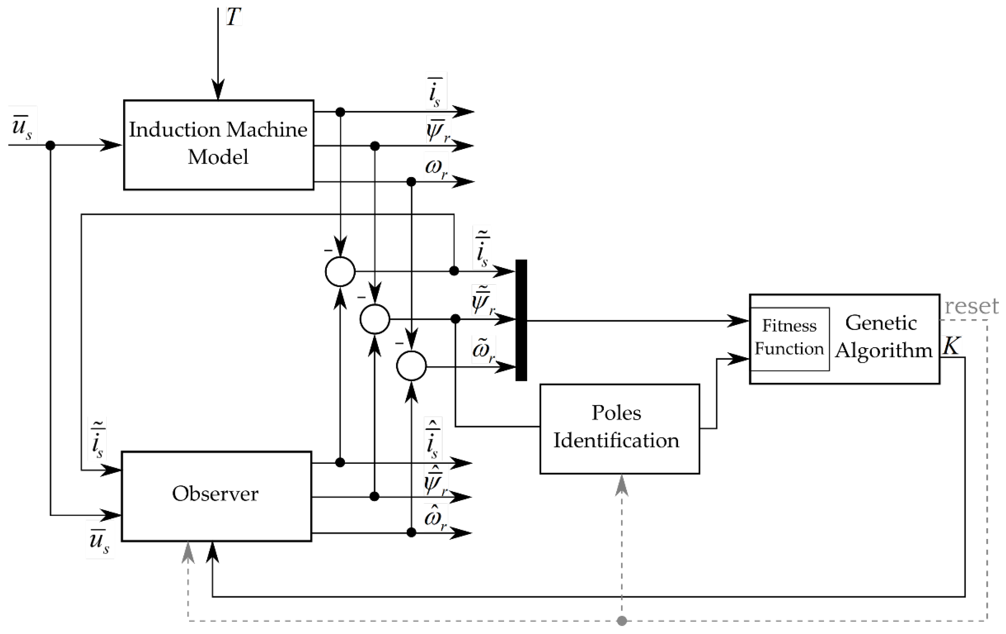
The main aim of this study is to propose a method of gains selection of the observer that does not require investigation of its mathematical implementation. The proposed solution is to determine dynamic properties based on the output signal, such as rotor flux estimation error. The block diagram of the proposed system is presented in Figure 2. During the evaluation step of the genetic algorithm each individual (gains set) is tested by performing a simulation. First, the observer is updated with an analyzed gains set and then the simulation is reset. The dynamic properties cannot be determined by measuring the steady state of the system. In order to attain the transient state an estimation error of the rotor flux is enforced by multiplying both compounds of this vector by 0.8. The signal, in this case module of the rotor flux error vector, is registered during the transient state. Based on this signal a system identification is performed and poles of the observer are estimated. The poles identification step is described in detail in Section 4. The final score is returned by a fitness function, defined in Section 5, based on estimation errors, and attained placement of the poles. After the evaluation is completed, the procedure is repeated for a new gains set.

Performing a whole simulation after reset, including transient states of induction machine during the start-up, may significantly increase the time needed to complete the gains selection. To speed up the gains evaluation, state variables of the machine and the observer are saved after steady state is reached. Afterwards, this state is restored every time a new gains set is loaded instead of performing an actual simulation reset.

4. Dynamic Properties Identification

The dynamic properties of the system can be determined by analyzing its response to a known input signal. It is possible to solve the problem by estimating the parameters of a linear discrete dynamic system. Such a system is described by the following equation:

$$y\left(k\right)+a_{1}y\left(k-1\right)+a_{2}y\left(k-2\right)+\dots +a_{n}y\left(k-n\right)=b_{1}u\left(k-1\right)+b_{2}u\left(k-2\right)+\dots +b_{n}u\left(k-n\right),$$

(11)

where k is discrete time, y(k) is the output signal, u(k) is the input signal, n is the order of the system, a₁, a₂, …, a_n, b₁, b₂, …, and b_n are system parameters.

Equation (11) can be rewritten as:

$$y\left(k\right)=\frac{B\left(q^{-1}\right)}{A\left(q^{-1}\right)}u\left(k\right),$$

(12)

where:

$$A\left(q^{-1}\right)=1+a_1{q}^{-1}+a_2{q}^{-2}+\dots +a_n{q}^{-n},$$

(13)

$$B\left(q^{-1}\right)=b_1{q}^{-1}+b_2{q}^{-2}+\dots +b_n{q}^{-n}.$$

(14)

The output of the system can be computed based on previous input and output samples using linear regression form:

$$\widehat{y}\left(k\right)=\varphi \left(k\right)\vartheta ,$$

(15)

where ϑ is a vector of parameters of the system:

$$\vartheta ={\left[\begin{array}{cccccccc}{a}_1& a_2& \dots & a_n& b_1& b_2& \dots & b_n\end{array}\right]}^T,$$

(16)

and ϕ holds previous values of the output and the input:

$$\varphi =\left[\begin{array}{cccccccc}-y\left(k-1\right)& -y\left(k-2\right)& \dots & -y\left(k-n\right)& u\left(k-1\right)& u\left(k-2\right)& \dots & u\left(k-n\right)\end{array}\right],$$

(17)

The system identification problem can be solved by finding a parameters vector ϑ that minimizes the distance between the vector of predictions $\widehat{y}$ and the vector of measured outputs y for a series of observations. A solution can be found using least-square estimation [26]:

$$\widehat{\vartheta }={\left({\Phi }^T\Phi \right)}^{-1}{\Phi }^{T}y,$$

(18)

where $\widehat{\vartheta }$ is the vector of estimated parameters, y is the output vector and Φ is the regressor matrix:

$$\Phi =\left[\begin{array}{cccccccc}-y\left(k-1\right)& -y\left(k-2\right)& \dots & -y\left(k-n\right)& u\left(k-1\right)& u\left(k-2\right)& \dots & u\left(k-n\right)\\ -y\left(k-2\right)& -y\left(k-3\right)& \dots & -y\left(k-n-1\right)& u\left(k-2\right)& u\left(k-3\right)& \dots & u\left(k-n-1\right)\\ \dots & \dots & \dots & \dots & \dots & \dots & \dots & \dots \\ -y\left(k-n_s\right)& -y\left(k-1-n_s\right)& \dots & -y\left(k-n-n_s\right)& u\left(k-n_s\right)& u\left(k-1-n_s\right)& \dots & u\left(k-n-n_s\right)\end{array}\right],$$

(19)

$$y={\left[\begin{array}{cccc}y\left(k\right)& y\left(k-1\right)& \dots & y\left(k-n_s+1\right)\end{array}\right]}^T,$$

(20)

where n_s is the number of observations.

The term ${\left({\Phi }^T\Phi \right)}^{-1}{\Phi }^T$ in Equation (16) is also known as pseudoinverse or Moore–Penrose inverse, hence the lest-square estimation can be written as:

$$\widehat{\vartheta }={\Phi }^{†}y,$$

(21)

where ${\Phi }^{†}$ is pseudoinverse of $\Phi$.

It is advised to compute the pseudoinverse directly instead of using Equation (18) due to a high impact of numerical errors. An accurate solution can be obtained by using a singular value decomposition [27]. The algorithms to compute pseudoinverse are implemented in most numeric computing environments such as MATLAB, GNU Octave or in the libraries for numerical linear algebra such as LAPACK.

After a successful system identification is performed, conclusions about dynamic properties of the system can be drawn by analyzing the poles of the system. The poles can be computed based on the coefficients of the denominator of the transfer function (12) by solving equation:

$$A\left(q^{-1}\right)=0.$$

(22)

The poles of the discrete transfer function λ_disc and are transformed from z-plane to s-plane:

$${\lambda }_{cont}=\frac{\ln \left({\lambda }_{disc}\right)}{T_s}.$$

(23)

where T_s is the sampling time used while collecting data for system identification and λ_cont are transformed poles. Such transformation allows placement of the poles analysis and estimation of dynamic properties, such as settling time or damping. Since poles are complex numbers, function ln(λ_disc) is a complex logarithm and can be computed as:

$$\ln \left({\lambda }_{disc}\right)=\ln \left(\left|{\lambda }_{disc}\right|\right)+i\arg \left({\lambda }_{disc}\right).$$

(24)

5. Fitness Function

The fitness function used in this study is similar to the one presented in [21] which is based on the placement of the poles of the observer. The minimized cost function has the following form:

$$f={\displaystyle \sum _{i=1}^n{w}_i}{f}_i(\lambda ),$$

(25)

where n is the number of objectives, λ is the vector of the poles of the observer, w is the vector of weights of the objectives and f is the vector of functions defining the objectives. The poles of the observer are complex numbers:

$$\lambda ={\sigma }_{\lambda }\pm i{\omega }_{\lambda },$$

(26)

where σ_λ is the rate of decay and ω_λ is the frequency of oscillation.

The first four objective functions are the same as in [21] and are described in detail there. Function f₁ is used to ensure stability of the observer:

$$f_1={\displaystyle \sum _{p=1}^6\left[f_{1r}({\lambda }_p)+f_{1i}({\lambda }_p)\right]},$$

(27)

where

$$f_{1r}=\left\{\begin{array}{ccc}-a_r({\sigma }_{\lambda }-{\sigma }_{max})& if& {\sigma }_{\lambda }\le {\sigma }_{max}\\ 0& if& {\sigma }_{max}<{\sigma }_{\lambda }<{\sigma }_{min}\\ a_{rs}({\sigma }_{\lambda }-{\sigma }_{min})& if& {\sigma }_{\lambda }\ge {\sigma }_{min}\end{array}\right.,$$

(28)

$$f_{1i}=\left\{\begin{array}{ccc}0& if& \left|{\omega }_{\lambda }\right|<{\omega }_{max}\\ a_i(|{\omega }_{\lambda }|-{\omega }_{max})& if& \left|{\omega }_{\lambda }\right|\ge {\omega }_{max}\end{array}\right.,$$

(29)

where coefficients σ_min, σ_max, and ω_max define allowable space on the s-plane and a_r, a_rs, and a_i define how fast the value of the cost function increases while poles move away from this area.

Function f₂ was defined to minimize the settling time of the observer by moving the dominant poles away to the left from the imaginary axis:

$$f_2=max\left({\sigma }_{\lambda 1},{\sigma }_{\lambda 2},\dots ,{\sigma }_{\lambda 6}\right).$$

(30)

The objective related to the function f₃ is to ensure proper damping of the observer to eliminate oscillations in the transient state:

$$f_3={\displaystyle \sum _{p=1}^6\left\{\begin{array}{ccc}{f}_{3a}({\lambda }_p)f_{3b}({\lambda }_p)& if& -\Re [{\lambda }_p]<|\Im [{\lambda }_p]|\\ 0& if& -\Re [{\lambda }_p]\ge |\Im [{\lambda }_p]|\end{array}\right.},$$

(31)

where

$$f_{3a}(\lambda )=\frac{\sqrt{2}\Re [\lambda ]}{\sqrt{{\Re }^2[\lambda ]+{\Im }^2[\lambda ]}}+1,$$

(32)

$$f_{3b}(\lambda )=e^{-a\left(\frac{\Re [\lambda ]}{r}-1\right)},$$

(33)

where r is the real part of the dominant pole.

Function f₄ minimizes gains values in order to decrease the influence of the stator current measurement errors:

$$f_4=\left|k_{13}\right|+\left|k_{14}\right|+\left|k_{23}\right|+\left|k_{24}\right|+\left|k_{33}\right|+\left|k_{34}\right|.$$

(34)

Functions f₁–f₃ are based on the placement of the poles of the observer and function f₄ depends directly on the values of the gains. In [21] values of those functions were evaluated using the placement of the poles acquired by computing the eigenvalues of matrix (6). In the proposed method, it is assumed that the matrix describing the dynamics of the observer is unknown. The placement of the poles is found using system identification by analyzing the response of the observer what requires performing a simulation. As a result, the signal of the real estimation error is known and can be directly used to define the objective function. Therefore, the fitness function was updated with a new objective f₅. Its goal is to minimize steady state error of the estimation:

$$f_5=\left|{\tilde{\psi }}_r\left(t_{end}\right)\right|,$$

(35)

where t_end is the end time of the simulation.

6. Results

The proposed gains selection method was verified for a speed observer presented in Section 2 and the machine with parameters is described in Appendix A. The simulations were carried out with a fixed sampling time of 10 μs. All variables, except of the time, are expressed in per unit values.

This section covers an analysis of the system identification method including the influence of the number of samples used during identification, the sampling time of the signal, and the order of the identified system. After those parameters are determined, the possibility of implementation of fitness function based on this method is verified using the genetic algorithm to find observer gains.

6.1. Influence of the Order of the Identified System

Prior to system identification, the order of the system n must be determined, which defines the number of the poles. The analyzed observer is described by three vector differential equations. Each vector is defined by two compounds; therefore, each vector represents two state variables. As a result, the order of the system is 6. It may be possible to approximate the system with a lower order system, therefore models of the lower order system were considered as well.

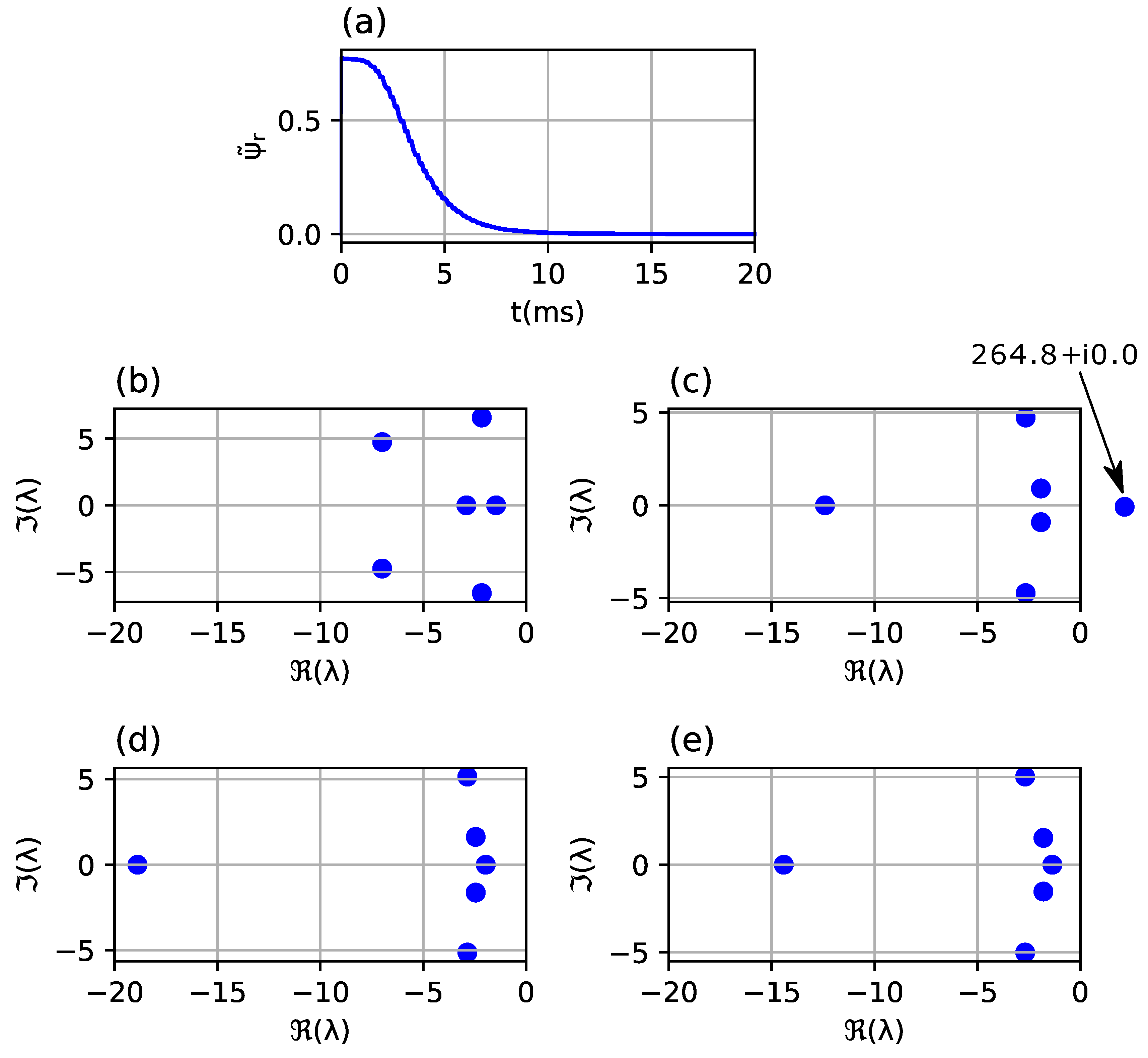
The system identification results are shown in Figure 3. The impulse response of the observer, caused by enforcing an 80% rotor flux estimation error, is shown in Figure 3a. Figure 3b presents poles acquired from computing eigenvalues of the matrix describing dynamics of the linearized observer (6). Identified poles for order of the system n equal to 6, 4 and 2 are presented in Figure 3c–e. The dynamics of the system are determined mainly by dominant poles (poles with the highest real part) and the poles on the left side on the complex plane have significantly less impact on the response of the system. For n = 6 (Figure 3c) the distance of the dominant pole of the identified system from the imaginary axis is close to the distance of the dominant pole of the linearized system. It is therefore possible to estimate a settling time of the observer based on identified poles. The rest of the poles, further from the imaginary axis, were not approximated as accurately due to their low impact on the output response. Such misplacement does not affect a gains selection algorithm as the fitness function is determined mainly through the placement of the dominant poles. In the case of n = 4 (Figure 3d) dominant poles remained at a similar distance from the imaginary axis as for n = 6, but for n = 2 (Figure 3e) the poles moved noticeably to the right. The settling times read from the transient response and estimated from placements of the poles using formula (36) are shown in

Table 1. Comparison of settling times for observer gains ensuring damped transient response read from the output signal and placement of the poles.

Transient Response	Linearized System	Identified System n = 6	Identified System n = 4	Identified System n = 2
7.2 ms	6.5 ms	7.0 ms	5.6 ms	14.5 ms

.

$$t_{settling}\approx 3T=3\frac{1}{\sigma },$$

(36)

where σ is a real part of the dominant pole.

It can be concluded from the flux error signal that observer gains ensure damped response. In case of poles calculated from linearized equations and poles of identified systems for n = 6, dominant poles are real poles that confirm the expected lack of oscillations in transient response. In the case of n = 4, dominant poles have a nonzero imaginary part but the ratio of the real to imaginary part is big enough to expect a damped system. The conclusions about system dynamics drawn from placement of the poles of identified systems for n = 6 and n = 4 are close to the real properties of the system read from the transient response.

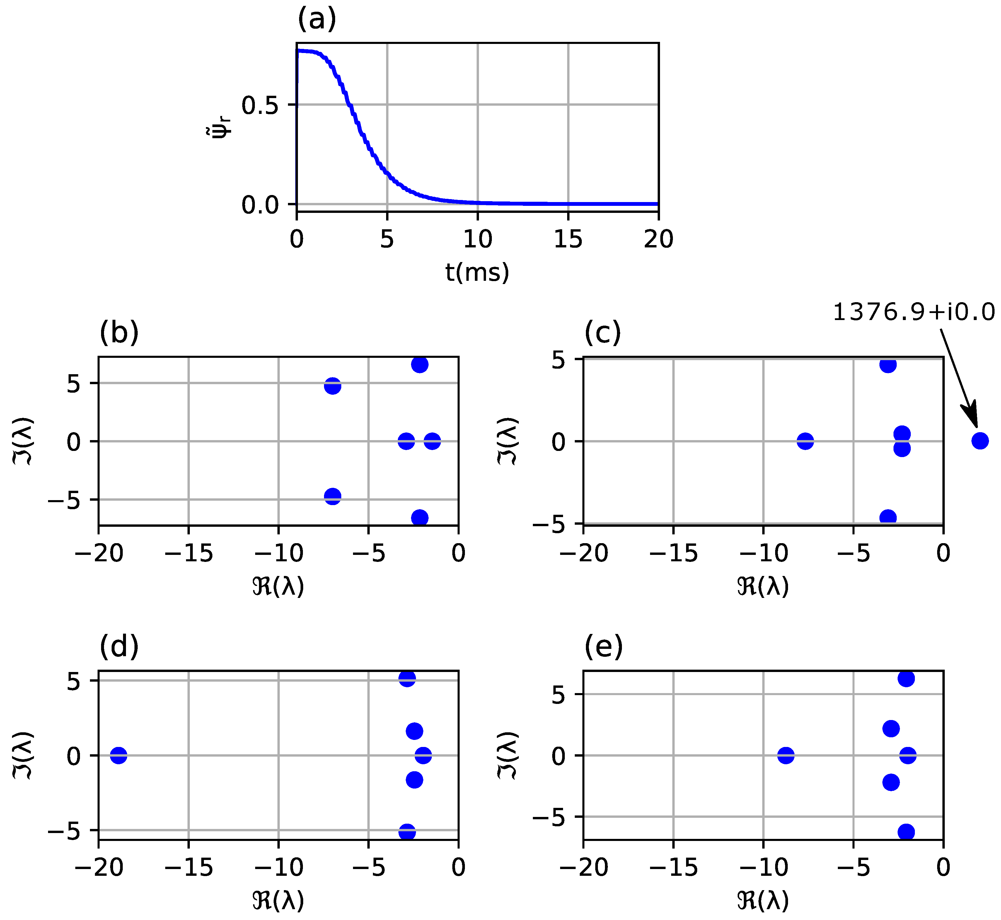
Similar studies have been performed for an underdamped system (observer with gains K_osc presented in Appendix B) with a longer settling time as shown in Figure 4 and

Table 2. Comparison of settling times for observer gains providing underdamped transient response read from the output signal and placement of the poles.

Transient Response	Linearized System	Identified System n = 6	Identified System n = 4	Identified System n = 2
19.9 ms	17.4 ms	17.6 ms	18.3 ms	21.5 ms

. In this case, the conclusions drawn from the placement of the dominant poles of identified systems for n = 6 and n = 4 describe the dynamics of the transient response properly, as previously, while for n = 2 the settling time is significantly longer. For that reason, it is advised to avoid using a low order system for identification in this application. The system of order equal to the order of the system of equations of the observer, in this case n = 6, as well as the reduced order of n = 4 yield sufficient results.

6.2. Influence of the Number of Samples on System Identification

The influence of the length of the signal used for system identification is presented in Figure 5. The study was performed for order of the system n = 6 and constant sampling time T_s = 150 μs. Results for three signal lengths are discussed:

• A total of 3.75 ms (25 samples): period shorter than settling time not covering steady state;
• A total of 15 ms (100 samples): period longer than settling time that covers transient and steady state;
• A total of 75 ms (500 samples): period significantly longer than settling time.

The signal covering the incomplete system response results in the poles of the identified system on the right side of the complex plane (Figure 5c) falsely suggesting its instability. In case of sample numbers high enough to cover both the transient and steady state, the system dynamics are properly identified, and results are reasonable even for very long signals where over 85% of the signal covers the steady state (Figure 5e).

For the purpose of gains selection using the proposed fitness function, it is safe to assume a high number of samples for system identification as a high share of steady state in the signal does not have a high impact on the results while the signal containing an incomplete transient state leads to wrong conclusions. On the other hand, gathering too many samples increases the time needed to complete gains selection. The genetic algorithm may evaluate fitness function thousands of times before the final gains set is found. Each fitness function call requires performing a simulation of the whole system in order to obtain the response signal used by the identification algorithm. Since the time needed to perform the simulation dominates the time of the fitness function evaluation, the gains selection algorithm is approximately proportional to the number of samples used for identification.

6.3. Influence of Sampling Period on System Identification

The results of the identification algorithm may be affected by the sampling period of the input signal. The influence of the sampling period is shown in Figure 6. The study was performed with a constant signal length of 15 ms and the order of identified system n = 6. The analyzed cases are T_s = 20 μs (750 samples), T_s = 150 μs (100 samples) and T_s = 500 μs (30 samples). For the sampling periods 150 μs (Figure 6d) and 500 μs (Figure 6e), it is possible to estimate the dynamics of the system based on the identified dominant poles. In case of short a sampling time (Figure 6c) one of the poles is on the right side of the complex plane that wrongly indicates instability. Reducing the sampling period too much may therefore make the identification algorithm to fail. Using the least-squares estimation to identify the system, it is required to gather the number of samples covering the transient state higher than the multiplicity of the order of the system [26]; therefore, the maximum sampling period is constrained by the shortest expected settling time of the observer.

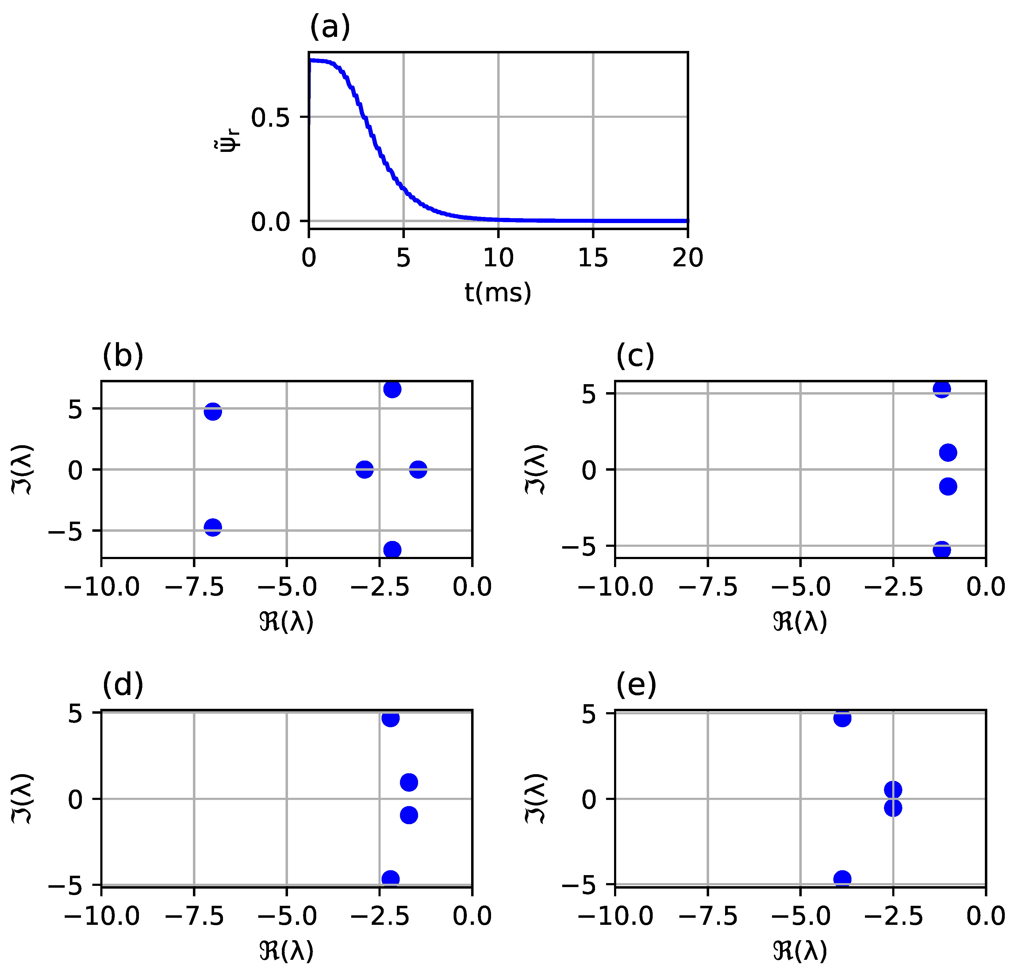
This study was repeated for the reduced order of the system n = 4. The results are shown in Figure 7. In this case there is no falsely unstable identification, even for the low sampling period. Since conclusions concerning the dynamic properties of the system based on the placement of the dominant poles are valid, it may be advised to use a reduced order of the identified system.

6.4. Gains Selection

During the gains selection the order n = 4 of the system used for identification of the dynamics of the observer was assumed as this is the lowest value that yields adequate results. The expected settling time for an induction machine speed observer with properly tuned gains is in range of a few milliseconds. The length of the signal processed by the identification algorithm was therefore defined as 50 ms to fully cover the anticipated solutions but also to be short enough to complete the gains selection in a reasonable time. The sampling period of that signal is 500 μs; therefore, it consists of 100 samples. The remaining parameters of the genetic algorithm and fitness function are presented in Appendix C.

A part of simulation results during the 1st and 10th generation of gains selection is shown in Figure 8. The impulse responses can be clearly seen for every newly evaluated gains sets. Some of the solutions yield a damped response with the settling time of few milliseconds while others deliver oscillations in an estimation error signal or even indicate instability. With higher generations the number of stable solutions increases. As it can be seen, in the 1st generation none of the gains sets yield stable observers while in the 10th generation unstable results do not appear that often.

As proposed in this study, the method was compared with the results acquired using the fitness function based only on the placement of the poles computed from linearized equations of the observer (6) which was described in detail in [21]. The convergence of the genetic algorithm for the two methods is presented in Figure 9.

The final gains sets found in one of the gains selection attempts for both methods are presented in Appendix D. The comparison of the dynamics of the solutions is shown in Figure 10. Both methods yield similar results with a damped response and settling time of 8 ms for fitness function based on linearized equations and 5 ms for the universal method proposed in this study.

The results presenting the performance of the observer in a wide speed range (up to double the nominal speed) are shown in Figure 11. The square wave load torque signal was applied as a disturbance in order to enforce transient states of the observer in the whole speed range. In case of gains set found using fitness function presented in [21] the impact of the load torque change is higher and results in higher estimation errors than in case of the gains set acquired using method proposed in the current study. It may be caused by a faster response of the observer using the second gains set (as seen in Figure 10). In the case of the gains acquired using the new method, the rotor speed estimation error does not exceed 0.5% of the nominal speed, even in a field weaking region.

The time needed to find observer gains using the proposed method is 13 min, compared with 10 s using method described in [21] where the placement of the poles is calculated from the matrix (6). In both cases the same number of generations and the same population size were applied. The significantly longer time needed for completing the gains selection in the case of the first method is caused by the necessity of performing a simulation for every individual while performing a genetic algorithm.

7. Discussion

The studies presented in this study confirm that the proposed method can be successfully applied to find gains of the speed observer. The presented fitness function evaluated by genetic algorithm is based only on the simulated output signal of the observer that ensures the versatility of the method as no knowledge of observer implementation nor prior preparation (such as linearization) is required. The system identification algorithm is used in order to estimate dynamic properties of the observer.

Least-squares estimation was used as an identification algorithm. In order to perform this algorithm three parameters must be defined: order of the system, sampling period, and length of the signal used for the identification. As presented in the study, the studies show that proper conclusions regarding the dynamics of the system can be drawn with a minimum system order of n = 4. Higher order systems increase the time needed for computation and tend to fail in the case of a low sampling period (high number of samples). The length of the signal used for identification should be high enough to cover the full transient state of the response as well as a part of the steady state. It is safe to assume that longer signals as steady state signal do not affect the results much, but signals that cover only the beginning of the transient state may lead to the wrong conclusions, and even falsely suggest instability. The sampling time should be short enough to ensure that the transient state includes at least n (order of the system) samples, preferably few times the order of the system.

Results show that the proposed fitness function copes well with the gains selection problem and the final solution yields similar properties as the solution found using the fitness function based on the analytical approach using the linearization of the observer. The main advantage of the proposed method is the lack of the need of analytical preparation, e.g., linearization. For the analyzed observer to find the linearized state matrix required for computing 36 partial derivatives of relatively complex equations and latter verification is a time-consuming task. Another advantage of the proposed method is the possibility of implementing quality indices based on a real system response, such as steady state estimation error, or estimation error at the end of simulation in case the steady state was not reached, e.g., due to instability. The linearized system is only an approximation, and it is possible that the conclusions drawn from the placement of eigenvalues of the linearized state matrix may be far from reality or the system may be reaching an equilibrium point that does not provide zero estimation errors. The proposed fitness function is immune to such conditions.

The main disadvantage of the method introduced in this study is that the length of time needed to complete the gains selection is about 80 times longer than the method based on the linearized system. The extra time needed to find the solution is caused by performing multiple simulations of the system. The algorithm completes within 13 min (on current personal computers) which is a reasonable period and makes up for the time needed to linearize the equations and verify the results that can be hours of work for qualified staff.