Assessment of Human Exposure (Including Interference to Implantable Devices) to Low-Frequency Electromagnetic Field in Modern Microgrids, Power Systems and Electric Transports

Abstract

Electromagnetic field emissions of modern power systems have increased in complexity if the many power conversion forms by means of power electronics and static converters are considered. In addition, the installed electric power has grown in many everyday applications such as wireless charging of vehicles, home integrated photovoltaic systems, high-performance electrified transportation systems, and so on. Attention must then be shifted to include harmonics and commutation components on one side, as well as closer interaction with humans, that concretizes in impact on physiological functions and interference to implantable medical devices and hearing aids. The panorama is complex in that standards and regulations have also increased significantly or underwent extensive revisions in the last 10 years or so. For assessment, the straightforward application of the limits of exposure is hindered by measurement problems (time or frequency domain methods, positioning errors, impact of uncertainty) and complex scenarios of exposure (multiple sources, large field gradient, time-varying emissions). This work considers thus both the clarification of the principles of interaction for each affected system (including humans) and the discussion of the large set of related normative and technical documents, deriving a picture of requirements and constraints. The methods of assessment are discussed in a metrological perspective using a range of examples.

1. Introduction

People interact with electrical systems more and more extensively, as passengers of electric transportation systems (not only railway and metro trains but also electric vehicles, for which the interaction is extended to the recharging process) and as users of a wide range of electrical appliances (induction cookers, drills, welders, battery chargers, etc.) and distribution systems (such as for the integration of renewable energy sources at home and work, in particular, photovoltaic panels). The higher power concentration and better performance usually call for a larger number of electric conversion stages, more advanced static converters with more intense operating current, and higher switching frequencies. The smaller size and smart deployment onboard imply in general shorter distance from the source, which combined with the more intense and frequent use imply a higher level of exposure overall. Conversely, the proliferation of standards and regulations to limit emissions and human exposure for equipment and installations has raised manufacturers’ awareness and improved design and layout at the same time.

The interaction of the human body with the electromagnetic (e.m.) field limited to the low-frequency range (as it will be better defined later in this Introduction) has been studied and modeled focusing on a set of biological and physiological mechanisms:

• Body current flow possibly interfering with the nervous system and other endogenous systems (such as retina, heart, etc.);
• Heating at a higher frequency due to dielectric losses and molecule movement;
• Mechanical forces on metallic implants in case of large field intensities;
• In general interference to implanted devices.

A comprehensive synthesis of such work appeared in the well-known ICNIRP (International Commission on Non-Ionizing Radiation Protection) publications, published between 1998 and 2020 [1,2,3,4,5]: such publications contain an explanation of the most significant mechanisms of interaction, resulting in the identification of the most relevant quantities internal to the body (basic quantities) and external (measurable reference quantities).

Frequency ranges were defined where such interaction mechanisms exert their most relevant effect, rationalizing the definition of limits and assessment methods to substantiate two sets of phenomena: low frequency, with induced body current and internal electric field, and high frequency, with contact current and heating. These phenomena are the so-called “acute effects”, that are directly measurable and for which there is a general consensus on the interaction mechanisms with the living being. They do not exclude long-term effects that need, however, more complex cohort studies and are in general characterized by a larger uncertainty. On this point, the findings and viewpoints are different and there is some deal of disagreement in the scientific community: there is no strong evidence that at an intensity lower than the prescribed limits there are significant adverse long-term effects, although there are results for instance showing statistically significant contribution (contributory cause) for the magnetic field at supply-frequency [6]. The exposure of population (and in particular children) to the nearby overhead power lines (OHLs) is a long-debated problem [7], although OHLs are just the most evident element of a national transmission and distribution grid, they were also recently developing as buried cable lines, especially at Medium Voltage level amid cities and suburban areas.

High-voltage OHLs are a source of electric and magnetic fields mostly at power frequency (namely 50 and 60 Hz): phenomena are well known and accurate estimates of field intensity and distribution can be obtained by various types of numeric models, once the geometry and the electrical quantities are known [8,9]. The calculation is particularly useful for estimation purposes, such as the identification of hot spots, both nearby lines and at substations [10]. Practically speaking, the electric field with its large wave impedance is attenuated by any even weakly conductive parts (including vegetation and the operator’s body), so that measured values may be affected by significant errors and calculated values turn out to be a valid choice. The magnetic field is also easily modeled when the geometry of conductors is simple and the results are quite accurate. Modern AC and DC microgrids and smart grids contain a large number of distortion sources, for which modeling of emissions and estimate of exposure may be numerically more complicated than at low frequency only.

Situations with intense static magnetic field are more and more common, as for medical diagnostic machines (e.g., Magnetic Resonance) and in case of large DC current flow (such as galvanic industrial processes, welding, and electrical discharge machining, DC railways and metros, DC grids and electric vehicles). With intense static magnetic fields, induction can occur when switching on and off of the source (transient) and with the body moving within a high-intensity field so that human exposure is of less concern. However, for what regards the protection of people wearing pacemakers (PMs), Implantable Cardioverter Defibrillators (ICDs), Cardiac Resynchronization Therapy (CRTs), and various other types of Implantable Medical Devices (IMDs), the general orientation is towards a low limit level of 0.5 mT [11], that potentially calls in cause all the aforementioned applications as relevant. For the other scenarios of exposure, excluding large-field diagnostics, however, current distortion may be significant and must be duly considered.

Protection of people with IMDs, besides a general concern for the public, is also a relevant problem for accessibility and safety of the workplace, where the range of sources is wider, separation distance may be shorter, and duration of exposure depends on tasks and work shifts. In addition, there is also a precise duty and responsibility of the employer that has fostered the standardization activity of the last 10 years or so. The IMDs standards are issued by IEC/CENELEC and ISO and need a specific discussion with the aim of synthesizing a clear regulatory framework in terms of limits of environmental e.m. field derived from known immunity characteristics of the device (and integrated then with the requirements for human exposure).

As part of the medical devices that can be worn by the public and workers, hearing aids should be included, for which the assessment procedure must consider the applications (listening to music, normal conversation, hearing alarms, and escape instructions) and the related sound quality and intelligibility requirements. Performance and quality standards [12,13], in fact, may provide different signal-to-noise ratio requirements that should be critically discussed to appraise the exposure on a case-by-case basis.

Adequate and complete measurement procedures for quantitative assessment of exposure are particularly relevant in recent times with modern electric systems putting relevant sources in closer contact with the person and in particular with the general public.

Modern microgrids and power conversion systems are extensively used for domestic and industrial applications, featuring the integration of various sources (e.g., photovoltaic panels, fuel cells, and co-generation) with various types of static converters and with significant power concentration, especially relevant considering the large nominal current. As mentioned, commutation byproducts and harmonics fall well within the several kHz frequency intervals of minimum exposure limits.

Electric road vehicles and their wireless charging systems are another peculiar exposure scenario, characterized by proximity to the source of emissions (accompanied by a pronounced field gradient) and a significant amount of high-frequency components, including the wireless power-link resonant [14,15,16,17,18,19,20]. Link frequencies have been standardized [21] to the ranges described in

Table 1. Wireless Power Transfer for Electric Vehicles: standardized frequencies, power levels, and magnetic field emissions.

Freq. Range [kHz]	Power Level [kW]	Application
19–21	>20	S. Korea, UK, Germany
59–61	>20	S. Korea, UK, Germany
79–90	3.7–20	Worldwide
100–119 119–135 135–140 140–148.5 148.5–300	<0.15	Worldwide
36–40	—	under disc. CISPR
55–65	—	under disc. CISPR

: the most common ranges are between 19 and 90 kHz, with one remaining range going up to 300 kHz. Higher ranges are used for wireless power transfer of applications other than electric vehicles and are characterized by a much lower power level (e.g., charging of tools and appliances).

Electrified transports (trolleybuses, trams, metros and railways) may cause relevant exposure on-board for workers and passengers [22,23,24,25], they can be possibly exposed also when standing at the platform, for which the EN 50500 [26] distinguishes suitable selections of measurement points. It has been observed that the frequency range limited to 20 kHz [25] does not capture the whole relevant set of emissions, in particular for new technologies and power drives [27]. In this sense, the IEC 62597 [28] (based on the EN 50500) was extended in 2011 to the frequency range of 100 kHz.

Lastly, Short-Range Devices (SRDs) are a wide class of wireless devices conceived for the exchange of information at a reduced distance, using inductive transmission and reception systems, such as coils and loops with an operating frequency range beginning at 9 kHz. A well-known example are Electronic Article Surveillance (EAS) systems that protect, for example, shop and supermarket products, but they are outside the scope of this review. Other forms of SRD communication are (or could be) used for tariff metering and toll collection, alarm systems, wireless voice links, access control, proximity sensors, signaling, and train-wayside communication, etc.

SRD emissions are subject to limits for a matter of EMC and interference with other equipment nearby [29], usable also to evaluate exposure and interference to IMDs at a short distance. The values in Table 2 of the EN 300 330 [29] have been recalculated for a 1 m distance, as shown in Figure 1, using the same approach of the EN 300 330, that applies a full third-order assumption (1/r³) with all emitters operating in the reactive field region up to 1 MHz. The correction factor in the Annex H of the EN 300 330 is in fact 31.47 dB passing from 10 m to 3 m; it may be extrapolated to 60 dB (three orders of magnitude) if the distance is reduced to 1 m. As seen, at 1 m the values below 150 kHz are very close to the ICNIRP 1998 reference levels for the general public (5 A/m), then relaxed in the 2010 version to 21 A/m.

At a shorter distance from the e.m. field source, not only is the expected intensity larger (implying a lower margin with respect to the limit as for measurement error and uncertainty) but also the whole body exposure features a field gradient, with the intensity varying significantly along the exposed volume. This has implications not only on the number of measurements to take and the accurate positioning of the probes but also on the consequences of the implicit approximations of commonly used procedures, such as spatial averaging over body volume.

The modern electric systems exemplified above are not only characterized by some amount of harmonic distortion but also make use of multiple switching converters and smart modulators so that exposure is commonly characterized by multiple spectral components (multi-frequency exposure) and impulsive signals, whose processing from a pure Fourier standpoint is troublesome [31,32] and would be better assessed using a time-domain approach, as exemplified in [25,33].

For such electric systems, the emissions reviewed so far are relevant in the lower part of the vast frequency range that characterizes human exposure and is stigmatized by the 300 GHz upper limit of ICNIRP guidelines [1,4]. For agreement with the usual subdivision, the upper-frequency limit for this review should be fixed to 100 kHz. The upper boundary of the relevant low-frequency range may be yet assumed conservatively loosely positioned somewhere in the hundreds kHz range, based on the following considerations: (i) such a 100 kHz boundary is purely conventional, (ii) spectral emissions from some conversion apparatus may be shifted with relevant intensity to the higher frequency, and (iii) there is no abrupt transition of the mechanisms of exposure across the said 100 kHz boundary. Conversely, all the reviewed apparatus and systems are not intentional emitters of radiofrequency e.m. field, as occurs for a wide range of radio and smart devices that are widely diffused and feature a rapid technological evolution, culminating in wearable smart devices and antennas deeply interacting with body electromagnetic characteristics [34] and in the wireless LAN, 4G and 5G systems [35,36]. In this case, the prevalent mechanism of exposure is thermal, but some parameters and tissue characteristics are common to the present low-frequency domain, although to quantify at a higher frequency.

ICNIRP publications have been endorsed and incorporated at various levels by EU Directives (besides IEC/CENELEC standards), warranting the cogency of a regulation. Another complete set of standards more or less in agreement with these limits and frequency ranges is the ANSI/IEEE C95 [37,38,39,40]. Differently, national regulations may decide a significant change with respect to levels established in standards and guidelines, often remaining as the underlying reference: it is the case of many European countries although overall EU Directives exist, distinguishing residential and occupational margins, or specific limitation of electric and magnetic field exposure [41]; in Russia, there is a strong dependency on duration (dose) also for low-frequency exposure [41]; Australian ARPANSA has aligned low-frequency limits to ICNIRP 2010, but has issued a standalone standard for high-frequency exposure above 100 kHz [42]; Canada has issued the “Safety Code 6” in 2015 moving away from the ANSI/IEEE limits and taking up the ICNIRP limits between 3 kHz and 10 MHz; Japan has for a long time promoted studies and regulations for limitation of exposure, participating consistently to ICNIRP studies [43].

The Introduction has discussed the subject offering an overview of the possible sources of emissions from the point of view of the application. Section 2 instead introduces the interaction of the e.m. field with the subject or device, identifying relevant elements of quantification of phenomena. Section 3 considers the applicable standards, providing limits and requirements for human exposure, interference to IMDs and to hearing aids. The objective is to synthesize a set of requirements that define the scope of the measurement and assessment procedures. Section 4 then discusses such scope, having focused on low and medium frequency, representative of the sources and emission mechanisms reviewed so far. The characteristics of suitable instrumentation are reported, with emphasis on uncertainty and its impact on the assessment of compliance. Case studies and examples are referenced for clarification and demonstration purposes throughout this work.

There have been reviews of human exposure to e.m. field [7,41,44], but the present work stands out for the coverage of interference to IMDs and hearing aids (addressing overall the impact on humans), for the more complete normative panorama and for focusing on measurement methods and example cases.

2. Principles of Interaction and Interference Coupling

This section focuses on the physical principles that have been identified in the literature and are the basis to establish e.m. field limits to prevent adverse effects to the body (for human exposure), the implantable device, or the hearing aid.

2.1. Interaction of Electromagnetic Field with Subject’s Body

The mechanisms of interaction have been discussed in authoritative references and in particular, the ICNIRP guidelines report a very good overview [1,2,3,4,5]. The overall frequency range that is in principle almost unbounded (up to 300 GHz) has been subdivided into convenient sub-intervals, within which the examined phenomena take a clear connotation and for which typical sources and exposure scenarios may be identified. The objective is understanding the interaction of external e.m. quantities (namely electric and magnetic field, limb current and contact current) with the internal quantities interacting with the body physiology: the internal quantity affecting electrically sensitive cells (such as the nervous system) is the internal electric field E_i. It is quite difficult (or impossible) to measure so that the relationship between the external and internal electrical quantities is established by means of validated models. The internal quantity E_i is subject to limits named by ICNIRP Basic Restrictions (BR), assigned to different types of tissues, as shown in Table 2 (the IEEE refers to them as Dosimetric Reference Levels). Limits for external quantities, named Reference Levels (RL) by ICNIRP and Exposure Reference Levels (ERL) by IEEE, are then extrapolated using models with a cautious approach (discussed later in this section). Similarly, and related to E_i, is the internal current density J_i, flowing in specific body local areas or through the entire body or limbs.

In the determination of the basic restrictions, the most relevant tissues and organs are the Peripheral Nervous System (PNS), the Central Nervous System (CNS), the retina (for the induction of phosphenes), and in general the brain and the heart. In some cases, basic restrictions are derived overlapping ascertained adverse health effects with unpleasant or nasty reactions, which may also be disturbing or troublesome in some occupational scenarios. An external electric field in the order of 5 kV/m is perceivable and 5% of volunteers found intensities of 15–20 kV/m annoying [3]. Nerve stimulation was analyzed in some studies and findings of threshold E_i values ranged between 2 V/m [45] to 4–6 V/m [46] for power frequency stimulation. A 6.15 V/m peak excitation threshold is similarly assigned to 20 μm nerve fiber by the sec. B.2.1.9 of the IEEE C95.1. The response of CNS and PNS is different for which BRs (or DRLs) are set up to about 300–400 Hz for ICNIRP and 750 Hz for IEEE with attention to protecting the former and focusing on PNS above it [47].

Departing from the power frequency interval, organs and biological systems all show a reduction of sensitivity, so that stimulation thresholds increase above about 1 kHz (due to shorter time available for the accumulation of electric charge on the nerve membrane) and below about 10 Hz (due to the adaptation of a nerve to a slowly depolarizing stimulus) [3]. Cardiac stimulation and fibrillation occur at a larger intensity and have not received specific limits by ICNIRP.

A complementary effect is the formation of retinal phosphenes with maximum sensitivity around 20 Hz: the E_i threshold value was found between 50 and 100 mV/m, corresponding to an external magnetic flux of 5 mT. The lower sensitivity, but the higher induction effect for increasing frequency, have been weighted and combined to derive the reference levels for this particular phenomenon. At the same frequency, other studies [48,49,50] carried out at larger E_i values have reported evidence of influence to the visual and motor cortices, slightly affecting visual processing and motor coordination.

These effects are well-established acute effects verifiable in the short term. From a different long-term standpoint, moving away from the details of the physiological interaction and carrying out volunteer studies or residential/occupational epidemiological studies, results for impact on the endocrine and cardiovascular system, for neuro-degenerative disorders, and for adverse reproductive outcomes are negative or inconsistent. Similarly, for cancer, the general result is negative, also for those studies devised to replicate and verify older research in the 1980s and 1990s claiming association with long-term exposure to the power-frequency magnetic field. For childhood leukemia, the situation is slightly different in that there are some studies showing a weak association in terms of increased risk [3,6], although a causal link has not been identified yet and selection bias, as well as some confounding, might explain the results, according to WHO [51].

For these reasons, the ICNIRP chose not to include any reference levels nor guidelines to limit the exposure to prolonged exposure effects. A cautious approach was nonetheless followed when determining the reference levels for the identified acute effects: for nervous system stimulation, the average 4 V/m from scientific studies has been reduced by a safety factor of 5 already for occupational exposure (general public levels are even lower, also by about a factor of 5). The threshold for phosphene generation is considered a warning phenomenon for other more serious impacts on brain functions and is applied to occupational exposure (where such transient phenomena might be tolerated with suitable training and awareness), and to the general public (reduced by a factor of 5). A factor of 5 assuming median levels from the considered studies is more conservative than the multiplying factor of 2.1 and 3.1 for ventricular fibrillation and perception/pain, respectively, adopted by Table B.6 of the IEEE C95.1 [39], for the 99th percentile. Similarly, the derivation of DRL at low frequency for continuous-wave excitation is based on a safety factor of 3 with respect to the excitation/reaction thresholds (Table B.7 of the IEEE C95.1 [39]). To cover extremely sensible persons the IEEE C95.1 indicates also a lower-tier safety factor of 9. The ICNIRP factor of 5 corresponds thus approximately to the geometric mean of the two IEEE safety factors.

Regarding the derivation of reference levels, the adopted conversion factors with the basic restriction for E_i and J_i show an additional, but reasonable margin. Assuming the worst-case orientation of the body with respect to the external field (parallel and perpendicular to body axis for the electric and magnetic field, respectively), results reported in [52] show a significant variability for the magnetic field orientation front-to-back, top-to-bottom, and side-to-side (yet always keeping the direction of field straight): top-to-bottom leads always to lower values by about 10% to 35% with respect to the average of the other two.

For the use of body models and the collection of resulting values, it is important to observe two other sources of variability:

• The physical characteristics of the body models representing persons with different circumference and males/females (male results on average with 25% larger current density results); considering the specific publications and the reported results, also the use of, for example, European (Norman and Naomi) and Japanese (Taro and Hanako) body models has an influence, with 52 different tissues for the latter compared to about 38–41 for the former, and with the classification of white and grey matter only in the Japanese models [52].
• The methods to process the model voxels values, depending on the reference guideline/standard: ICNIRP requires calculations on 2 × 2 × 2 mm³ elements taking the 99th percentile value and IEEE the maximum of 5-mm long filaments to compare to the BR or DRL, respectively [47]. When operating spatial averaging over larger volumes and surfaces, such as with 1 cm² for the calculation of the current density J_i, the collection of adjacent mesh cells for an equivalent 1-cm² area may include or not non-nerve tissues and this causes a large variation in the order of 5 to 12, leading to larger, but more stable, values when non-nerve tissues are excluded [52].

A very good review of human body models and calculation methods can be found in [53], where a thorough comparison of E_i calculated values shows a maximum variability of 10% to 30% depending on tissues and organs. Table 2 reports a set of conversion factors between external quantities (E- and B-field) and internal quantities (E_i and J_i).

By observing the values in Table 2, it is possible to conclude that the variability of the conversion factors is large, also for the same body model and same study, only considering the resulting values for different portions of the same type of tissue. In a conservative perspective, when establishing RLs or ERLs reasonable worst-case values are considered, which will bring to set unique limits for the external quantities bringing the parts with the largest conversion factors to compliance, but applying a significant margin for the remaining part of the body. In other words, the specific case of exposure may be non-compliant if the reference levels for the external field quantities are considered, but compliant with the margin if the internal quantities (dosimetric) are considered.

Table 2. Conversion factors between external field at 50 Hz and internal quantities (E_i and J_i) as resulting from various types of models [3,52,53,54,55,56,57].

Reference	Body Areas and Conditions	Internal E-Field Ei		Internal Current Density Ji
		B-Field [mV/m/mT]	E-Field [mV/m/(kV/m)]	B-Field [(mA/m2)/mT]	E-Field [(mA/m2)/(kV/m)]
ICNIRP 2010 [3]	Brain	23–33	1.7–2.6	—	—
ICNIRP 2010 [3]	Skin	20–60	12–33	—	—
Hirata 2009 [52]	Taro, Cerebro- Spinal Fluid	—	—	74.8–81.5	—
Hirata 2009 [52]	Taro, Skin	312	—	—	—
Hirata 2009 [52]	Taro, spinal cord /grey matter	27.7–89.1	—	2.26–22.4	—
Hirata 2009 [52]	Hanako, Cerebro- Spinal Fluid	—	—	50.3–57.4	—
Hirata 2009 [52]	Hanako, Skin	97.7	—	—	—
Hirata 2009 [52]	Hanako, spinal cord/grey matter	25.9–65.1	—	2.25–16.7	—
Hirata 2009 [52]	Norman, grey matter	30.7–48.6	—	3.32–3.56	—
Hirata 2009 [52]	Naomi, grey matter	25.7–31.4	—	2.81–2.98	—
Dimbylow 2000 [56]	Brain	—	—	—	0.176
Dimbylow 2000 [56]	Muscle	—	—	—	0.832
Dimbylow 2007 [57]	Naomi, pregnant foetal body (13–38 w)	9.11–21.4	1.12–1.56	3.78–7.34	0.29–0.47
Dimbylow 2007 [57]	Naomi, pregnant foetal brain (13–38 w)	5.52–24.7	0.67–1.62	0.77–3.37	0.11–0.19

Table 2. Conversion factors between external field at 50 Hz and internal quantities (E_i and J_i) as resulting from various types of models [3,52,53,54,55,56,57].

Reference	Body Areas and Conditions	Internal E-Field Ei		Internal Current Density Ji
		B-Field [mV/m/mT]	E-Field [mV/m/(kV/m)]	B-Field [(mA/m2)/mT]	E-Field [(mA/m2)/(kV/m)]
ICNIRP 2010 [3]	Brain	23–33	1.7–2.6	—	—
ICNIRP 2010 [3]	Skin	20–60	12–33	—	—
Hirata 2009 [52]	Taro, Cerebro- Spinal Fluid	—	—	74.8–81.5	—
Hirata 2009 [52]	Taro, Skin	312	—	—	—
Hirata 2009 [52]	Taro, spinal cord /grey matter	27.7–89.1	—	2.26–22.4	—
Hirata 2009 [52]	Hanako, Cerebro- Spinal Fluid	—	—	50.3–57.4	—
Hirata 2009 [52]	Hanako, Skin	97.7	—	—	—
Hirata 2009 [52]	Hanako, spinal cord/grey matter	25.9–65.1	—	2.25–16.7	—
Hirata 2009 [52]	Norman, grey matter	30.7–48.6	—	3.32–3.56	—
Hirata 2009 [52]	Naomi, grey matter	25.7–31.4	—	2.81–2.98	—
Dimbylow 2000 [56]	Brain	—	—	—	0.176
Dimbylow 2000 [56]	Muscle	—	—	—	0.832
Dimbylow 2007 [57]	Naomi, pregnant foetal body (13–38 w)	9.11–21.4	1.12–1.56	3.78–7.34	0.29–0.47
Dimbylow 2007 [57]	Naomi, pregnant foetal brain (13–38 w)	5.52–24.7	0.67–1.62	0.77–3.37	0.11–0.19

Although an easy concept, the direct measurement of the internal quantities on a living subject is possible only for the current density J_i, and in this case, the measurement can only be applied to the whole body (e.g., current through the feet on a conductive platform) or to the limbs (as in the case of contact current exposure measured using clamping probes or shunt within the circuit establishing the electric contact). Contact current is a measurable quantity, extensively used together with touch voltage for electrical safety assessment, both at DC and AC [54,55]. The electric field E_i, however, cannot be measured directly on humans and can be more accurately determined only by refining and tuning to the present situation a verified numeric model. For this reason, to follow an experimental approach, phantoms are extensively used that represent the composition in terms of density and electric properties of the typical tissues of the human body: they can be instrumented with probes for both E_i and J_i.

2.1.1. Static Fields

Static field exposure is peculiar and is covered by a specific ICNIRP guideline [5], whereas IEEE C95.1 [39] incorporates limits for DC or extremely low frequency. Typical cases are those of Nuclear Magnetic Resonance diagnostics and to a lesser extent, inductive circuits with large DC current flow, such as onboard trains, at photovoltaic (PV) parks, large power DC grids, including large battery systems, and in relation to galvanic plating and other electrochemical processes. The tolerated values are quite large to have static field “forgotten” most of the time, although a lower limit value must be considered aiming at the protection of pacemakers (see sec. 2.2), and this is usually a critical point. Despite the absence of induction per se, the considered large intensity is able anyway to cause induction with a moving body or at application/removal of the field. The impact on human physiology can be synthesized as follows.

• Magnetic induction:
  • Lorentz forces on mobile ionic charges, as for flowing blood, thus causing current flow and internal electric field build-up; in [5] for an external magnetic induction field of 5 T an induced current density of 100 mA/m² is estimated, that corresponds to the 10% of the maximum endogenous current from cardiac electrical activity;
  • By virtue of Faraday’s law an external time-varying field, as well as movement within a static magnetic field, can both induce an electromotive force; the magnitude of induction is proportional to the velocity of the movement and amplitude of the gradient. At a 3 T intensity, there are several reported episodes of nausea and phosphenes for patients and workers around magnetic resonance machines. A calculation for a 0.5 m/s speed of movement and a field intensity of 4 T gives the E_i lower bound of 2 V/m for peripheral nerve stimulation, which we saw is at the threshold for phosphenes generation.
• Magneto-mechanical effects:
  • Besides the orientation of paramagnetic molecules (that is not considered to affect biological material remarkably), magnetic field gradient can exert a translational force on paramagnetic and diamagnetic materials, the difference being in the force sign. What matters is the product of the field intensity B and its gradient dB/dx, for which a reduction of blood flow in rats was observed for a combination of B = 8 T and product B × dB/dx = 200–400 T²/m (i.e., a gradient of 0.25–0.5 T/cm).

2.1.2. Field at Power Frequency, Harmonics and Supraharmonics

Power frequency electric and magnetic fields may affect workers and the public, including situations with long exposure, such as home exposure caused by overhead power lines, but also locally deployed power transformers and modern systems of domestic generation. The attention is, in general, focused on 50/60 Hz values for the much higher chance of reaching large intensity, compared to other frequencies nearby, although physiological response extends below and above mains frequency. For power frequency and harmonics the main mechanism of interaction is induction, and for this reason, limit values progressively reduce with increasing frequency to keep induced current density J_i and resulting E_i at a constant safe level.

A linear dependency on frequency may be reasonably assumed over the extended frequency range up to 10 MHz, as shown by Dimbylow [56], for J_i as induced by the external E-field on a grounded or isolated body.

As a brief note, not all tissues and organs react in the same way, for which the cardiac muscle has a maximum sensitivity around mains frequency that drops significantly above the second harmonic, as in general muscles are less receptive than nerves at a higher frequency. The mentioned phosphenes that represent the lowest threshold of excitation and their protection is thus the most restrictive have a peak response around 20 Hz, that then reduces progressively with frequency, so that at about 400 Hz it is peripheral nerve stimulation that sets the tolerability thresholds.

The induction mechanism, formerly covered up to 100 kHz [1], has been fully extended up to 10 MHz in the ICNIRP 2010, in agreement with the extension of the new IEEE C95.1 [39] up to 5 MHz (the boundary of 100 kHz remaining for the electric field ERLs). It resulted that for the entire range a quasi-static Maxwell modeling may be used, neglecting propagation and reactive effects [47,58,59]. It is observed that for the other interaction mechanism, limits for heating of tissues (usually ascribed to high-frequency and radiofrequency) begin at 100 kHz in [4,39], showing a significant overlap of restrictions for the two mechanisms for two decades of frequency.

For the complete characterization of the electrical systems considered in this review, an extension beyond the older conventional boundary of 100 kHz is indeed advisable based on some considerations:

• The former decision of dividing low- and high-frequency intervals at 100 kHz was a matter of convenience.
• The relevant emissions characterizing modern power systems and connected equipment are spread over a significant frequency interval. As an example, the emissions of large power converters on-board a DC electro-train of 25 years ago in [25] were observed up to about 100 kHz, and high-frequency spectrum pollution is expected to increase with faster technology; for electric vehicles emissions E- and H-field levels extend at the largest values up to the main resonance frequency in the order of 1 MHz [60]. It was similar for large power drives [61].
• Conducted emissions are regulated by EMC standards using the 150 kHz boundary, that separates the so-called supraharmonics from the radiofrequency conducted emissions; by experience, conducted emissions of large power converters are significant up to some MHz at most, also as a consequence of internal cabling resonance [60], that turns out to be a significant element that affects the intensity of emissions in the medium frequency range.

2.2. Interference to Pacemakers and Other Implantable Devices

PMs and ICDs in particular have been long studied for various types of EMI, connected to both the common use at home and at the workplace, but also at hospitals and during medical practice. Studies cover about 40 years since the early 1980s. IMDs models have changed through the years, improving performance and durability, reducing size, and optimizing wiring and deployment, so that a general improvement of the immunity can be stated, with the older experimental results pointing at more critical situations.

At present, these devices have an EMC qualification carried out by the manufacturer for the purpose of certification, including tests with levels and parameters that characterize the device immunity. In general, they are more susceptible to a low-frequency magnetic field, rather than RF e.m. field for which they are effectively shielded, although some issues due to near-field radio transmission by RFID readers and telemetry for hospitalized patients have been reported [62].

EAS systems emissions occur in the upper part of the low-frequency range and are impulsive: episodes of interference were reported back in the 1990s [63,64,65] raising the concern also for such type of interference, and fostering technological development (such as the use of hardware and software filters) in modern IMDs, besides a revision of suitable limits and exposure verification procedures [66].

Immunity test levels and methods, as per applicable EMC standards, are discussed later in Section 3.2. The situation with respect to human exposure limits has evolved, in that with older lower reference levels, it could be stated that compliance to the latter was a sufficient condition; newer reference levels are less restrictive and there is no absolute coverage for the entire frequency interval (besides the already commented static field), as it will be shown later in Figure 6.

The coupling of interference occurs with two mechanisms: direct illumination of the device body and induction on the connecting leads. The latter is the most relevant with a significant improvement achieved by miniaturization and optimization of wiring layout: passing from unipolar to bipolar wiring reduces the exposed area and the induced noise by an order of magnitude; the overall length of the circuit is optimized with implantation in the left pectoral.

The operation of a PM or ICD is complex, with several operating modes and criteria for enabling/disabling a certain kind of stimulus: this means that there are various levels of susceptibility and interference, and the device parameters can be optimized to reduce chances of disruption of its operation. Such parameters are in synthesis the sensitivity threshold and the frequency response for which fibrillation is detected. Such devices can also notch filter 50 or 60 Hz hum due to mains induction or, worse, contact current (e.g., residual current of a leaking electrical appliance). Circuit arrangement and exposure to an external low frequency e.m. field for a pacemaker are depicted in Figure 2.

The EN 50527 standards report two expressions for pacemaker disturbance in relation to the external field intensity (they are the counterpart of the conversion factors shown in Table 2 for human exposure) [67,68,69]. Some clarification is necessary, as the E-field formulas reported in Ref. [67] were those of the old version 2011 (EN 50527-1), now transferred to the EN 50527-2-1 and -2-2 [68,69] with some changes. It is noted that exemplified by this normative evolution (and other similar ones, such as the change of reference levels between the 1998 and 2010 ICNIRP publications), attention must be paid when collecting and comparing previous studies.

For the electric field induction at low frequency (nominally at 50 Hz, but anticipating a linear scaling factor for frequency, discussed below) the net induced voltage is due to the difference in length of the tip and the ring wires (the blue and red lines in Figure 2), picking up the potential gradient within the tissue, which happens to be characterized by a low electrical conductivity, giving rise to a non-negligible voltage gradient.

For magnetic field induction (again including a linear frequency scaling) the equivalent area for the bipolar configuration is found using an area with angular sector shape centered on the PM and with an angle of aperture given by the distance between the tip and the ring.

The formulas reported in the Annex E of the EN 50527-2-1 [68] are:

$$V_{ind,pp,unip}[\mathrm{nV}]=4.4f E_{ext,p}\hspace{1em}\hspace{1em}{V}_{ind,pp,bip}[\mathrm{nV}]=0.23f E_{ext,p}$$

(1)

$$V_{ind,pp,unip}[\mathrm{nV}]=360f H_{ext,p}\hspace{1em}\hspace{1em}{V}_{ind,pp,bip}[\mathrm{nV}]=18f H_{ext,p}$$

(2)

where E_ext,p and H_ext,p is the peak value of the external electric and magnetic field in V/m and A/m, respectively; f is the frequency in Hz; the range of validity is 16 Hz to 150 kHz for the E-field formula and 16 Hz to 5 MHz for the H-field formula. As a note, for the E-field formula, a barefoot grounded 2-m tall person has been assumed, but not with raised arms (equivalent to a person wearing shoes, but with raised arms).

Regarding simultaneous exposure to an E- and H-field, the EN 50527-2-1 indicates the addition of the absolute values of the two terms for unipolar (or for bipolar) wiring, using E_ext,p (t) and H_ext,p (t) as the time-varying values of the E- and H-field. This is valid only between 16 and 60 Hz. At higher frequency, there is no formula between 60 Hz and 150 kHz, and for the range 150 kHz to 5 MHz the addition of E- and H-field components is quadratic, as below.

$$V_{ind,pp,unip}[\mathrm{nV}]=36f \sqrt{{10}^6{H}_{ext,p}^2+E_{ext,p}^2}$$

(3)

One of the parameters of the above formulas is the exposed area, which must be assigned reliable and correct values. It is evident how they instead can vary between different implantations (left pectoral, right pectoral, abdominal, the latter not advisable and for clinical environment only) and geometry of tip and ring for bipolar leads. The EN 50527-2-1 and -2-2 fix the values of the parameters as:

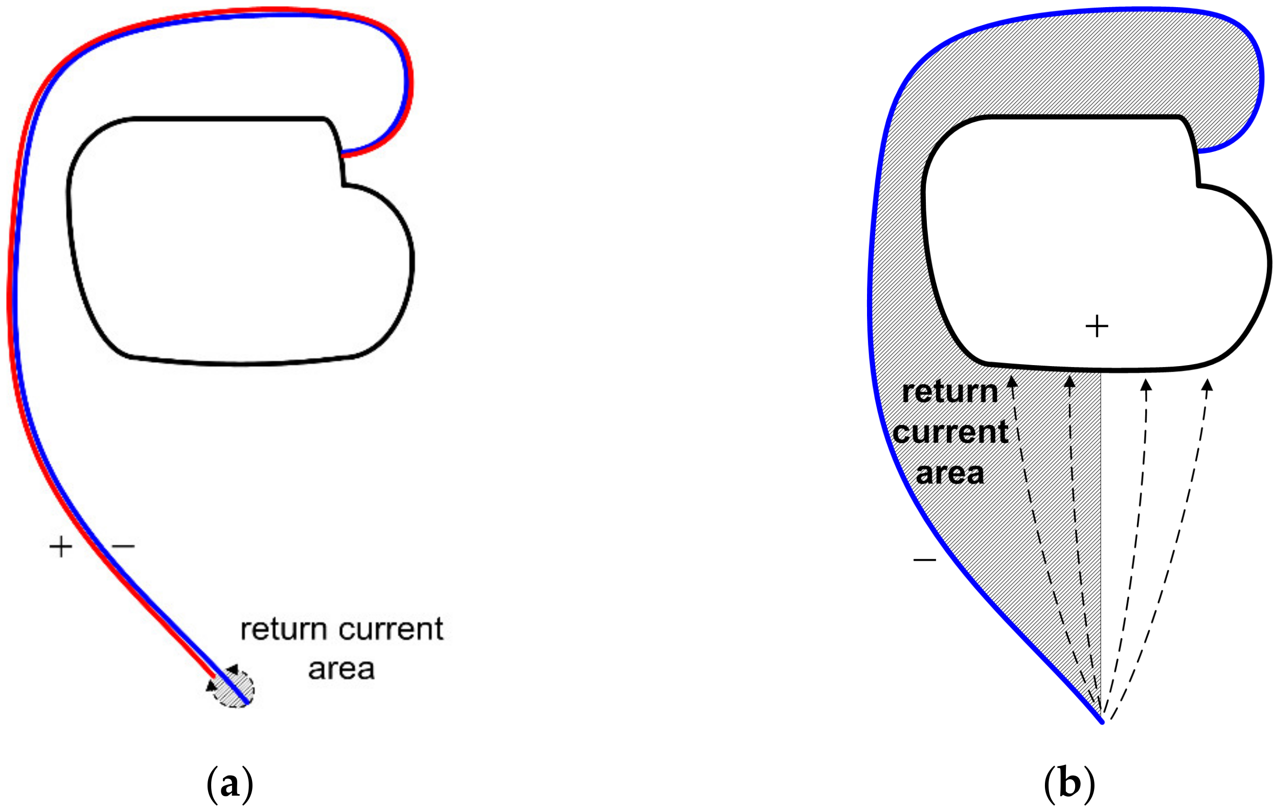
• Tip-to-ring distance taken at the worst-case 20 mm of a typical range of 8 to 20 mm;
• Lead length of 50 cm in a semicircular fashion giving a total area of about 315 cm² considering actual implantation situations, giving an effective area for induction of 225 cm²; these values are very similar to those in the ISO 14117 [70], where a survey of X-ray images of real implantations is reported;
• With the 20 mm tip-to-ring separation, the area of the equivalent circular sector is 24 cm² (that is probably slightly overestimated), leading to a proportion between the exposed area of the bipolar case compared to the unipolar case of 11%, confirming the aforementioned order of magnitude of reduction of induction.

The results of the modeling in Ref. [67] show that the induced voltage in bipolar mode, as caused by an external electric field, is 6% (9.7 against 161.0 μV/(kV/m)) and 12.9% (22.9 against 178.2 μV/(kV/m)) of the unipolar voltage for the cases of the half-inserted and fully-inserted tip in the cardiac tissue.

It was instead remarked by McIvor et al. [65] that at the high frequency of emissions characteristic of some EAS systems, such as the magneto-acoustic ones, the behavior of unipolar and bipolar PM with the same settings is the same (Figure 5 in [65]), possibly because there other types of coupling (e.g., reduction of common mode rejection in bipolar mode at high frequency). This is however not commented in the EN 50,527 standards.

The protection at a higher frequency is considered for example for WPT systems in the ISO 19363 [71], sec. 10.4.4, that assuming an induction model with B-field applied to the 225 cm² area, establishes a limit of 15 μT for the WPT frequency interval of 79–90 kHz.

2.3. Interference to Hearing Aids

Hearing aids are quite diffused and are used in a variety of situations: from listening to a concert that requires the highest quality, but can be excluded from this analysis, to listening to a conversation, to announcements (e.g., at a station) and in particular to safety-relevant messages, such as evacuation instructions. The operating principle may be subdivided as:

• Audiofrequency induction loop systems (AFILSs);
• Modulation radio transmission systems, including digital radio solutions;
• Systems based on infra-red (IR) technology.

The most diffused and most exposed to interference from power systems and electrical equipment are the AFILS. Also, those based on radio transmission are potentially exposed to interference, but mostly caused by another radio transmitter in close proximity, and are not considered here. Hearing aids, like all electronic products, pass the EMC tests [72], consisting of immunity to electrostatic discharge and radiated RF e.m. field (namely addressing issues of disturbance from the use of wireless devices and mobiles). As said, the low-frequency range is not covered, except for a magnetic field test at mains frequency, carried out at an intensity of 3 A/m, much lower than the exposure limits.

The type of interference should be evaluated against a concept of quality (e.g., signal-to-noise ratio or margin with respect to the reference level) for the expected function. Besides nuisance, noise may cause also a lack of attention or even lead to the intentional switch off of the worn device to escape an annoying situation (with the consequential inability to hear important messages).

The AFILS operates with the transmission of signals from a diffusing loop to the worn device; the transmission occurs in the audio band by means of a magnetic field, thus is intrinsically exposed to disturbance originating from power systems and electrical equipment with harmonics and commutation byproducts occurring in the same band. In particular, interference may occur with windings (such as coils and transformers) and power lines without compensation between phases (e.g., due to poor layout or by construction). AFILS are used extensively onboard ferries and passenger ships for areas accessed by passengers, not characterized by significant electric power deployment. A station platform instead is affected by the magnetic emissions of the catenary or third rail circuit (returning farther away through the running rails). Recently AFILS are being deployed also on-board trains (such as the new “Fleet of the Future” of the Bay Area Rapid Transit [73] and Ampetronic project [74]), where disturbance may be due to cable lines, converters, and filter inductors in close proximity.

In general, the main fundamental alone is not able to cause significant interference, as its A-weighting is quite low (see quantitative description below in Section 3.3): people are not receptive to frequencies of 50/60 Hz that may leak just as an unpleasant low-level hum. As a note, the noise that can be heard from buzzing transformers is at twice the fundamental frequency (mainly caused by magnetostriction) and thus more audible.

3. Compliance Requirements, Limits, and Frequency Ranges

This section reports the compliance requirements in terms of measurement methods, limits and frequency ranges enforced by applicable standards. The intention is to have a clear overview of the mandatory elements, on which the assessment approaches and measurement methods of Section 4 are developed. For an overview of standards and progress regarding human exposure (but not interference to implanted devices and hearing aids) reference may be made to [44].

3.1. Human Exposure

For human exposure, there has been worldwide a general convergence to a compliance framework in line with ICNIRP guidelines. Interaction of the e.m. field with the human body is classified in a set of phenomena that we have reviewed in Section 2.1. The ICNIRP guidelines report and justify the reference levels for the external measurable field quantities; such values have been in turn adopted by the European Union directives [11,75] and by many other regulations and national codes. The ANSI-IEEE standards [37,38] are more permissive over the frequency interval of interest, even after the 2010 increase of the older ICNIRP 1998 RLs, having removed some initial overestimating assumptions. An overview of limits for the external quantities (RLs) is provided in Figure 3:

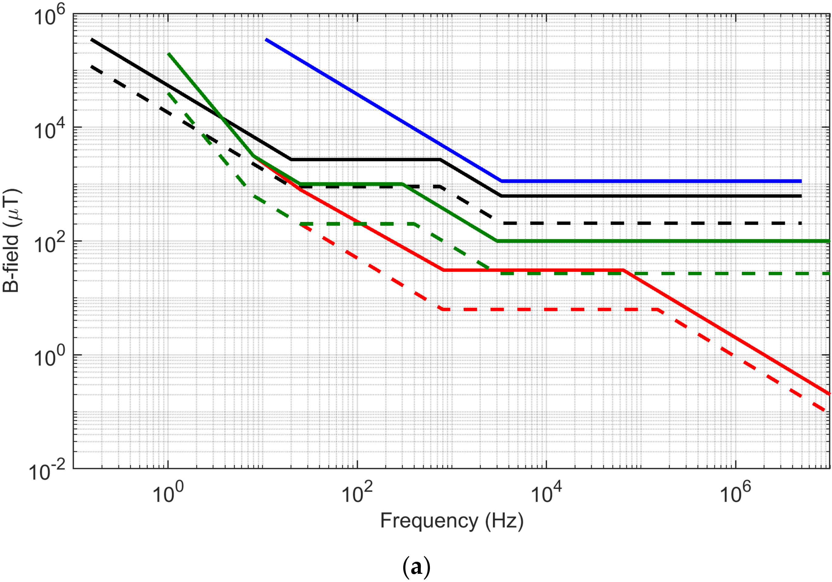
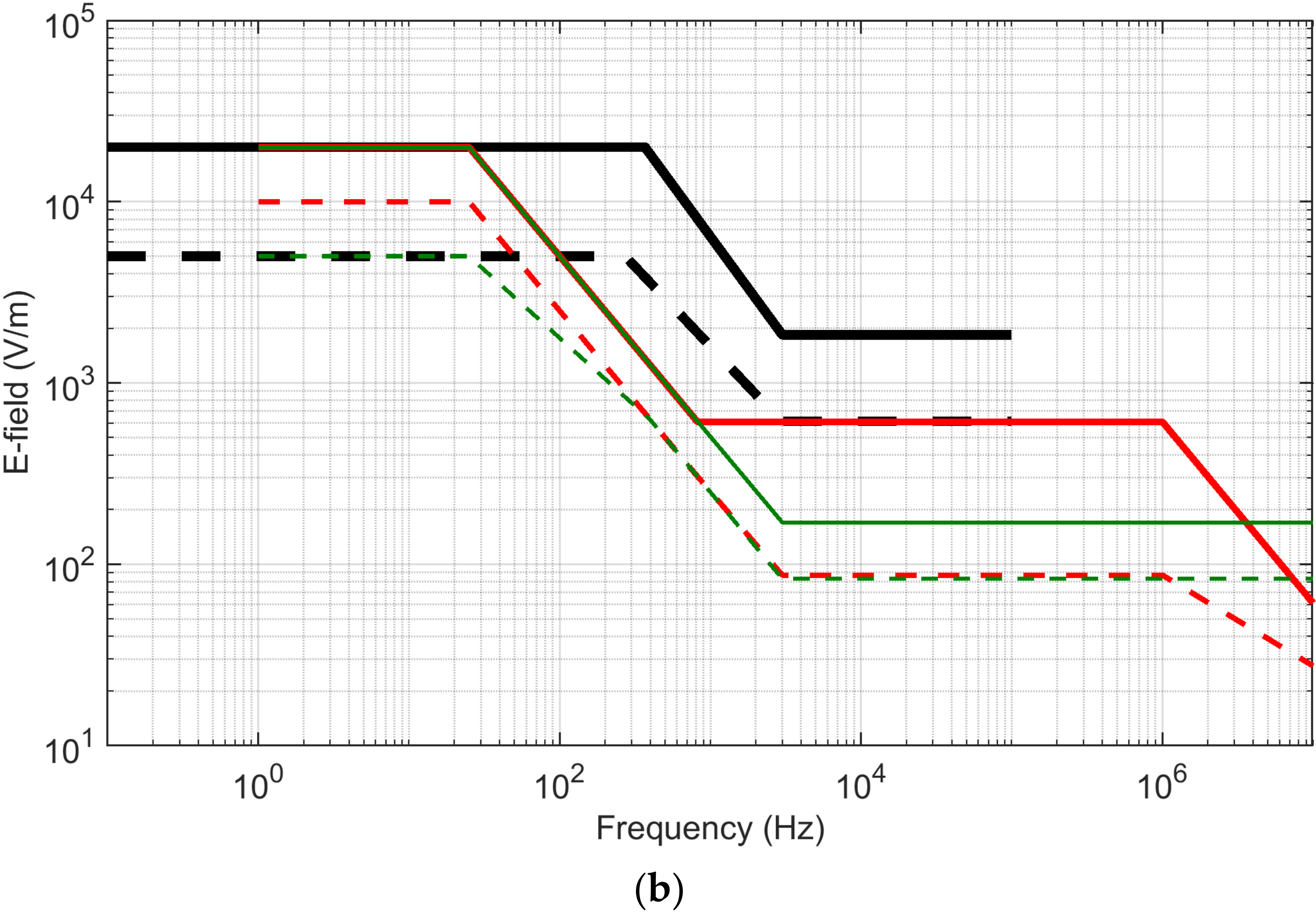
• Comparing the occupational and general public levels of the ICNIRP 1998 and 2010, the B-field RL has increased at high frequency by a factor of 3 and 4, respectively; conversely, for the E-field, the high-frequency values for occupational exposure only has seen a significant increase by about 3.5 times.
• IEEE includes de facto also a limit for the static field, whereas ICNIRP keeps it separate in a different guideline [5].
• IEEE does not report limits for whole-body exposure to the magnetic field (distinguishing three body parts, head, torso, and limbs), but does for the electric field. B-field exposure limits for occupational exposure have a margin of about 2 between head/torso (lower limits) and limbs (higher limits). Conversely, for general public exposure, the higher-margin is obtained by reducing the limits of exposure for head and torso, to less than 50% of the corresponding occupational values, but curiously the exposure limits for limbs are the same of the occupational scenarios.
• The IEEE RL values compared to ICNIRP are in general significantly higher, except for the low-frequency E-field where the two correspond.

As for the relevant frequency range over which, carrying out the assessment, some standards explicitly identify it for some classes of products. It is important to remark that sec. 5.2 of the IEC 62311 establishes the necessity of a 400 kHz extension when the highest internal frequency of equipment (for instance a switching frequency) is up to 10 kHz: for the mentioned EN 50500 [26] with converter switching occurring in the order of some kHz, a suitable frequency range for assessment would be then up to about 100 kHz.

Regarding contact current, the limits established by ICNIRP (for both the 1998 and 2010 versions) are quite low (1 and 0.5 mArms for occupational and general public exposure up to 2.5 kHz) and amount to the threshold of perception of the IEC 60479-1 [54]. Above 2.5 kHz, they increase linearly with frequency until 100 kHz, where they reach a limit value of 40 d 20 mA, held then constant up to 110 MHz.

3.1.1. Field Non-Uniformity, Field Gradient and Space Distribution of Points

Non-uniformity of field and field gradient (e.g., in case of very near sources) cause an uneven exposure of the subject, for which taking spatial averaging or maximum local field value can lead to two quite different results (the more conservative maximum might be preferable, but avoiding unnecessary overestimations is also welcome). The IEEE C95.3.1 [40] indicates two different approaches: for E-field exposure an average over the whole body is considered and compared to whole-body RLs (shown in Figure 3); for exposure to a magnetic field, the maximum local field value should be considered and compared to the relevant RLs (see Figure 3).

The measurement distance is quite a relevant parameter, especially for electrical equipment and tools that can be worn or are in close contact with the user: the IEC 61786-2 [76] in its Annex B lists distance requirements of various standards, including IEC 62110 [77], IEC 62311 [78], IEC 62597 [28] (EN 50500 [26]). The attention is focused on the distribution of points along the exposed body and the assumptions of the geometry of exposure and the relative source-person distance. They are reported in

Table 3. Overview of requirements for relative source-person distance and height above ground.

Standard	Distance from Source [m]	Height above Ground [m]
IEC 62110 [77] (AC power systems)	— 0.2 (1)	1 0.5, 1.0, 1.5
IEC 62597 [28] (2) (Rolling stock)	0.3	1.0, 1.5 (wrk in rsk) 0.3, 1.0, 1.5 (pub in rsk) 0.5, 1.5, 2.5 (wrk/pub out rsk) 0.5, 1.0, 1.5 (platforms)
IEC 62493 [79] (Lighting)	0.5–2.0 (3)	—
ISO 19363 [71] (4) (WPT)	0.2	up to height of vehicle three points midway on seat, back, and headrest
IEC 62905 [80] (WPT)	0.2	0.5, 1.0, 1.5

Notes: ⁽¹⁾ three-point measurement is for arithmetic body averaging; an “average exposure level” is also possible, that requires samples every 5 cm over the whole body volume (quite demanding); single point measurements are used in place of the average exposure level (assuming a uniform field) without specific distance requirement from the source; ⁽²⁾ meaning of abbreviations; “wrk” = workers, “pub” = public, “in rsk” = inside rolling stock, “out rsk” = outside rolling stock; ⁽³⁾ distance from lighting equipment depends on the installation and use (street light, bus light, etc.); ⁽⁴⁾ distance is specified from the external enclosure of the WPT vehicle for area 2, both for human exposure and interference to IMDs; the height above ground is up to the vehicle height; for interference to IMDs a grid of 7.5-cm spaced points is specified.

.

The EN 62110 covers human exposure in relation to AC power systems and focuses on emissions from overhead power lines, and at a lesser extent from cable lines and other power apparatus: a single-point measurement is indicated for uniform field situations and a three-point measurement (0.5, 1.0, 1.5 m above floor/ground along the vertical axis of a standing body) otherwise. It may be commented that a uniform field assumption should be corroborated by measurements, namely along three points as a minimum to calculate the gradient, for which a criterion is not given. Practical guides may give the indication to this aim of a maximum deviation of 10 or 20% of each point with respect to the average. As a matter of fact, the single-point measurement is never really applicable (Annex C of the EN 62110 discusses various geometries of exposure and related arrangements).

There are quite a few examples of significant gradients, especially in the case of electric vehicles and transportation systems with power systems and cabling located close to passenger seats and areas. In [81] the WPT system is shown to be characterized by a change of magnetic field intensity of more than 20 dB (an order of magnitude, from about 1 to 0.1 μT) across about 20 cm in the intermediate cross-section of an ideal vehicle with a steel frame at 85 kHz (resulting for the analyzed case in a compliant situation inside the vehicle for both the steel and aluminum frames). In [16] the calculated exposure for a dynamic WPT shows a difference of 20 μT and 800 μT across 10 cm in the horizontal direction for the cases of the WPT receiver mounted in the center and in the rear of the vehicle, respectively. The problem of the lateral gradient around power lines, both overhead and buried, is also well-known [8,9,10,76].

In general, for non-uniform fields, there are various methods that can be applied straightforwardly to measurements or may require some deal of modeling and calculation as additional support [78,80,82]: spatial averaging and local exposure, coupling factor, and generic gradient source model.

Spatial Averaging and Local Exposure

Taking the maximum of the external field in the point of the body closest to the source would lead to a significant overestimation potentially classifying a compliant scenario as non-compliant. Conversely, just taking the average would not guarantee the protection of the part of the body subject to the largest field values. The average is calculated of the exposure levels points distributed along the exposed body (e.g., 0.5, 1.0, 1.5 m above ground) and compared to the RLs (or ERLs); as a matter of fact, this approach implies that the non-uniformity is negligible, or that the margin with respect to the RLs is such to consider non-uniformity non-influential.

Without recurring to a full-body model and related calculations, and limiting the assessment to measured field values only, the most exposed parts of the body might be treated separately. The standard IEC 62905 [80] considers this approach: if compliance cannot be demonstrated using spatially averaged values, two other methods should be used. The first is just limiting the assessment to the part of the body that within an electric vehicle for example is really exposed, such as limbs, which are characterized by different limits of exposure in some cases (as carried out in [83] for the exposure of the driver’s foot). The second consists of using the coupling factor, for which the actual conditions (frequency, distance, field distribution) must correspond to those assumed for the derivation of the used coupling factor.

Coupling Factor

This approach is used for exposure from small equipment and electrical appliances, but also for exposure inside electric vehicles, as well explained in the IEC 62905 [80], the IEC 62311 introduced the coupling factor k_c taking the maximum measured B-field value with the objective of estimating J_i and attempting a less conservative evaluation with respect to BRs (or DRLs); the IEC 62233 [82] then introduced a multiplicative factor with the ratio of limits (RL/BR), obtaining the coupling factor a_c that allows the assessment of compliance to BRs based on the compliance to RLs (easier because based on external quantities).

$$k_c=\frac{J_{i,\max }}{B_{\max }}\hspace{1em}\hspace{1em}{a}_c=k_c\frac{J_{i,\lim }}{B_{\lim }}=\frac{J_{i,\max }/J_{i,\lim }}{B_{\max }/B_{\lim }}$$

(4)

The idea of the coupling factor a is that of replacing a magnetic field source with an equivalent magnetic loop and then comparing it to the selected limits (e.g., ICNIRP or IEEE). The procedure of the IEC 62233 is outlined below:

• A series of measurements of the B-field with a small volume probe (3 cm²) are taken at small steps (e.g., 0.5 to 1 cm) until the measured B-field drops to 10% of the initial maximum value at a given distance r₁₀ (taken after having identified that position as a hot spot).
• The integral over the distance of the measured B values up to r₁₀ is taken and an equivalent coil with the same integral value is determined; pre-calculated values for various coil radii and distances are shown in Table C.1 of the IEC 62233;
• The factor k_c is then determined by complex modeling that takes into account body conductivity σ_b, besides the coil geometrical factors; pre-calculated values for 50 Hz and σ_b = 0.1 S/m are reported in Table C.2 of the IEC 62233 and they can be extrapolated to other scenarios linearly in frequency (f/(50 Hz)) and conductivity (σ_b/(0.1 S/m)).
• For each frequency, the coupling factor a_c is determined as the scaled version of k_c, namely multiplying it by B_lim/J_i,lim (i.e., RL/BR). The value of a_c is plotted in Figure C.5 of the IEC 62233 for a coil radius ranging between 10 and 100 mm and the resulting value is quite stable and insensitive to coil radius, provided that the distance is larger than the said maximum coil radius, namely 100 mm.

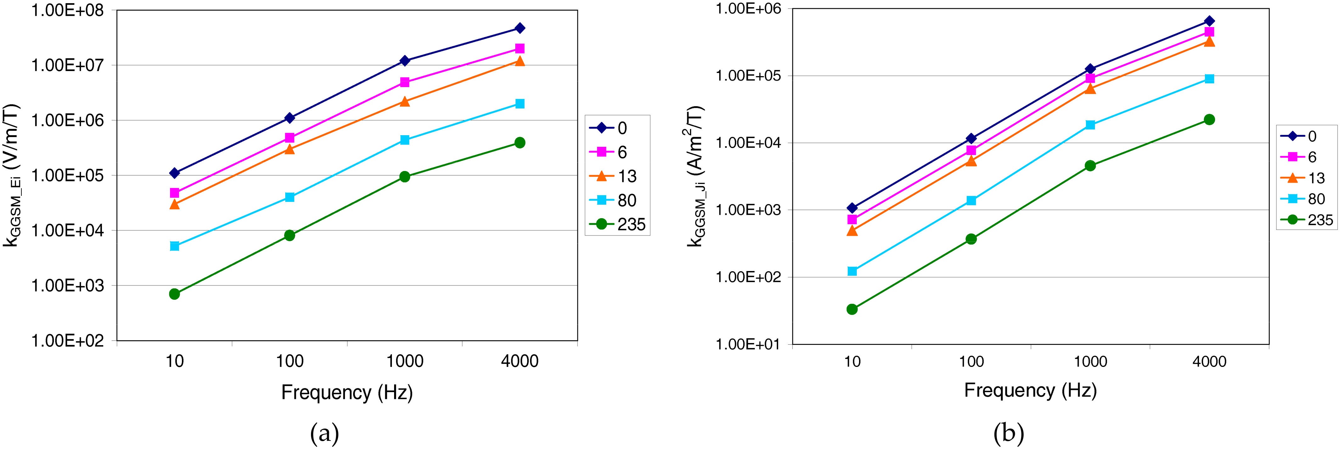
Generic Gradient Source Model (GGSM)

This method has been recently developed [80] specifically for exposure to WPT systems characterized by strong field gradients [84]. The standard does not clarify the method used to determine the GGSM values that relate the external B-field with the internal quantity E_i or J_i and that are reported for a range of frequency values and normalized B-field gradient g(B) = (dB/dp)/B, where p is a generic coordinate (see Figure 4). It is observed that the IEC 62905 refers to a “gradient field probe” as providing the B-field gradient but does not clarify which coordinate system is used (namely the gradient is taken along p = x, y, z separately or using a direction along which it is maximum).

A few points can be briefly commented on: The proportionality with frequency is almost linear but slightly more than that (within 10% for moderate g values). Considering the normalized gradient instead, there is no clear proportionality, ranging between linear and square root, and not so sensitive for the firsts two columns, passing from a situation of uniform field (g = 0) to a moderate gradient (g = 6). It is curious that the GGSM values for J_i are given with two significant digits contrasted whereas those for E_i with only one digit.

A step ahead is the use of coupling factors for other measurable external quantities, such as in particular the current in specific portions of an apparatus [14,84], particularly useful from two standpoints: it does not require a B-field measurement that can be easily related to the circuit currents using the Biot–Savart formulation and it is a precious indication of compliance and related margins already during design and assembly.

3.1.2. Multiple Spectrum Components at Different Frequencies

Simultaneous exposure to field components at different frequencies is commonplace in all real scenarios, although in some cases the approximation of one prevailing sinusoidal component may hold, such as for power systems with negligible distortion or a wireless charging system. The standard approach is applying the weighted sum of measured field components (see, e.g., sec. 4.2.2 of IEC 61786-2 [76]):

$$I_{f,E}={\displaystyle \sum _{f= 1 \mathrm{Hz}}^{10 \mathrm{MHz}}\frac{E(f)}{E_{RL}(f)}}\le 1\hspace{1em}{I}_{f,H}={\displaystyle \sum _{f= 1 \mathrm{Hz}}^{10 \mathrm{MHz}}\frac{H(f)}{H_{RL}(f)}}\le 1\hspace{1em}{I}_{f,B}={\displaystyle \sum _{f= 1 \mathrm{Hz}}^{10 \mathrm{MHz}}\frac{B(f)}{B_{RL}(f)}}\le 1$$

(5)

The IEEE C95.6 [38] indicates similar rules for multiple-frequency exposure and related summation, extending the summation down to 0 Hz:

$$K_{f,E}={\displaystyle \sum _{f= 0 \mathrm{Hz}}^{5 \mathrm{MHz}}\frac{E(f)}{E_{ERL}(f)}}\le 1\hspace{1em}{K}_{f,H}={\displaystyle \sum _{f= 0 \mathrm{Hz}}^{5 \mathrm{MHz}}\frac{H(f)}{H_{ERL}(f)}}\le 1\hspace{1em}{K}_{f,B}={\displaystyle \sum _{f= 0 \mathrm{Hz}}^{5 \mathrm{MHz}}\frac{B(f)}{B_{ERL}(f)}}\le 1$$

(6)

For both (5) and (6) the quantities at the numerator are rms values without phase information, the quantities at the denominator are the reference levels of ICNIRP or IEEE.

The ICNIRP and IEEE indexes resulting from summation are required to be less than unity. It is observed that the sum is carried out on the magnitudes of components only, resulting thus in overestimation. With the sum extended to include phase relationship, ideally, there is full correspondence with the “reverse response filter” (RRF in brief) time-domain method. The sum should be extended to the entire available frequency axis, but small differences are unavoidable due to several elements discussed in Section 3.1.3: accuracy of RRF transfer function and “smoothed” corners; RRF numeric implementation in terms of coefficient and sampling frequency; noise and some spectral leakage in the frequency domain implementation using the Fourier transform [85].

Criteria for inclusion/exclusion of spectral components from the summation are indicated in some standards:

• Sec. 5.5.1 of the IEC 62233 [82] and sec. 4.3 of the IEC 61786-2 [76] indicate 5% as the threshold for significance of harmonic content, where the percentage in the case of the IEC 61786-2 refers to the difference of exposure measured including and excluding harmonics;
• Sec. 5.3.2.1 of the EN 50500 [26] sets a significance threshold of 10% of the limit value;
• Sec. 4.2.2 of the IEEE C95.3.1 [40] instead indicates a 5% significance threshold referred to the fundamental or carrier (it is not clarified what happens for multiple sources and more than one fundamental).

To alleviate the overestimation of the “sum of magnitudes” criterion, an rms summation was proposed, as commented in the IEC 61786-2, sec. 4.2.5. An rms summation rule assumes that the distribution of the phases of the spectral components is arbitrary and random; components of a single source, however, may be highly correlated (such as the harmonics of a rectifier), so that the “real value” of the exposure may be closer to either the linear or the rms summation result depending on the number of independent sources and their characteristics of emission. The “weighted peak method” operating in the time domain instead gives always a correct result, provided that the RRF phase response is linear.

3.1.3. Non-Sinusoidal Field Waveforms

Although in principle all practical e.m. field waveforms are Fourier transformable, a frequency-domain approach is complicated by the large number of spectral components to include and the strong effect of their mutual phase relationship to preserve through the processing, besides the problems caused by spectral leakage. For these reasons, ICNIRP proposed in 2003 [2] a time-domain evaluation (later named the “weighted peak method”): this procedure was conceived in particular for EAS system emissions, featuring various types of impulsive patterns that challenged the traditional frequency-based method of assessment. Similarly, for highly dynamic environments, such as aboard trains [25] and electric vehicles [18,80,86], this time-domain approach is handier than the multi-frequency analysis discussed in Section 3.1.2. However, it does not allow discarding non-relevant spectrum components and noise, as shown above for the multi-frequency analysis.

The time-domain method exploits the duality between convolution in time and product in frequency domains and uses thus a filter with a frequency response corresponding to the inverse of the ICNIRP limit curve (that we have called “reverse response filter”, or RRF in brief), as shown in Figure 5.

The desired RRF transfer function is piecewise linear and follows a specific selected limit curve (such as the ICNIRP reference levels) and, when implemented using first-order blocks [2], is unavoidably smoothed at the corners joining the straight segments of the said limit curve. Besides the ideal implementation by the Laplace transfer function, the numeric implementation is best achieved by using an Infinite Impulse Response (IIR) digital filter architecture.

Using a low-order IIR implementation three points stand out regarding accuracy:

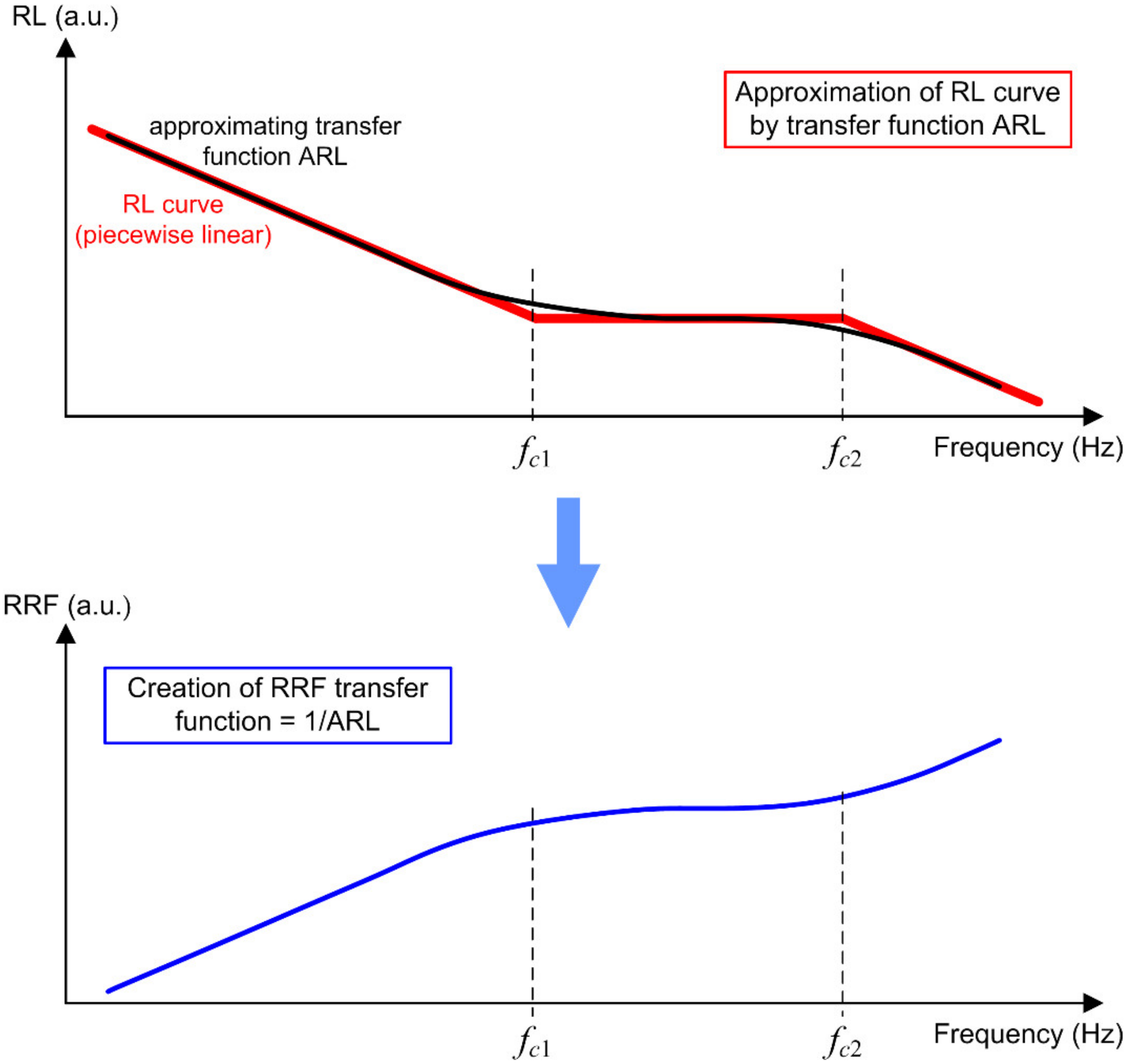
• Smoothing of corners, common also to analog implementations, for which there is an unavoidable loss of accuracy that can be evaluated as sketched in Figure 5;
• Phase response, that should not alter the phase relationship of the signal components; a zero-phase shift digital filter can always be implemented by exploiting the phase shift compensation occurring of the signal is passed through the filter twice, in the two time directions [85];
• Filter performance with respect to the adopted sampling frequency, compared to that of the original data samples: the RRF implementation in [25] revealed that to control filter response accuracy, the signal must be upsampled by about an order of magnitude, yet increasing correspondingly the computational burden.

A better approximation of the piecewise limit curve can be achieved by increasing the order of the filter at the expense of a more complex waveform.

The RRF output gives the so-called ICNIRP index, synthetically described as:

$$I_{t,E}=E(t)\ast RRF(t)\le 1\hspace{1em}{I}_{t,B}=B(t)\ast RRF(t)\le 1$$

(7)

having indicated with ∗ the convolution integral and RRF(t) the impulse response of the RRF filter.

Regarding calibration, it is observed that a sinusoidal tone is implicitly assumed also for instruments implementing the weighted peak method [87]: for the RRF transfer function phase errors, the response with complex waveforms would deviate from the correct one; this can be detected only using a more complex waveform, such as a square or triangular wave, or an impulse, as discussed in [88].

The IEEE C95.1 standard follows a different approach requiring at its sec. 4.2.3.3 that the rms of the measured field waveform complies with the ERLs for the unperturbed sinusoidal field. For magnetic field exposure, a requirement is added, consisting of the time derivative of B to be below a peak limit that is determined by the peak ERL at the characteristic frequency f_p = 1/(2t_p) multiplied by the pulsation (2π f_p). The quantity t_p is the peak duration (intended as the time between two zero crossings of the peak or for an exponential shape the time to reach 36.8% of the peak value.

$${\dot{B}}_{p,\lim }=\sqrt{2} (2\pi f_p) ERL(f_p)\hspace{1em}\hspace{1em}{f}_p=\frac{1}{2t_p}$$

(8)

3.1.4. Transients, Time Variability, and Time Averaging

The variable intensity of emissions may depend on variable operating conditions, as evident for an electric vehicle or rolling stock traveling under different speed regimes, but in general for all power systems, as power absorptions vary remarkably between day and night, and on a seasonal basis (including the effect of environmental conditions, such as temperature). A change of the fundamental current intensity is exemplified in Figure 3 of the IEC 61786-2.

As exposure is sensitive to the frequency distribution of components, variability may be caused also by:

• Changes to the spectrum of emissions (as in the case of a power drive or static power converter, exemplified for a French train in Figure 4 of the IEC 61786-2 and characterized in [89] for AC and DC rolling stock), or
• Transient waveforms, as caused by load steps, inrush, switch on/off and short circuits; it is generally agreed that major transients of this type should be discarded [82], but no criteria are given for example for repeated inrush events and switch on/off of loads.

This poses the issue of how to deal with transients and time-varying components, including non-stationarity. ICNIRP recommendation is that measured e.m. field “including transient or very short-term peak fields be regarded as instantaneous values which should not be time averaged.” Ideally, this is understandable and can be implemented if a straightforward time-domain evaluation is carried out, that, however, has to account for the averaging effect implicit in the first corner frequency of the RRF. Adopting the frequency-domain limit curves, instead, implies the use of the Fourier transform (e.g., FFT) and a consequential transformation window T of the time sampled signal, the lower the minimum frequency and frequency resolution, the longer its duration, and the implicit averaging over such window.

So, “instantaneous” is a concept that must be clarified under the conditions of use, for acquisition and processing and corresponds to the minimum observable frequency. For example, sec. 5.5.1 of the IEC 62233 [82] indicates to discard transients with duration less than 200 ms, exemplifying them as switching transients.

Sec. B.2.1.2.5 of the IEEE C95.1 [39] is more accurate and considers the excitation of nerves and muscles, giving an upper bound of 200 ms satisfying all scenarios. For very low frequency with a period exceeding 200 ms a longer integration time would be advisable: a 10 s interval is to be used for frequencies below 0.1 Hz.

The problem of the stationarity time interval was discussed in [25], where two approaches were confronted: one based on the correlation function and one simply estimating the minimum T value by observing the consistency of results obtained with progressively shorter transformation windows T. Similarly, the impulsive emissions and their stationarity have been considered for conducted emissions from converters [31], with considerations on alternative methods of evaluation, extendable to exposure to an electromagnetic field.

3.1.5. Additivity of Exposure to Electric and Magnetic Fields

Both external electric and magnetic fields concur to the internal field E_i (or current density J_i) and their contribution should be in principle summed vectorially for each point in the tissue, as advised in the ICNIRP 2010 itself [3], but then not implemented within the same guideline that reports as a matter of fact two separate relationships for exposure to the electric and magnetic field, each with its own unity limit for the summation (shown above in Section 3.1.2 and Section 3.1.3 for frequency and time domain). The IEEE C95.1, sec. B.2.1.10.3, clarifies that the contribution of the electric and magnetic field should be considered separately, and not additively, because their effect is maximized in different body regions (torso and ankles for whole-body exposure to uniform magnetic and electric field, respectively). The result of an arithmetic sum of the two terms calculated separately for their maximum E_i value is considered “very infrequent” by ICNIRP.

It is nevertheless true that there are cases of electric and magnetic field exposure occurring in the same body region (as shown in Table 2), with non-negligible values for a significant range of the intensity of the source:

• A typical high-voltage OHL provides both electric and magnetic field, in the order of some kV/m and several tens of μT at ground level beneath the line, and considering “ICNIRP 2010” in Table 2 results in alike contributions of internal electric field E_i in the brain of 3–5 and 1–2 mV/m, respectively; considering instead the fetal body labeled as “Dimbylow 2007”, the resulting values are about 2–4 and 0.5–1 mV/m; the contributions are clearly located in the same body region, the brain, and are commensurable, and should be summed together;
• For a different source that is prevalently magnetic (such as an MV/LV power transformer) at about 5–10 μT with a marginal electric field of some hundreds V/m, the previous contributions become 0.3–0.5 and 1–2 mV/m and 0.2–0.4 and 0.5–1 mV/m, resulting again in two alike terms, this time with prevalence of magnetic field induction, again in the same body region.

In general, assuming that the source of electric and magnetic field is the same (as under an OHL) and that the two vectors have the same frequency, the resulting internal field E_i components (E_i,E and E_i,H) are almost orthogonal by the respective coupling principles and an rms summation of the ICNIRP indexes would be closer to the exact result than the arithmetic sum of intensities.

3.2. Interference to Implantable Devices

There have been reported episodes of electromagnetic interference even with low-intensity static magnetic fields, affecting the operation of pacemakers (particularly those using magnetic switches) and other types of IMDs, including cardiac defibrillators, infusion pumps, neuromuscular and neurostimulators, and electronic prosthetic devices.

Many IMDs also contain ferromagnetic materials exposing them to the action of force and torque in a static magnetic field, causing movement and potentially dislocation. It may be observed, however, that most modern implants are not ferromagnetic. Based on studies performed to date, ICNIRP says “there is no evidence that static magnetic fields at or below the level of 0.5 mT would exert sufficient forces or torques on these devices to create a health hazard”. This sentence led to the inclusion of the 0.5 mT in the workers’ EU Directive [11], reducing the 1 mT limit indicated in the pacemaker EN 45502-2-1 standard. This 0.5 mT appears way too conservative, as it is orders of magnitude smaller than the field intensity discussed in Section 2.1.1 for mechanical interaction; rather, there were pacemakers with magnetic mechanical switches, that possibly justified this caution, although they are usually activated by a magnet positioned at a very short distance on the person’s chest.

PMs, ICDs, CRTs, and other IMDs are covered by a range of CENELEC [90,91,92,93] and ISO [70,94,95,96,97,98,99] standards for what regards electromagnetic compatibility (EMC) and interference; they are grouped in the following, discussing the type of immunity tests for qualification of products and the information available to provide to the assessment of exposure. New CENELEC standards [68,69,100] then address exposure of PMs, ICDs, and neurostimulators at the workplace, where higher intensity and a more extended frequency range is expected compared to domestic and general public exposure.

3.2.1. Pacemakers (PMs), Implantable Cardioverter Defibrillators (ICDs,) and Cardiac Resynchronization Therapy Devices (CRTs)

Pacemakers are covered by the EN 45502-2-1 [91] and ISO 14708-2 [95]. For what not explicitly specified in terms of EMC tests and criteria in the EN 45502-2-1, the EN 45502-1 generic standard should be used, which refers to an electromagnetic environment in line with the EU Dir. 519/1999 [75]. This clearly has pushed in the successive years the assessment of the exposure at the workplace, which is characterized by higher allowed field intensity in the order of a factor of 5. This has been concretized in the mentioned EN 50527 standards [68,69].

The EN 45502-2-1 and ISO 14117 [70] (recalled by the ISO 14708-2) divide the criteria in “induced lead current” (current erroneously delivered to the patient through the leads), “alteration of therapeutic behavior” (implying an alteration of cardiac signal sensing caused by the applied disturbance) and “persistent malfunction” (damage or malfunction persisting after the disturbance has ceased). The two latter criteria from an EMC point of view can be classified as: criterion A, with normal operation unaffected by the disturbance; criterion B, as a temporary malfunction that restore autonomously after the disturbance is finished, or criterion C, which needs some kind of intervention to restore normal operation, such as a manual reset, or ends up in a permanent malfunction that needs repair, or reprogramming. For criterion A and criteria B/C, respectively, the test levels differ significantly in the lower frequency range.

The disturbance is applied as a conducted signal through a test jig called “tissue equivalent interface” (intended for bipolar mode as a common-mode signal, the test differential signal being 10% of it) or as an electromagnetic field. The applied tests are:

• (T1.1) protection from the mis-reception of cardiac signals due to EMI, guaranteeing that the pacemaker provides its signals unaltered: square-wave modulated test signal (100 ms on, 600 ms off) with three quite extended frequency ranges (16.6 Hz to 150 kHz, 150 kHz to 10 MHz and 10 MHz to 450 MHz) and correspondingly amplitude ranging between 2–900 mV_pp, 0.9–10 V_pp, and 10 V_pp for the three frequency ranges); above 150 kHz the signal is amplitude modulated with a modulation depth of 95% at alternating intervals of 100 ms on, 600 ms off.
• (T1.2) extension of protection from mis-reception for the frequency interval 450–3000 MHz either by verification of the presence of feed-through filter for all leads going through the enclosure with a minimum insertion loss of 30 dB or by applying a test in line with the AAMI PC69 standard.
• (T1.3) protection from persisting malfunction with a test signal consisting of a swept sinusoid between 16.6 Hz and 140 kHz of 1 V_pp amplitude, increased proportionally to a frequency above 20 kHz (so that at 140 kHz it is 7 V_pp); when considering malfunction the tests signal is not square-wave modulated.
• (T1.4) protection from temporary malfunction during tests with a signal consisting of a sinusoid with frequency stepped between 16.6 Hz and 167 kHz and slowly increasing its amplitude from 0 to 1 V_pp at each frequency point.

As for the application of electromagnetic field, rather than a conducted test signal, the EN 45502-2-1 requires:

• (T2.1) a total immunity to a static field of 1 mT (criterion A) and protection from malfunction after application of a 10 mT intensity (criterion B).
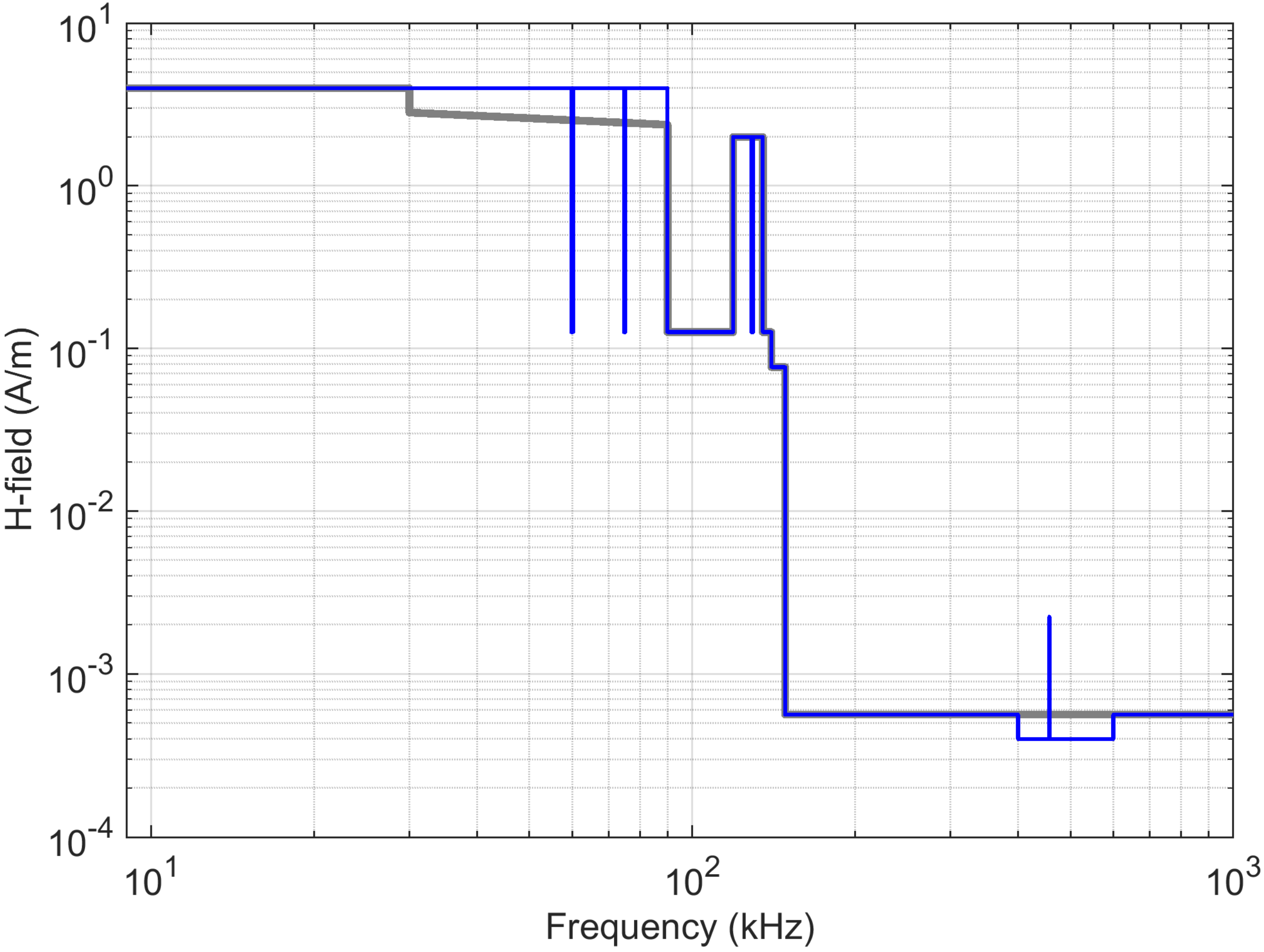
• (T2.2) protection from malfunction after application of a magnetic field at variable frequency, ranging from 1 kHz to 140 kHz and intensity of 150 A/m up to 100 kHz (linearly decreased between 100 and 140 kHz).

The ISO 14708-2 for EMC refers fully to the ISO 14117, which takes up the tests of the EN 45502-2-1 with some changes and in particular making the tests plan and criteria more clear:

• Upper-frequency limit for test T1.1 reduced to 385 MHz from 450 MHz;
• Test T1.2 modified as optional characterization in the range 385 to 3000 MHz, but the tests procedure is described in detail;
• For the immunity to static magnetic fields (test T2.1), the protection from malfunction is extended to 50 mT.

Implantable defibrillators are covered by the EN 45502-2-2 [92] and ISO 14708-6 [98] that for EMC refers fully to the ISO 14117 [70], that covers also CRT devices (both with pacing, -P, and defibrillator, -D, function). We see in the following the differences with respect to the EMC tests for pacemakers discussed above.

An often debated point is particularly important for the assessment of the protection of IMDs when the results of the human exposure assessment are available: if the ICNIRP 2010 RLs or IEEE C95.1 ERLs can guarantee the presumption of protection for the general public or occupational environments. This is discussed in the Annex M of the ISO 14117, whose results are reported in Figure 6 after some reworking. Since the coupling of the external E-field at low frequency occurs due to the induced current in the body J_i and is subject to variability (see Section 2.1), the ISO 14117 has estimated the coupling of the external B-field considering the values of the equivalent area of the PM/ICD leads (end of Section 2.2). A significant element pointed out by the ISO 14117 is the external field frequency being below or above the analog input low-pass filter of PMs, IMDs, and CRTs: a cutoff frequency of 1 kHz is considered and particular care to external field frequency around or below is recommended.

There are also some in situ studies that corroborate the identified grey areas for what regards the presumption of compliance using the human exposure limits as reference.

An extensive study of interference to PMs in unipolar and bipolar mode [101] showed that unipolar mode is more exposed and resulted in interference episodes (atrial tachycardia, ventricular tachycardia, and mode switch) for levels of the magnetic field above and below general public RL: the most troublesome waveforms were the ramp and square wave, followed by the pulsed waveform and then by the sinusoidal. Sine-wave field caused interference only at moderately low frequency (between 25 and 60 Hz) and a significantly large intensity above 300 μT, but below occupational RL. In general, looking at Table 3 in [101], interference from the first three types of waveforms occurs at levels of 4.5 to 15 μT, so more than an order of magnitude below the thresholds for the sinusoidal signal; this is probably due to the significant high-frequency spectral content and/or to steep rising and falling edges, that are completely absent in a sinusoidal waveform, but waveform characteristics are not documented in detail. The most affected devices were the Boston Scientific labeled in the work [101] as B4, B5, and B6, and a St. Jude Medical device labeled as C2, often when programmed in unipolar sensing and/or pacing mode. Only in a few cases interference resulted in configurations with the PM and leads parallel to the magnetic field orientation, indicating, in this case, that the noise was picked up by the leads or by the PM body, but marginally by the return current area. The work concludes that the higher RL allowed by the ICIRP 2010 compared to the 1998 edition should be considered cautiously.

Napp et al. [102] report the results of an extensive verification of susceptibility of 110 implanted ICDs of various types (single chamber, dual chamber, 3-lead devices) subject to controlled magnetic and electric field of variable intensity. Although responses are different depending on models, resulting in atrial or ventricular disturbance of various entities, the summarizing graphs of Figure 5 in [102] confirm that at normal sensitivity there was no interference for levels below the ICNIRP 2010 limits (both general public and workers), whereas the IEEE limits do not guarantee such level of protection, resulting in 10 out of 110 EMI cases. The number of interference cases increases with higher ICD sensitivity, selected during tests between maximum and nominal (although nominal may be equal to the maximum if advised by the treating physician). Responses were almost similar for the short (1.5 s) and long (30 s) exposure.

3.2.2. Cochlear and Auditory Brainstem Implants

Cochlear and auditory brainstem implants are covered by the EN 45502-2-3 [93] and ISO 14708-7 [99]. The ISO 14708-7 reports specific tests for such devices without referring to the ISO 14117. Although there is a general agreement on the type of tests, there are significant differences with respect to the ISO 14117 for intensity and frequency range of the external electromagnetic field applied to the device: the static field immunity test is carried out at 50 mT for both criterion A and B; the immunity to AC magnetic field is specified as shown in

Table 4. Immunity to magnetic fields between 16.6 Hz and 10 MHz for cochlear and auditory brainstem implants.

Frequency Range	Criterion A Test Level	Criterion B Test Level	Modulation
16–40 Hz	240 A/m (301 μT)	340 A/m (427 μT)	CW sin.
50–100 Hz	210 Am (301 μT)	850 A/m (1068 μT)	CW sin.
200–400 Hz	210 A/m (301 μT)	540 A/m (678 μT)	CW sin.
0.5–3 kHz	30 A/m (37.7 μT)	106 A/m (133 μT)	CW sin.
4–9 kHz	30 A/m (37.7 μT)	106 A/m (133 μT)	CW sin.
10–150 kHz	30 A/m (37.7 μT)	106 A/m (133 μT)	1 kHz, PM
0.2–3 MHz	4 A/m (5.0 μT)	21 A/m (26.5 μT)	1 kHz, PM
4–10 MHz	2 A/m (2.5 μT)	21 A/m (26.5 μT)	1 kHz, PM

.

3.2.3. Neurostimulators

Neurostimulators are covered by the ISO 14708-3 [96] and are characterized by similar immunity tests: a 50 mT test level is indicated, with a criterion of functionality after the tests as per nominal characteristics; a magnetic field immunity test is also required, as detailed in

Table 5. Immunity to magnetic fields between 1 kHz and 150 kHz for neurostimulators.

Frequency Range	Criterion A Test Level	Modulation
1–3 kHz	84/f A/m (105.6/f μT)	2 Hz, AM 95%
3–150 kHz	28 Am (35 μT)	2 Hz, AM 95%

(wording in sec. 27.105.2 of the standard is such that a criterion A can be deduced).

By comparison with the test levels used above for cochlear systems, the different test characteristics are apparent, although for the considered frequency range the applied intensity for criterion A is larger for the neurostimulators.

3.2.4. Circulatory Support Devices

Circulatory support devices are specifically covered by the ISO 14708-5 [97] and share a similar approach to the previous ones, although with some differences: the 50 mT is identical to the previous ones; the magnetic field immunity test is detailed in

Table 6. Immunity to magnetic field between 1 kHz and 140 kHz for circulatory support devices.

Frequency Range	Criterion A Test Level	Modulation
1–100 kHz	150 A/m (188.4/f μT)	CW sin.
100–140 kHz	15,000/f A/m (18.84/f mT)	CW sin.

and is strangely not subject to any modulation (so that a sinusoidal continuous wave should be assumed).

3.2.5. Occupational Exposure of IMDs

The EN 50527 standards [68,69,100] have been issued recently following the developed normative framework for occupational exposure (with the ICNIRP 2010 [3] and the EU Dir. 2013/35 [11]) and the identification of responsibilities for the employer regarding health and safety at the workplace. The EN 50527-1 sets the general framework, while the EN 50527-2-1 [68] and -2-2 [69] deal specifically with pacemakers and ICDs that may be considered the most commonplace among IMDs; the EN 50527-2-3 [100] for neurostimulators is still in the status of draft.

3.2.6. Conclusions and General Framework

The various EMC tests and test levels that characterize commercial devices have been presented and discussed, in order to derive a picture of the expected immunity especially compared to human exposure limits, that are more accessible and mandatory by law and represent thus the first reference.

The technological and normative progress and the consequential improved immunity and robustness to external e.m. influences apply to new products; it is nevertheless important to guarantee protection for the many older models that are still in use. On this, in the absence of a precise and complete normative framework for the 1980s and 1990s, the published findings represent still a valuable source of information to fill such gaps.

It is observed that in many cases reported in the literature malfunctions of PMs and ICDs occurred at power frequency magnetic field intensity slightly above the ICNIRP reference level of the general public at that time (100 μT at 50 Hz), leading to conclude that compliance for human exposure gave a margin fro what regards interference to PM and ICD. However, the reference level has been increased to 200 μT with the ICNIRP 2010 and occupational levels are larger, indicating that in both cases there might be interference, as they are above the immunity test level as per EMC product standards [91,92,95,96].

3.3. Interference to Hearing Aids

Measurements must be carried out with a magnetic field probe with the axis of one coil (or equivalently magnetic field sensor) aligned vertically, as the axis of the AFILS transmitting loop. Measurement positions should be selected randomly but shall correspond to the height above ground of the hearing aid for a standing (1.7 m) or sitting (1.2 m) person. Special seating requirements, unusual positions, and the influence of metallic objects nearby should be considered. The meter attached to the probe is required to have the following characteristics [12]:

• Frequency response flat within 1 dB between 50 Hz and 10 kHz, falling with at least 6 dB/octave at the boundaries;
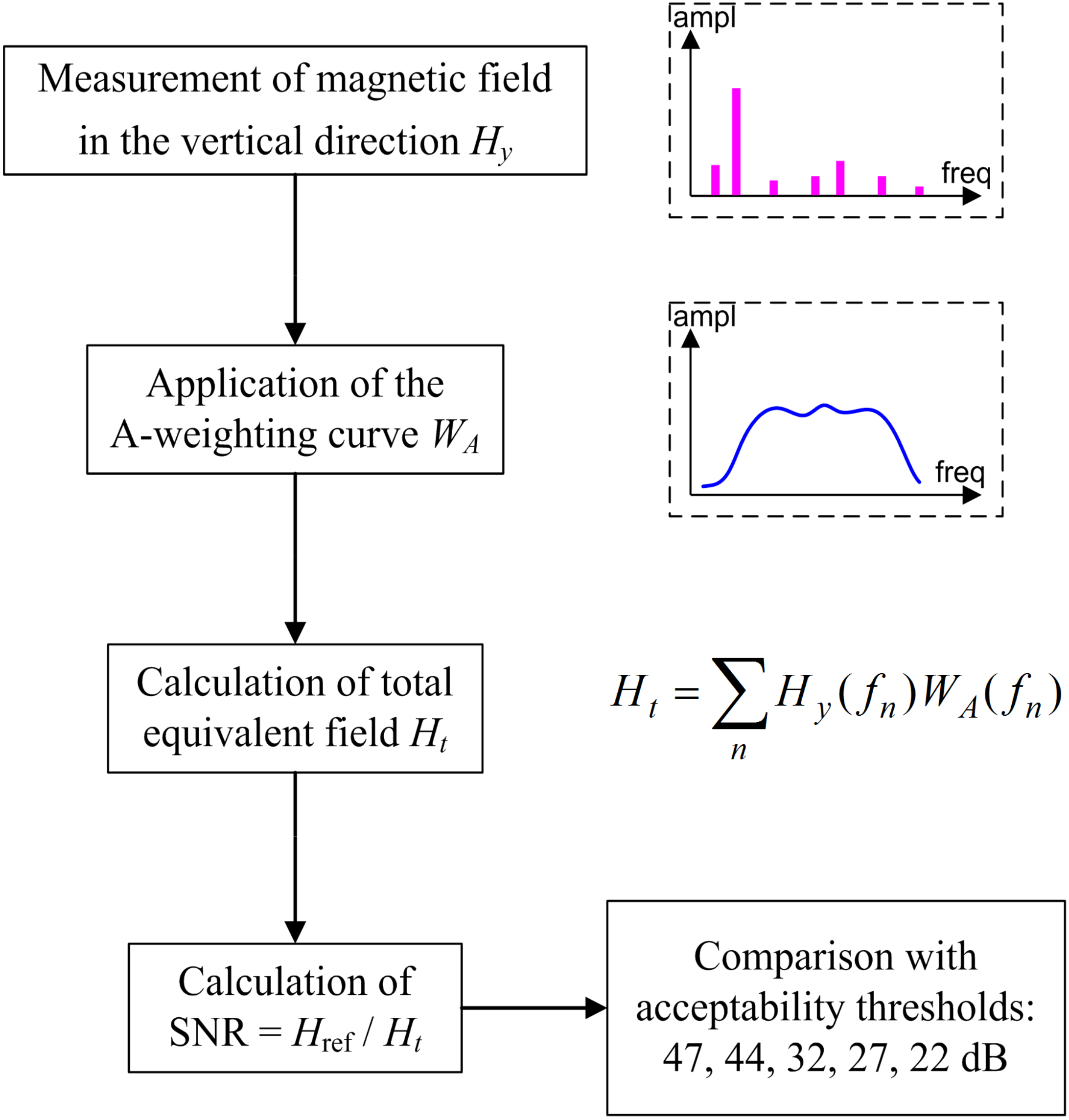
• Frequency response in A-weighted mode to conform between 100 Hz and 5 kHz “to Class 2 m specification in EN 61672-1 [103].”

The reference to the EN 61672-1 is in reality for integral meters providing an rms weighted reading. It is more profitable, considering the concomitant exigency of assessment of compliance to human exposure and IMD limits, to use a general-purpose magnetic field measuring system, followed by post-processing software. The software shall indeed be compliant in terms of uncertainty and frequency response.

The noise affecting the system is quantified as magnetic field intensity in the vertical axis weighted by a response curve simulating the sensitivity of the human ear (A-weighting curve) and compared to a reference magnetic field level used by the AFILS loop to transmit to the worn devices. This reference level H_ref is for example 0.4 A/m for the IEC 60118-4 [12] and 1 A/m for the Australian standard AS 1428.5 [13].

The target signal-to-noise ratio (SNR) in the EN 60118-4 is 47 dB. In cases where communication takes priority over aesthetic considerations, a higher magnetic noise level may be tolerated with a minimum SNR of 32 dB.

The EN 60118-4 allows a further relaxation to 22 dB if “the magnetic noise has no significant undesirable tonal quality or is mostly at low frequencies”. It is apparent that no better specified “tonal quality” and “low frequency” terms are subject to interpretation and that the simple reference to the EN 60118-4 is not sufficient to define a guaranteed requirement for the SNR, with a difference of 18 times between the desired target of 47 dB and the allowed minimum of 22 dB.

The AS 1428.5 establishes 44 dB of SNR (quite close to the 47 dB of the IEC 60118-4 if the different values of H_ref are considered) and a reduction to 21 and 27 dB (SNR for maximum speech intensity), with more pragmatic and quantifiable conditions regarding the presence or absence of fast-acting compressor/automatic gain control (FAC/AGC) in the worn device. In reality, both levels are referred to as a 15 dB acceptable average SNR level, where the presence or absence of FAC/AGC allows for an adapting dynamic range of 12 and 6 dB, respectively, considering average speech and maximum magnetic noise.

Transient components are weighted by the averaging time that is specified for the evaluation of acoustic and related quantities, and should be used for the evaluation of the external magnetic field noise too: the IEC 60118-4 and AS 1428.5 specify 0.125 s, whereas the ANSI S3.22 [104] speaks of 0.5 s for the high-frequency averaging (HFA), although not specifically referring to the problem of external disturbance. This was discussed in sec. 3.1.4 where the similar 200 ms was instead a hard reference to distinguish transients to discard from the evaluation.

The standards do not report a procedure for assessment nor an approach to the quantification of uncertainty: considering a magnetic field measurement followed by some post-processing (application of weighting curve to a measured or calculated spectrum and comparison with a set of SNR limit values), what already discussed for human exposure and interference to IMDs can be transferred in terms of measurement criteria, precautions and influential factors, as further discussed in Section 4. However, a clear indication is missing of the quantification of noise power, for what concerns colored noise and coherent components, the latter is often considered in electronics as a distortion rather than noise, and the relative amplitude taken as the significance threshold for such spectral components.

4. Assessment and Instrumentation

This section focuses on instrumentation and post-processing algorithms to assess compliance to the respective limits for the three domains that we have identified: human exposure, IMDs, and hearing aids. As observed at the end of the previous section, limits are defined on similar frequency ranges for the three domains, although they then might need different post-processing: general-purpose probes and acquisition systems may be considered that suit the overall set of technical requirements; time-sampled data are then more flexibly post-processed with the right algorithms for each domain.

After a discussion of the metrological characteristics in terms of hardware and software for instrumentation, some considerations are added of specific requirements for human exposure, IMDs, and hearing aids.

4.1. Requirements for Instrumentation

The requirements for suitable instrumentation are discussed in the following with reference to the minimum requirements derived from standards. It is underlined that there are standards requiring compliance to some limit to be demonstrated by measurement that fail to specify in sufficient detail the performance requirements for the measurement system.

4.1.1. Frequency Range

The frequency range must be in agreement with the relevant requirements, defined as a minimum between 1 Hz and 100 kHz, and including DC. It is to be extended to 150 kHz to cover disturbance to IMDs (with immunity documented up to 150 kHz) and 400 kHz to cover the minimum frequency range of the IEC 62311 [78] for electrical/electronic equipment. Having considered IEEE and ICNIRP requirements up to 5 and 10 MHz, respectively, the frequency range should be further extended by as much. This last extension is quite challenging from a technical viewpoint if a full-time domain is required [105] and as a matter of fact commercial equipment addresses this farther frequency interval by rms broadband measurements. To avoid the separate measurement of the DC component, rather than a coil-based probe, Hall effect, and Giant Magneto Resistive (GMR) sensors may be used, that however hardly reach the 1 MHz limit. Also, a combination of Hall/GMR and coils is possible, necessitating equalization in the signal conditioning block to achieve a flat response.

The −3 dB maximum frequency defines also the rise time of the instrument and the ability to follow undistorted steep fronts and pulses, such as for switching waveforms and pulsed power loads [88,106].

4.1.2. Dynamic Range

The dynamic range is the ratio between the maximum L_max and minimum L_min values of the reading scale of the instrument, that shall bracket the expected range of measurable values; given a maximum and minimum reference levels (or limit values) RL_max and RL_min, a margin must be added above (for out of scale and full representation of critical situations) and below, at least to provide adequate resolution and accuracy.

The IEC 62905 advises a 1–200% range measured with respect to RLs, that however must be considered with three important points in mind: there are two RL profiles for occupational and the general public with a difference up to about a factor of 5; IEEE and ICNIRP indicate different RL profiles again with a difference that may be as much as 3 and in some cases 10; then each RL curve is not constant with frequency and has an intrinsic dynamic range (RL_min to RL_max) of about two orders of magnitude. Summing all it up it is easy to see that the IEC 62905 principle translates into a requirement of six orders of magnitude (120 dB), as it was pointed out in [105].

4.1.3. Triaxial Probe and Isotropy

Triaxial measurements are needed for human exposure and IMD interference, for a complete representation of the field orientation and intensity, whereas for hearing aids only the vertical axis is required. Whenever not explicitly different, evaluation of compliance to human exposure and IMD disturbance limits is carried out using the intensity of the 3D field vector.

A triaxial arrangement brings along a requirement of isotropy: in general, a 5% (or about 0.5 dB) maximum isotropy deviation is required [26], but IEC 61786-1 [87] indicates a more restrictive 3%. Anisotropy or isotropy deviation is loosely defined as the difference of one of the axes with respect to the other two, although it is not clarified if it is the maximum or the average difference, take with respect to the other two axes and in turn for each of the three aligned with a reference external field.

4.1.4. Linearity

The relevance of linearity for human exposure measurements, is that any distortion byproduct will cause additional harmonics of the real e.m. field components to appear, and they are relevant since their effect is amplified by the fact that the reference levels decrease with increasing frequency. Without going into the details of the causes of diminished linearity (due to the characteristics of the internal electronic circuits and e.m. field sensors), it may be said the data sampling and conversion units (analog-to-digital conversion) have a negligible contribution in the order of some tens of parts-per-million. The sensors and front-end interfacing analog electronics instead may have a non-negligible contribution, depending on several factors, the most relevant the range of the measured quantity, as in many cases specifications of linearity are done for the entire dynamic range of the instrument, that is rarely exploited.

Usually declared values are in the order of 0.5–1%, implying a consequential distortion of the same order, that becomes irrelevant if compared to RL values for the nearest harmonics of, e.g., order 2 to 5, for those standards adopting a significance threshold of 5 or 10% of the RL values, as discussed in Section 3.1.2.

4.1.5. Amplitude Accuracy, Response Flatness, and Uncertainty

Regarding the amplitude of measured components, two main requirements may be distinguished: amplitude accuracy and frequency response flatness.

Amplitude accuracy is affected by the entire measurement chain, whether the signal transmission and acquisition are internal or shared among separate devices. In the latter case, as typical of EMC measurements, cable attenuation and reflections at ports are additional terms to consider: whereas cable attenuation (as other attenuations) is to be accounted for its uncertainty after the systematic error has been compensated, reflection is usually accounted for as a pure uncertainty term, being variable as a function of cable length and frequency. However, reflections are not relevant in this context for the considered frequency range.

The relevance of the frequency response flatness comes out when performing measurements in the time domain, for example for later post-processing. Any deviation from the desired flatness can be corrected during post-processing by applying deconvolution to the so distorted signal, provided that the frequency response is known.

The amplitude of the quantities of interest (individual spectral components or weighted index) is characterized by its uncertainty, describing the effect of the measurement process and the resulting spread of measured samples due to random effects.

The terms concurring to the amplitude uncertainty for each of the three x, y, z channels are well described in the IEC 61786-1 [87]: response of each field-sensing device (e.g., coil, dipole, Hall effect, GMR, etc.) including the stability of supply and biasing circuits; gain of each channel through the signal conditioning circuits to the ADC (analog-to-digital converter); terms characterizing the ADC itself, such as quantization noise, linearity, and spurious components. Practically speaking, however, an instrument is calibrated as a whole with its declared amplitude uncertainty.

4.1.6. Impact of Uncertainty on Compliance

The question is simple: provided that the measurement results after post-processing show compliance to limits, how reliable is this statement, considering that all measurement results are affected by uncertainty?

For the influence of uncertainty on a statement of compliance four cases can be identified when comparing a measured value with a limit, and the value is characterized by a confidence interval and confidence level (the uncertainty associated with a coverage probability), as graphically shown in Figure 7.

When the uncertainty of the measured value u(x_m) is estimated (e.g., with a Type A or Type B approach) and the maximum permissible uncertainty for the assessment u_max is acquired, there are two scenarios:

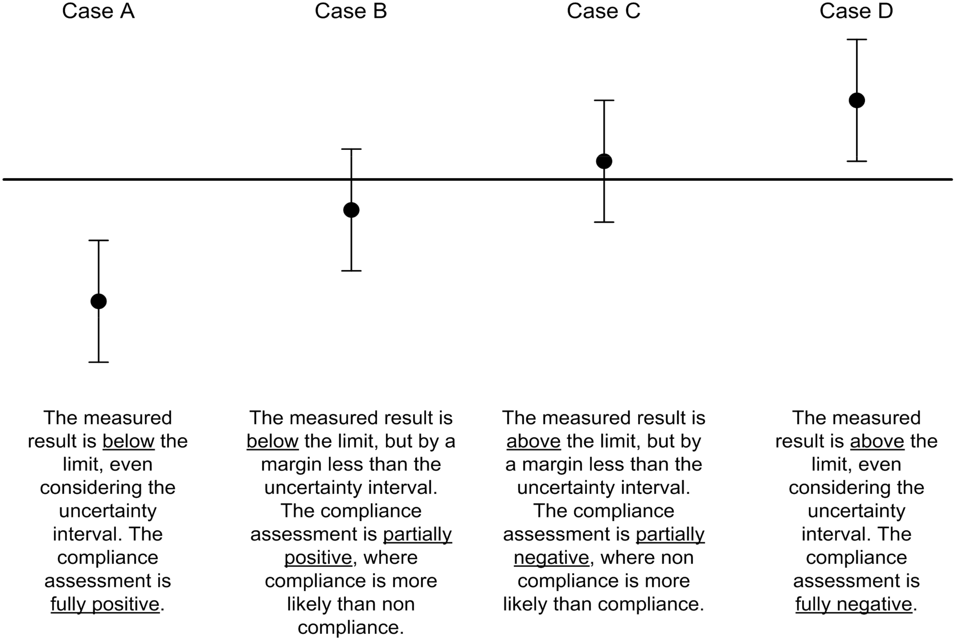
• If u(x_m) ≤ u_max then the measured value x_m can be compared directly with the limit x_lim (e.g., a reference level or the unity limit for the ICNIRP index).
• If u(x_m) > u_max then the actual uncertainty must be included, compared to the maximum uncertainty, resulting in a reduction of the limit by a so-called “penalty” that is shown at the denominator:

$$x_m\le \frac{x_{\lim }}{1-\frac{u_{\max }}{x_m}+\frac{u(x_m)}{x_m}}$$

(9)

The determination of the two uncertainty quantities (u(x_m) and u_max) is subject to some variability and interpretation, due to the following factors:

• There must be a standard specifying u_max for the specific application; in many cases, compliance is interpreted in an absolute sense, so without taking into consideration uncertainty and the probabilistic nature of measured values and the outcome of assessment (a good analysis of some cases is reported in [107]).
• The uncertainty u(x_m) may be related to the measurement setup and determined with a Type B approach, or associated to repeated measurements and determined with a Type A approach (including the variability of the operating conditions and the external noise sources, to cite the most evident exogenous influences, besides the instrumental uncertainty); this was discussed in detail for the measurement of electromagnetic field of large equipment and installations [108,109].

4.1.7. Factors Influencing Uncertainty and Uncertainty Budget

Complete analysis and evaluation of the uncertainty characterizing the assessment of exposure require a good understanding of both uncertainty in measurements and operating principles and characteristics of the instrumentation and of the assessed system (for field non-uniformity and variability of operating conditions).

Focusing on instrumentation, the uncertainty is evaluated for the measurement of a quantity. The combined uncertainty can be derived from an exhaustive list of factors contributing to uncertainty together with an estimate of their probability distribution as random variables and the sensitivity coefficients weighting the contribution of the single factor to the overall uncertainty [110,111,112]. Sensitivity coefficients c_i, assuming that the measured model function Y = f(X) is linear (or quasi-linear), where X_i are the input quantities affecting the measurement, are determined with the first-order partial derivatives as follows:

$$u(Y)=\sqrt{{\left[\frac{\partial f}{\partial X_1}u(X_1)\right]}^2+{\left[\frac{\partial f}{\partial X_2}u(X_2)\right]}^2+\cdots +{\left[\frac{\partial f}{\partial X_n}u(X_n)\right]}^2}=\sqrt{{\left[c_{1}u(X_n)\right]}^2+{\left[c_{2}u(X_n)\right]}^2+\cdots +{\left[c_{n}u(X_n)\right]}^2}$$

(10)

The assumption adopted so far is that the relevant input quantities are statistically independent and not correlated. The expression above (10) may be modified in a more complete form to take into account the correlation ρ_ij between input quantities X_i and X_j (correlation is a normalized adimensional quantity ranging between −1 and +1):

$$u(Y)=\sqrt{{\left[c_{1}u(X_1)\right]}^2+{\left[c_{2}u(X_2)\right]}^2+\cdots +{\left[c_{n}u(X_n)\right]}^2+2c_1{c}_2{\mathsf{\rho }}_{12}u(X_1)u(X_2)+\cdots +2c_i{c}_j{\mathsf{\rho }}_{ij}u(X_i)u(X_j)}$$

(11)

As a note, the factor of 2 is due to the symmetry of correlation for which ρ_ij = ρ_ji. The correlation coefficients may be calculated from the covariance between X_i and X_j, normalized by the product of the standard deviations. This calculation is carried out on the M realizations of each of the X_i and X_j quantities (indicated by small x):

$${\mathsf{\rho }}_{ij}=\frac{\mathrm{cov}(X_i,X_j)}{s(X_i) s(X_i)}=\frac{{\displaystyle \sum _{m=1}^M(x_{i,m}-{\overline{x}}_i)(x_{j,m}-{\overline{x}}_j)}}{\sqrt{{\displaystyle \sum _{m=1}^M{(x_{i,m}-{\overline{x}}_i)}^2}{\displaystyle \sum _{m=1}^M{(x_{j,m}-{\overline{x}}_j)}^2}}}$$

(12)

The estimate of correlation is quite complex, in that several samples are needed, with suitable, but practical, values of M in the order of 10 to 30.

Quite a complete list of these input quantities is exemplified in

Table 7. Elements contributing to uncertainty and indications for uncertainty budget [76,80,113,114,115,116].

Item	Source of Uncertainty	Distribution	Exemplified Tolerance/Range
1	Field amplitude (probe calibration uncertainty, possible use of flat gain; cannot be better than internal noise #10)	normal/ rectangular	often ambiguously specified as “accuracy”, typ. ±1% to ±3%
2	Field gradient (probe calibration uncertainty, spatially integrated gradient, see item #7 and #8)	normal	not available for all examined instruments
3	Probe anisotropy	rectangular (4)	declared often as ±5%, barely addressing compliance to standards
4	Probe linearity (relevant with large fundamental components)	rectangular	typ. ±1%, better for limited range
5	Probe frequency domain response (1)	rectangular	not fully specified, typ. ±1 dB at corner frequencies
6	Probe modulation response (e.g., with square pulse modulation)	rectangular	not available for all examined instruments
7	Probe spatial averaging (depends on probe area) (2)	rectangular	standard coil cross-sections of 100 and 3 cm2
8	Gradient uncertainty	rectangular	not available for all examined instruments
9	Parasitic E-field sensitivity (applicable to magnetic field probe)	rectangular	negligible for shielded construction
10	Internal noise (to evaluate, e.g., at 1–10% of the general public exposure; includes thermal and quantization noise)	normal	typ. 1% of full scale; higher for large dynamic ranges and in overload
11	Additional shaping, filtering, signal conditioning	rectangular/normal	If digital implementation, uncertainty negligible. If analog implementation, variable but up to 0.3–0.5%
12	Spatial positioning and moving error (3)	rectangular	site dependent, must be evaluated case by case
13	Repeatability (dispersion for repeated measurements)	normal	not available for all examined instruments; replaced by a statement of total uncertainty typ. ±5% to ±7%

Notes: ⁽¹⁾ Not uniquely defined: IEC 61786-2 relates it to insufficient coverage of harmonics and consequential reduced rms reading, that in reality is first a systematic error, but also depends on the characteristics of the signal not of the instrument; the operating frequency interval and its maximum extension instead determines the rise time of the instrument transient response that is relevant for pulsed and steep edge waveforms (converter switching, pulsed source, etc.). ⁽²⁾ Given an approximately circular coil, this is a characteristic parameter that may be subject to some amount of variability due to the non-circular shape and coil area uncertainty; for Hall effect and GMR the probe area is minimal and averaging is much reduced, but has a larger uncertainty, due to fabrication and mounting tolerance of semiconductor devices. ⁽³⁾ Automated measurement systems have sweeping probes with a speed constraint given by the probe transient response and the field gradient (local variability); more commonly the probe takes one measurement at a time and measurement error corresponds to a positioning error. ⁽⁴⁾ The word “rectangular” indicates the uniform distribution.

, having considered the IEC 62905 [80] and IEEE Std. 644 [112], and added in the last column some information from existing instrumentation and calibration procedures. Such examples for human exposure and assessment of interference to IMDs are common to some extent to higher frequency EMC measurements, for which some other considerations may be found in [113].

Instruments considered in this work [114,115,116] are all medium to high range instruments ensuring compliance to standard specifications we have reviewed so far and selected for illustrative purposes. There are others available at lower prices, that however provide lower performance, but do not prevent carrying out an assessment with larger uncertainty, that deserves also additional care especially for undocumented undesired responses and behavior. Listing of manufacturers or instruments’ models does not imply any form of endorsement.

By inspection of Table 7, it is apparent that even high-end instruments do not address all relevant requirements set forth by the considered standards [76,80,117], in particular those related to field gradient and probe spatial integration, that are of utmost importance in situations of field inhomogeneity and in quite recent applications, such as automotive and wireless power transfer [118,119].

4.2. Human Exposure Assessment

The preliminary phase of the assessment is the identification of individual sources and relevant operating conditions. The operating conditions then may be under control or not, and the characterizing quantities known with variable accuracy (e.g., load current measured by a panel meter). Taking several measurements and tagging them with the supposed operating conditions (e.g., value of the load current), the estimate of dispersion of the measured values for identical or different operating conditions, allows determining the stability of such operating conditions and the presence of other relevant factors affecting the measurement results.

The assessment of compliance may be carried out with increasing complexity by following the three steps highlighted in Figure 8: relevance of sources may be based on an initial assessment of the main characteristics, such as maximum power or current, that allows a first simplified assessment based on lack of relevance; then, the measurement of external quantities and comparison with reference levels can achieve the demonstration of compliance (although in some cases calculation with suitable models is acceptable); lasts, if compliance cannot be assessed for a range of reasons (e.g., too coarse measurements, exaggerated approximations and conservative assumptions, etc.), the basic restrictions must be considered, feeding the comparison with either measurements on a volunteer (J_i of whole body or limbs) or a phantom (J_i and E_i at all points), or extrapolation by using the coupling factor or GGSM.

The completeness and representativeness of the assessment highly depend on how the measurement positions and the operating conditions have been chosen and if they can be considered a worst-case picture of the exposure scenario. In some cases, when selected positions may influence the results (including uncertainty due to field gradient), thee relevant standards make a thorough specification, as for electric vehicles and the 3 positions at car seats of IEC 62905 and the 7 points on seat and console of the Chinese std. GB/T 37130, discussed in [84].

4.3. Implantable Medical Devices

The EN 50527 standards describe the assessment process beyond the technical elements characterizing the measurement and evaluation on which we have focused so far. Figure 2 of the EN 50527-2-2 and -2-3 includes the analysis of the characteristics of the activity of the employee, warnings for the specific equipment in use, and consultation with the physician. If additional investigations are deemed necessary, the standards discuss the possible investigations (clinical and non-clinical) and give an outline of the process.

If the assessment of compliance for IMDs is carried out by measuring the external field intensity and comparison with limits, there are no specific precautions other than those already reviewed for human exposure measurements and then those of Section 4.5 below. The assessment is in fact carried out with all the overestimating factors related to the geometry of induction and the characteristics of the body with the IMD.

If, however, it turns out that such margins would configure a non-compliant scenario for which control measures are not suitable nor convenient to implement, a more refined approach of determination of the real device exposure may be carried out. Besides clarifying the type of IMD and its constructive characteristics (brand/model, unipolar/bipolar, settings and susceptibility), and the specific implantation characteristics (location, length of leads, etc.), other relevant factors are the orientation and gradient of the field (as worst-case oriented uniform field is assumed), the exposed body characteristics (e.g., sex, weight, height) and geometry of exposure (posture, if sitting/standing, etc.). We have seen in fact that all such factors imply variability of results of the examined studies and limits and standardized procedures adopt maximum or reasonably large values. The reduction of overestimating assumptions, whenever reasonable and demonstrable, is a first viable approach to a refined assessment, tailored to the specific situation.

If agreement is not reached or results are not conclusive, a specific study of the response of the specific IMD in real conditions may be carried out: in this case an expert physician should be present to guarantee the safety of the person and to verify the behavior of the IMD with suitable instrumentation and interpretation of results.

4.4. Hearing Aids

The overall quantification procedure can be synthesized as in the flowchart of Figure 9, where, starting from the measurement of the H-field at selected frequency values f_n, the application of the A-weighting curve W_A (to apply at the f_n values), the application of the reference level H_ref (0.4 or 1 A/m depending on the use of thee IEC 60118-4 or AS 1428.5) and the calculation of the resulting signal-to-noise ratio SNR are clarified. The SNR value is then compared to the limit thresholds, having already discussed the conditions for application of the SNR limits.

4.5. General Measurement Precautions

Besides the compliance with the hardware and software requirements, reliable results are obtained when measurements are carried out correctly, using precautions that might depend on the characteristics of the source and space constraints.

One major point is the unwanted coupling of the probe with conductive parts nearby (including operator’s influence for high-impedance fields such as the low-frequency E-field). Similarly, unless clearly prescribed by the applied standard, a safe distance from the source itself should be maintained to avoid capacitive coupling. As already discussed, situations with significant field gradient should be annotated describing the way readings are taken and how the amount of gradient is estimated (although not explicitly prescribed by the applied standard).

A good practice is that of taking repeated measurements both as successive readings and separate measurements after repositioning the instrument and reproducing the desired system conditions, in order to check repeatability and stability of measurement conditions.

5. Conclusions

The work has considered the problem of human exposure and interference to IMDs, and by extension to hearing aids, in the context of modern power systems, that encompass, for example, power distribution, microgrids, power apparatus, electric transports. After demonstrating the variety of emissions affecting both the general public and workers, the attention has been focused on the mechanisms of interaction and the quantitative criteria that relate the external measurable quantities with the internal ones, characterizing the exposure or interference. This is particularly important to understand the standpoint of standardization committees and the possible evolution of limits, considering a significant development of standards and regulations, that concretizes in the production of more than 40 standards all inherent and analyzed throughout the work. The responsibility of the employer has recently received more attention, resulting in an attempt to clarify the technical elements and the approaches to the assessment.

Section 3 has considered the problem of identification of limits and requirements by discussing and confronting several standards, in particular, to clarify possibly ambiguous definitions, such as related to the processing in the frequency or time domain of acquired measurements, field uniformity, evaluation of transients, additivity of electric and magnetic field effects.

For some existing standards (such as for guideway transportation systems [26]) the extension of the frequency range would be advisable to chase new faster power conversion technology and in line with other similar applications [78,80]. In general, available instrumentation can cover a fairly wide frequency interval and amplitude dynamic range, if interchangeable probes are chosen wisely following well formulated and clear requirements. The exemplified instrumentation demonstrates that 400 kHz is a standard upper frequency chosen by the manufacturers to comply with many standards; possibly, for applications characterized by high-frequency content (smart converters, next-generation wireless power transfer, etc.) a frequency interval extended to 1 or a few MHz would be advisable (a rigorous approach against the most extended ICNIRP specification [3] would indicate 10 MHz).

For the assessment in the case of a non-uniform field some methods are available (coupling factor and generic gradient source model, GGSM) that have been derived for specific cases, such as for electric appliances or electric vehicles and wireless charging: their applicability to a wider range of systems as in modern microgrids and distributed generation should be further investigated, to facilitate the evaluation of exposure starting from the design phase.

The available high-level instrumentation is nowadays quite standardized to cover the most common requirements, but problems may arise for the extension to new standards and applications (including covering human exposure, interference to IMDs and hearing aids at the same time), as well as for a thorough demonstration of the assessment uncertainty, as shown in Section 4. The latter in fact is sometimes confused with and limited to the statement of the instrumental uncertainty (possibly lacking the characterization of the instrument with respect to field gradient conditions and response to transients), while setup uncertainty is not duly considered. A list has been drawn of relevant factors to consider using the most complete standards and exemplified referring to some well-known instruments. Nevertheless, such a list may be extended and customized for specific applications, taking into account the characteristics of the installation, system behavior, and interaction with humans (e.g., in terms of positioning and relative distance from sources).

References

1. ICNIRP. Guidelines for Limiting Exposure to Time-Varying Electric, Magnetic, and Electromagnetic Fields (up to 300 GHz). Health Phys. 1998, 75, 494–522. [Google Scholar]
2. ICNIRP. Guidance on Determining Compliance of Exposure to Pulsed Fields and Complex Non-Sinusoidal Waveforms below 100 kHz with ICNIRP Guidelines. Health Phys. 2003, 84, 383–387. [Google Scholar]
3. ICNIRP. Guidelines for Limiting Exposure to Time-Varying Electric and Magnetic Fields (1 Hz–100 kHz). Health Phys. 2010, 99, 818–836. [Google Scholar]
4. ICNIRP. Guidelines for Limiting Exposure to Electromagnetic Fields (100 kHz–300 GHz). Health Phys. 2020, 118, 483–524. [Google Scholar]
5. ICNIRP. Guidelines on Limits of Exposure to Static Magnetic Fields. Health Phys. 2009, 96, 504–514. [Google Scholar]
6. Salvan, A.; Ranucci, A.; Lagorio, S.; Magnani, C.; SETIL Research Group. Childhood Leukemia and 50 Hz Magnetic Fields: Findings from the Italian SETIL Case-Control Study. Int. J. Environ. Res. Public Health 2015, 12, 2184–2204. [Google Scholar] [CrossRef] [PubMed] [Green Version]
7. Gajšek, P.; Ravazzani, P.; Grellier, J.; Samaras, T.; Bakos, J.; Thuróczy, G. Review of Studies Concerning Electromagnetic Field (EMF) Exposure Assessment in Europe: Low Frequency Fields (50 Hz–100 kHz). Int. J. Environ. Res. Public Health 2016, 13, 875. [Google Scholar] [CrossRef] [PubMed] [Green Version]
8. Salceanu, A.; Paulet, M.V.; Neagu, C.D.; Bordeianu, D.F. On the coupling influence of the relative position of human trunk with respect to the overhead high-voltage power line. Acta IMEKO 2020, 9, 53–58. [Google Scholar] [CrossRef]
9. Ignatenko, I.V.; Vlasenko, S.A. Health assessment of the electrical contact-line connections in view of the operational traction load pattern of the electric rolling stock. In IOP Conference Series: Materials Science and Engineering; IOP Publishing: Bristol, UK, 2020; Volume 918, p. 012154. [Google Scholar] [CrossRef]
10. Safigianni, A.S.; Tsompanidou, C.G. Electric- and Magnetic-Field Measurements in an Outdoor Electric Power Substation. IEEE Trans. Power Deliv. 2008, 24, 38–42. [Google Scholar] [CrossRef]
11. EU Dir. 2013/35. Directive of the European Parliament of 26 June 2013 on the Minimum Health and Safety Requirements Regarding the Exposure of Workers to the Risks Arising from Physical Agents (Electromagnetic Fields) (20th Individual Directive within the Meaning of Article 16(1) of Directive 89/391/EEC) and Repealing Directive 2004/40/EC; European Union: Brussels, Belgium, 2013. [Google Scholar]
12. IEC 60118-4. Electroacoustics—Hearing Aids—Part 4: Induction-Loop Systems for Hearing Aid Purposes—System Performance Requirements; IEC: Geneva, Switzerland, 2015. [Google Scholar]
13. AS 1428.5. Design for Access and Mobility—Part 5: Communication for People Who are Deaf or Hearing Impaired; Australian Standards: Sidney, NSW, Australia, 2010; (reconfirmed 2016). [Google Scholar]
14. Hakuta, Y.; Watanabe, T.; Takenaka, T.; Ito, T.; Hirata, A. Safety Standard Compliance of Human Exposure From Vehicle Cables Using Coupling Factors in the Frequency Range of 0.3–400 kHz. IEEE Trans. Electromagn. Compat. 2021, 63, 313–318. [Google Scholar] [CrossRef]
15. Campi, T.; Cruciani, S.; Maradei, F.; Feliziani, M. Magnetic Field during Wireless Charging in an Electric Vehicle According to Standard SAE J2954. Energies 2019, 12, 1795. [Google Scholar] [CrossRef] [Green Version]
16. Cirimele, V.; Freschi, F.; Giaccone, L.; Pichon, L.; Repetto, M. Human Exposure Assessment in Dynamic Inductive Power Transfer for Automotive Applications. IEEE Trans. Magn. 2017, 53, 1–4. [Google Scholar] [CrossRef]
17. Ding, P.-P.; Bernard, L.; Pichon, L.; Razek, A. Evaluation of Electromagnetic Fields in Human Body Exposed to Wireless Inductive Charging System. IEEE Trans. Magn. 2014, 50, 1037–1040. [Google Scholar] [CrossRef]
18. Vassilev, A.; Ferber, A.; Wehrmann, C.; Pinaud, O.; Schilling, M.; Ruddle, A.R. Magnetic Field Exposure Assessment in Electric Vehicles. IEEE Trans. Electromagn. Compat. 2014, 57, 35–43. [Google Scholar] [CrossRef]
19. Christ, A.; Douglas, M.; Nadakuduti, J.; Kuster, N. Assessing Human Exposure to Electromagnetic Fields From Wireless Power Transmission Systems. Proc. IEEE 2013, 101, 1482–1493. [Google Scholar] [CrossRef]
20. Emadi, A.; Rajashekara, K.; Williamson, S.S.; Lukic, S. Topological Overview of Hybrid Electric and Fuel Cell Vehicular Power System Architectures and Configurations. IEEE Trans. Veh. Technol. 2005, 54, 763–770. [Google Scholar] [CrossRef]
21. EN 103 409. System Reference Document (SRdoc); Wireless Power Transmission (WPT) Systems for Electric Vehicles (EV) Operating in the Frequency Band 79–90 kHz; ETSI: Sophia Antipolis, France, 2016. [Google Scholar]
22. Celaya-Echarri, M.; Azpilicueta, L.; Lopez-Iturri, P.; Aguirre, E.; De Miguel-Bilbao, S.; Ramos, V.; Falcone, F. Spatial Characterization of Personal RF-EMF Exposure in Public Transportation Buses. IEEE Access 2019, 7, 33038–33054. [Google Scholar] [CrossRef]
23. Buyakova, N.; Zakaryukin, V.; Kryukov, A.; Lagunova, N. Electromagnetic safety of railway electrification systems under deicing. Energy Saf. Energy Econ. 2018, 5, 5–10. [Google Scholar] [CrossRef]
24. Halgamuge, M.N.; Abeyrathne, C.D.; Mendis, P. Measurement and analysis of electromagnetic fields from trams, trains and hybrid cars. Radiat. Prot. Dosim. 2010, 141, 255–268. [Google Scholar] [CrossRef]
25. Bellan, D.; Gaggelli, A.; Maradei, F.; Mariscotti, A.; Pignari, S. Time-Domain Measurement and Spectral Analysis of Nonstationary Low-Frequency Magnetic-Field Emissions on Board of Rolling Stock. IEEE Trans. Electromagn. Compat. 2004, 46, 12–23. [Google Scholar] [CrossRef]
26. EN 50500. Measurement Procedures of Magnetic Field Levels Generated by Electronic and Electrical Apparatus in the Railway Environment with Respect to Human Exposure; CENELEC: Brussels, Belgium, 2015. [Google Scholar]
27. Mariscotti, A.; Sandrolini, L. Review of models and measurement methods for compliance of electromagnetic emissions of electric machines and drives. Acta IMEKO 2021, 10, 162–173. [Google Scholar] [CrossRef]
28. IEC 62597. Measurement Procedures of Magnetic Field Levels Generated by Electronic and Electrical Apparatus in the Railway Environment with Respect to Human Exposure; IEC: Geneva, Switzerland, 2019. [Google Scholar]
29. EN 300 330. Short Range Devices (SRD);Radio Equipment in the Frequency Range 9 kHz to 25 MHz and Inductive Loop Systems in the Frequency Range 9 kHz to 30 MHz; Harmonised Standard Covering the Essential Requirements of Article 3.2 of Directive 2014/53/EU; ETSI: Sophia Antipolis, France, 2016. [Google Scholar]
30. EU Commission. Decision of the EU Commission no. 2017/1483 of 8 August 2017 Amending Decision 2006/771/EC on Harmonisation of the Radio Spectrum for Use by Short-Range Devices and Repealing Decision 2006/804/EC; European Union: Brussels, Belgium, 2017. [Google Scholar]
31. Sandrolini, L.; Mariscotti, A. Signal Transformations for Analysis of Supraharmonic EMI Caused by Switched-Mode Power Supplies. Electronics 2020, 9, 2088. [Google Scholar] [CrossRef]
32. Sandrolini, L.; Mariscotti, A. Impact of short-time fourier transform parameters on the accuracy of EMI spectra estimates in the 2-150 kHz supraharmonic interval. Electr. Power Syst. Res. 2021, 195, 107130. [Google Scholar] [CrossRef]
33. Canova, A.; Freschi, F.; Giaccone, L.; Repetto, M. Exposure of Working Population to Pulsed Magnetic Fields. IEEE Trans. Magn. 2010, 46, 2819–2822. [Google Scholar] [CrossRef]
34. Sipus, Z.; Susnjara, A.; Skrivervik, A.K.; Poljak, D.; Bosiljevac, M. Influence of Uncertainty of Body Permittivity on Achievable Radiation Efficiency of Implantable Antennas—Stochastic Analysis. IEEE Trans. Antennas Propag. 2021, 69, 6894–6905. [Google Scholar] [CrossRef]
35. Huang, Y.; Wiart, J. Simplified Assessment Method for Population RF Exposure Induced by a 4G Network. IEEE J. Electromagn. RF Microwaves Med. Biol. 2017, 1, 34–40. [Google Scholar] [CrossRef]
36. Susnjara, A.; Dodig, H.; Poljak, D.; Cvetkovic, M. Stochastic-Deterministic Thermal Dosimetry Below 6 GHz for 5G Mobile Communication Systems. IEEE Trans. Electromagn. Compat. 2021, PP, 1–13. [Google Scholar] [CrossRef]
37. IEEE Std. C95.1. IEEE Standard for Safety Levels with Respect to Human Exposure to Radio Frequency Electromagnetic Fields, 3 kHz to 300 GHz; IEEE: Piscataway, NJ, USA, 2005. [Google Scholar]
38. IEEE Std. C95.6. IEEE Standard for Safety Levels with Respect to Human Exposure to Electromagnetic Fields, 0-3 kHz; IEEE: Piscataway, NJ, USA, 2002. [Google Scholar]
39. IEEE Std. C95.1. IEEE Standard for Safety Levels with Respect to Human Exposure to Radio Frequency Electromagnetic Fields, 3 kHz to 300 GHz; IEEE: Piscataway, NJ, USA, 2019. [Google Scholar]
40. IEEE Std. C95.3.1. IEEE Recommended Practice for Measurement and Computation of Electric, Magnetic, and Electromagnetic Fields with Respect to Human Exposure to Such Fields, 0 Hz to 100 kHz; IEEE: Piscataway, NJ, USA, 2010. [Google Scholar]
41. Stam, R. Comparison of International Policies on Electromagnetic Fields (Power Frequency and Radiofrequency Fields); National Institute for Public Health and the Environment: Utrecht, The Netherlands, 2017.
42. Madjar, H.M. Human radio frequency exposure limits: An update of reference levels in Europe, USA, Canada, China, Japan and Korea. In Proceedings of the International Symposium on Electromagnetic Compatibility—EMC EUROPE, Wroclaw, Poland, 5–9 September 2016. [Google Scholar] [CrossRef]
43. Taki, M. Bioelectromagnetics researches in Japan for human protection from electromagnetic field exposures. IEEJ Trans. Electr. Electron. Eng. 2016, 11, 683–695. [Google Scholar] [CrossRef]
44. Yamazaki, K. Assessment methods for electric and magnetic fields in low and intermediate frequencies related to human exposures and the status of their standardization. Electron. Commun. Jpn. 2020, 103, 10–18. [Google Scholar] [CrossRef]
45. Nyenhuis, J.A.; Bourland, J.D.; Kildishev, A.V.; Schaefer, D.J. Health effects and safety of intense gradient fields. In Magnetic Resonance Procedures: Health Effects and Safety; CRC Press: Boca Raton, FL, USA, 2016; pp. 31–54. [Google Scholar]
46. So, P.; Stuchly, M.; Nyenhuis, J. Peripheral Nerve Stimulation by Gradient Switching Fields in Magnetic Resonance Imaging. IEEE Trans. Biomed. Eng. 2004, 51, 1907–1914. [Google Scholar] [CrossRef] [PubMed]
47. Diao, Y.; Gomez-Tames, J.; Rashed, E.A.; Kavet, R.; Hirata, A. Spatial Averaging Schemes of In Situ Electric Field for Low-Frequency Magnetic Field Exposures. IEEE Access 2019, 7, 184320–184331. [Google Scholar] [CrossRef]
48. Saunders, R.D.; Jefferys, J. Weak electric field interactions in the central nervous system. Heal. Phys. 2002, 83, 366–375. [Google Scholar] [CrossRef] [PubMed]
49. Saunders, R.D.; Jefferys, J.G.R. A neurobiological basis for ELF guidelines. Heal. Phys. 2007, 92, 596–603. [Google Scholar] [CrossRef] [PubMed]
50. Kanai, R.; Chaieb, L.; Antal, A.; Walsh, V.; Paulus, W. Frequency-Dependent Electrical Stimulation of the Visual Cortex. Curr. Biol. 2008, 18, 1839–1843. [Google Scholar] [CrossRef] [PubMed] [Green Version]
51. World Health Organization. Environmental Health Criteria No. 238—Extremely Low Frequency (ELF) Fields; WHO: Geneva, Switzerland, 2007. [Google Scholar]
52. Hirata, A.; Wake, K.; Watanabe, S.; Taki, M. In-situ electric field and current density in Japanese male and female models for uniform magnetic field exposures. Radiat. Prot. Dosim. 2009, 135, 272–275. [Google Scholar] [CrossRef] [Green Version]
53. Magne, I.; Deschamps, F. Electric field induced in the human body by uniform 50 Hz electric or magnetic fields: Bibliography analysis and method for conservatively deriving measurable limits. J. Radiol. Prot. 2016, 36, 419–436. [Google Scholar] [CrossRef] [PubMed]
54. IEC 60479-1. Effects of Current on Human Beings and Livestock—Part 1: General Aspects; IEC: Geneva, Switzerland, 2018. [Google Scholar]
55. IEC 63167. Assessment of Contact Current Related to Human Exposure to Electric, Magnetic and Electromagnetic Fields; IEC: Geneva, Switzerland, 2018. [Google Scholar]
56. Dimbylow, P.J. Current densities in a 2 mm resolution anatomically realistic model of the body induced by low frequency electric fields. Phys. Med. Biol. 2000, 45, 1013–1022. [Google Scholar] [CrossRef] [PubMed]
57. Dimbylow, P. Development of pregnant female, hybrid voxel-mathematical models and their application to the dosimetry of applied magnetic and electric fields at 50 Hz. Phys. Med. Biol. 2006, 51, 2383–2394. [Google Scholar] [CrossRef] [PubMed]
58. Barchanski, A.; De Gersem, H.; Gjonaj, E.; Weiland, T. Impact of the displacement current on low-frequency electromagnetic fields computed using high-resolution anatomy models. Phys. Med. Biol. 2005, 50, N243–N249. [Google Scholar] [CrossRef]
59. Park, S.W.; Wake, K.; Watanabe, S. Calculation Errors of the Electric Field Induced in a Human Body Under Quasi-Static Approximation Conditions. IEEE Trans. Microw. Theory Tech. 2013, 61, 2153–2160. [Google Scholar] [CrossRef]
60. Gao, X.; Su, D. Suppression of a Certain Vehicle Electrical Field and Magnetic Field Radiation Resonance Point. IEEE Trans. Veh. Technol. 2017, 67, 226–234. [Google Scholar] [CrossRef]
61. Küllmer, A.; Hermanns, K.; Enders, A. Field emission characteristics of high power converters. In Proceedings of the IEEE International Sympocium on Electromagnetic Compatibility, Brugge, Belgium, 2–6 September 2013. [Google Scholar]
62. Witters, D. Facing the Challenges of Electromagnetic Interference With Medical Devices in the Wireless World. In Proceedings of the 27th General Assembly of the International Union of Radio Science, Maastricht, The Netherlands, 17–24 August 2002. [Google Scholar]
63. Pinski, S.L.; Trohman, R.G. Interference in implanted cardiac devices, Part I. Pacing Clin. Electrophysiol. 2002, 25, 1367–1381. [Google Scholar] [CrossRef] [PubMed]
64. Irnich, W. Electronic security systems and active implantable medical devices. Pacing Clin. Electrophysiol. 2002, 25, 1235–1258. [Google Scholar] [CrossRef] [PubMed]
65. McIvor, M.E.; Reddinger, J.; Floden, E.; Sheppard, R.C.; Johnson, D.; Becker, G.I.; Mayotte, M. Study of Pacemaker and Implantable Cardioverter Defibrillator Triggering by Electronic Article Surveillance Devices (SPICED TEAS). Pacing Clin. Electrophysiol. 1998, 21, 1847–1861. [Google Scholar] [CrossRef] [PubMed]
66. EN 50364. Product Standard for Human Exposure to Electromagnetic Fields from Devices Operating in the Frequency Range 0 Hz to 300 GHz, Used in Electronic Article Surveillance (EAS), Radio Frequency Identification (RFID) and Similar Applications; CENELEC: Brussels, Belgium, 2018. [Google Scholar]
67. Gercek, C.; Kourtiche, D.; Nadi, M.; Magne, I.; Schmitt, P.; Souques, M. Computation of Pacemakers Immunity to 50 Hz Electric Field: Induced Voltages 10 Times Greater in Unipolar Than in Bipolar Detection Mode. Bioengineering 2017, 4, 19. [Google Scholar] [CrossRef] [Green Version]
68. EN 50527-2-1. Procedure for the Assessment of the Exposure to Electromagnetic Fields of Workers Bearing Active Implantable Medical Devices—Part 1: General; CENELEC: Brussels, Belgium, 2016. [Google Scholar]
69. EN 50527-2-2. Procedure for the Assessment of the Exposure to Electromagnetic Fields of Workers Bearing Active Implantable Medical Devices—Part 2-2: Specific Assessment for Workers with Cardioverter Defibrillators (ICDs); CENELEC: Brussels, Belgium, 2018. [Google Scholar]
70. ISO 14117. Active Implantable Medical Devices—Electromagnetic Compatibility—EMC Test Protocols for Implantable Cardiac Pacemakers, Implantable Cardioverter Defibrillators and Cardiac Resynchronization Devices; ISO: Geneva, Switzerland, 2019. [Google Scholar]
71. ISO 19363. Electrically Propelled Road Vehicles—Magnetic Field Wireless Power Transfer—Safety and Interoperability Requirements; ISO: Geneva, Switzerland, 2020. [Google Scholar]
72. IEC 60118-13. Electroacoustics—Hearing Aid —Part 13: Electromagnetic Compatibility (EMC); IEC: Geneva, Switzerland, 2016. [Google Scholar]
73. Welcome Aboard the Fleet of the Future. Available online: https://www.bart.gov/about/projects/cars (accessed on 3 August 2021).
74. InnoTrans—Ampetronic. Available online: https://www.innotrans.de/en/preview/exhibitors-products/public-transport.html (accessed on 3 August 2021).
75. EU Dir. 519/1999. Council Recommendation of 12 July 1999 on the Limitation of Exposure of the General Public to Electromagnetic Fields (0 Hz to 300 GHz); European Union: Brussels, Belgium, 1999. [Google Scholar]
76. IEC 61786-2. Measurement of DC Magnetic, AC Magnetic and AC Electric Fields from 1 Hz to 100 kHz with Regard to Exposure of Human Beings—Part 2: Basic Standard for Measurements; IEC: Geneva, Switzerland, 2014. [Google Scholar]
77. EN 62110. Electric and Magnetic Field Levels Generated by AC Power Systems—Measurement Procedures with Regard to Public Exposure; CENELEC: Brussels, Belgium, 2009. [Google Scholar]
78. IEC 62311. Assessment of Electronic and Electrical Equipment Related to Human Exposure Restrictions for Electromagnetic Fields (0 Hz to 300 GHz); IEC: Geneva, Switzerland, 2019. [Google Scholar]
79. IEC 62493. Assessment of Lighting Equipment Related to Human Exposure to Electromagnetic Field; IEC: Geneva, Switzerland, 2015. [Google Scholar]
80. IEC 62905. Exposure Assessment Methods for Wireless Power Transfer Systems; IEC: Geneva, Switzerland, 2018. [Google Scholar]
81. Campi, T.; Cruciani, S.; De Santis, V.; Maradei, F.; Feliziani, M. Numerical characterization of the magnetic field in electric vehicles equipped with a WPT system. Wirel. Power Transf. 2017, 4, 78–87. [Google Scholar] [CrossRef]
82. IEC 62233. Measurement Methods for Electromagnetic Fields of Household Appliances and Similar Apparatus with Regard to Human Exposure; IEC: Geneva, Switzerland, 2005. [Google Scholar]
83. Piper, S.; Ball, L.; Mandziuk, M. Numerical Modeling Application of ICNIRP Guidelines to Automobile Occupant Protection. In Proceedings of the IEEE Sympocium on Electromagnetic Compatibility, Signal Integrity and Power Integrity, Long Beach, CA, USA, 30 July–3 August 2018. [Google Scholar] [CrossRef]
84. Willmann, B.; Rabe, H.; Leugers, C.; Sassi, O.; Waldera, C.; Vick, R. Current-based EMF assessment method for vehicles. In Proceedings of the International Symposium on Electromagnetic Compatibility—EMC EUROPE, Barcelona, Spain, 2–6 September 2019. [Google Scholar] [CrossRef]
85. Lisewski, T.; Mikolajczyk, A.; Abramik, S.; Rucinski, M. Zero Phase Shift Digital Filtering for Assessment of Exposure to Non-Sinusoidal Magnetic Fields. In Proceedings of the International Sympocium on Electromagnetic Compatibility—EMC EUROPE 2016, Wroclaw, Poland, 5–9 September 2016. [Google Scholar] [CrossRef]
86. Ruddle, A.R.; Low, L.; Vassilev, A. Evaluating Low Frequency Magnetic Field Exposure from Traction Current Transients in Electric Vehicles. In Proceedings of the International Sympocium on Electromagnetic Compatibility, Brugge, Belgium, 2–6 September 2013. [Google Scholar]
87. IEC 61786-1. Measurement of DC Magnetic, AC Magnetic and AC Electric Fields from 1 Hz to 100 kHz with Regard to Exposure of Human Beings—Part 1: Requirements for Measuring Instruments; IEC: Geneva, Switzerland, 2013. [Google Scholar]
88. Giaccone, L.; Giordano, D.; Crotti, G. Identification and Correction of Artifact in the Measurement of Pulsed Magnetic Fields. IEEE Trans. Instrum. Meas. 2017, 66, 1260–1266. [Google Scholar] [CrossRef] [Green Version]
89. Mariscotti, A. Characterization of Active Power Flow at Harmonics for AC and DC Railway Vehicles. In Proceedings of the IEEE Vehicle Power and Propulsion Conference, Hanoi, Vietnam, 14–17 October 2019. [Google Scholar] [CrossRef] [Green Version]
90. EN 45502-1. Implants for Surgery—Active Implantable Medical Devices—Part 1: General Requirements for Safety, Marking and for Information to Be Provided by the Manufacturer; CENELEC: Brussels, Belgium, 2003. [Google Scholar]
91. EN 45502-2-1. Active Implantable Medical Devices—Part 2-1: Particular Requirements for Active Implantable Medical Devices Intended to Treat Bradyarrhythmia (Cardiac Pacemakers); CENELEC: Brussels, Belgium, 2003. [Google Scholar]
92. EN 45502-2-2. Active Implantable Medical Devices—Part 2-2: Particular Requirements for Active Implantable Medical Devices Intended to Treat Tachyarrhythmia (Includes Implantable Defibrillators); CENELEC: Brussels, Belgium, 2008. [Google Scholar]
93. EN 45502-2-3. Active Implantable Medical Devices—Part 2-3: Particular Requirements for Cochlear and Auditory Brainstem Implant Systems; CENELEC: Brussels, Belgium, 2010. [Google Scholar]
94. ISO. ISO 14708-1, Implants for Surgery—Active Implantable Medical Devices—Part 1: General Requirements for Safety, Marking and for Information to Be Provided by the Manufacturer; ISO: Geneva, Switzerland, 2014. [Google Scholar]
95. ISO. ISO 14708-2, Implants for Surgery—Active Implantable Medical Devices—Part 2: Cardiac Pacemakers; ISO: Geneva, Switzerland, 2019. [Google Scholar]
96. ISO. ISO 14708-3, Implants for Surgery—Active Implantable Medical Devices—Part 3: Implantable Neurostimulators; ISO: Geneva, Switzerland, 2017. [Google Scholar]
97. ISO. ISO 14708-5, Implants for Surgery—Active Implantable Medical devices—Part 5: Circulatory Support Devices; ISO: Geneva, Switzerland, 2020. [Google Scholar]
98. ISO. ISO 14708-6, Implants for Surgery—Active Implantable Medical Devices—Part 6: Particular Requirements for Active Implantable Medical Devices Intended to treat Tachyarrhythmia (including Implantable Defibrillators); ISO: Geneva, Switzerland, 2019. [Google Scholar]
99. ISO. ISO 14708-7, Implants for Surgery—Active Implantable Medical Devices—Part 7: Particular Requirements for Cochlear and Auditory Brainstem Implant Systems; ISO: Geneva, Switzerland, 2019. [Google Scholar]
100. EN 50527-2-3. (Draft) Procedure for the Assessment of the Exposure to Electromagnetic Fields of Workers Bearing Active Implantable Medical Devices—Part 2–3: Specific Assessment for Workers with Neurostimulators; CENELEC: Brussels, Belgium, 2019. [Google Scholar]
101. Tiikkaja, M.; Alanko, T.; Lindholm, H.; Hietanen, M.; Hartikainen, J.; Toivonen, L. Experimental study on malfunction of pacemakers due to exposure to different external magnetic fields. J. Interv. Card. Electrophysiol. 2012, 34, 19–27. [Google Scholar] [CrossRef]
102. Napp, A.; Joosten, S.; Stunder, D.; Knackstedt, C.; Zink, M.; Bellmann, B.; Marx, N.; Schauerte, P.; Silny, J. Electromagnetic Interference With Implantable Cardioverter-Defibrillators at Power Frequency—An in Vivo Study. Circulation 2014, 129, 441–450. [Google Scholar] [CrossRef] [Green Version]
103. EN 61672-1. Electroacoustics—Sound Level Meters—Part 1: Specifications; CENELEC: Brussels, Belgium, 2013. [Google Scholar]
104. ANSI S3.22. Specification of Hearing Aid Characteristics; ANSI: New York, NY, USA, 2014. [Google Scholar]
105. Mariscotti, A. A Magnetic Field Probe With MHz Bandwidth and 7-Decade Dynamic Range. IEEE Trans. Instrum. Meas. 2009, 58, 2643–2652. [Google Scholar] [CrossRef]
106. Mariscotti, A. Power quality metrics for DC grids with pulsed power loads. Acta IMEKO 2021, 10, 153–161. [Google Scholar] [CrossRef]
107. Miceli, R.; Spataro, C.; Roscia, M. Reduction of the uncertainty in the measurements of magnetic fields. In Proceedings of the International Conference on Renewable Energy Research and Application, Milwaukee, WI, USA, 19–22 October 2014. [Google Scholar] [CrossRef]
108. Mariscotti, A. Measurement Procedures and Uncertainty Evaluation for Electromagnetic Radiated Emissions From Large-Power Electrical Machinery. IEEE Trans. Instrum. Meas. 2007, 56, 2452–2463. [Google Scholar] [CrossRef]
109. Mariscotti, A. Assessment of Electromagnetic Emissions From Synchronous Generators and Its Metrological Characterization. IEEE Trans. Instrum. Meas. 2009, 59, 450–457. [Google Scholar] [CrossRef]
110. JCGM 100. Evaluation of Measurement Data—Guide to the Expression of Uncertainty in Measurement; BIPM: Sevres, France, 2008. [Google Scholar]
111. Farrance, I.; Frenkel, R. Uncertainty of Measurement: A Review of the Rules for Calculating Uncertainty Components through Functional Relationships. Clin. Biochem. Rev. 2012, 33, 49–75. [Google Scholar] [PubMed]
112. IEEE Std. 644. IEEE Standard Procedures for Measurements of Power Frequency Electric and Magnetic Fields from AC Power Lines; IEEE: Piscataway, NJ, USA, 2019. [Google Scholar]
113. Carobbi, C.F.M.; Lallechere, S.; Arnaut, L.R. Review of Uncertainty Quantification of Measurement and Computational Modeling in EMC Part I: Measurement Uncertainty. IEEE Trans. Electromagn. Compat. 2019, 61, 1690–1698. [Google Scholar] [CrossRef]
114. Wavecontrol, WP400 Probe Datasheet. Available online: https://www.wavecontrol.com/rfsafety/en/products/probes#WP400 (accessed on 29 September 2021).
115. Narda, ELT 400 Exposure Level Tester. Available online: https://www.narda-sts.com/en/wideband-emf/elt-400/ (accessed on 29 September 2021).
116. Aaronia, Spectran 5030/5035 Datasheet. Available online: https://testequipmentconnection.com/specs/Aaronia_Spectran_NF_5035.PDF (accessed on 29 September 2021).
117. Mohamed, A.A.S.; Meintz, A.; Schrafel, P.; Calabro, A. In-Vehicle Assessment of Human Exposure to EMFs from 25-kW WPT System Based on Near-Field Analysis. In Proceedings of the IEEE Vehicle Power and Propulsion Conference (VPPC), Chicago, IL, USA, 27–30 August 2018. [Google Scholar] [CrossRef]
118. IEC 61980-1. Electric Vehicle Wireless Power Transfer (WPT) Systems—Part 1: General Requirements; IEC: Geneva, Switzerland, 2021. [Google Scholar]
119. IEC 62764-1. Measurement Procedures of Magnetic Field Levels Generated by Electronic and Electrical Equipment in the Automotive Environment with Respect to Human Exposure—Part 1: Low Frequency Magnetic Fields; IEC: Geneva, Switzerland, 2019. [Google Scholar]
Figure 1. Short-Range Devices (SRDs) of the inductive type, excluding wireless power charging and telemetry for implantable devices as per EN 300 330 [29] (thick grey) and EU Decision [30] (blue): H-field limits are extrapolated to 1 m from the given 10 m values by adding 60 dB, as per Annex H of the EN 300 330.
Energies 14 06789 g001
Figure 2. Scheme of a pacemaker and electrodes deployment: (a) bipolar, where the flow of stimulation return current is limited to the uncovered part of the electrodes; (b) unipolar, with a return current flow through the whole cardiac tissue back to the PM body and thus a larger capture area for differential-mode EMI.
Energies 14 06789 g002
Figure 3. Reference levels for (a) B-field and (b) E-field (rms value): ICNIRP 1998 [1] (red), ICNIRP 2010 [3] (green), IEEE C95.1 2019 [39] (black, head, and torso for B-field, whole body for E-field; blue, limbs for B-field). Solid lines are for occupational exposure and dashed lines for general public exposure (for the IEEE C95.1 limbs exposure the two are identical).
Energies 14 06789 g003aEnergies 14 06789 g003b
Figure 4. GGSM values for (a) Ei (expressed as V/m/T) and (b) Ji (expressed as A/m2/T), as a function of frequency and normalized B-field gradient g (=0, 6, 13, 80, 235) [80].
Energies 14 06789 g004
Figure 5. Graphical derivation of RRF transfer function from the RL curve approximation (indicated as ARL): a piecewise linear RL curve with first-order slope changing at corner frequencies fc1 and fc2 is assumed.
Energies 14 06789 g005
Figure 6. Comparison of exposure reference levels for the general public (ICNIRP 1998 light blue, ICNIRP 2010 blue, IEEE C95.1 green) and immunity test levels in ISO 14117 (interference red, malfunction brown). The labeled regions correspond to [70]: (1) normal sensing and operation levels for PMs and ICDs; (2) PM/ICD operation unaffected; (3A) various types of interference depending on PM/ICD type and settings, but no permanent malfunction; (3B) undefined interference, but no permanent damage; (4) possible permanent damage.
Energies 14 06789 g006
Figure 7. Comparison of measured value and limit including uncertainty.
Energies 14 06789 g007
Figure 8. Assessment based on direct effects for the low frequency range (excluding specific absorption rate, SAR).
Energies 14 06789 g008
Figure 9. Procedure for measurement and quantification of interference to hearing aid system (AFILS) through SNR calculation.
Energies 14 06789 g009