Small-Scale Solar Photovoltaic Power Prediction for Residential Load in Saudi Arabia Using Machine Learning

Abstract

Photovoltaic (PV) systems have become one of the most promising alternative energy sources, as they transform the sun’s energy into electricity. This can frequently be achieved without causing any potential harm to the environment. Although their usage in residential places and building sectors has notably increased, PV systems are regarded as unpredictable, changeable, and irregular power sources. This is because, in line with the system’s geographic region, the power output depends to a certain extent on the atmospheric environment, which can vary drastically. Therefore, artificial intelligence (AI)-based approaches are extensively employed to examine the effects of climate change on solar power. Then, the most optimal AI algorithm is used to predict the generated power. In this study, we used machine learning (ML)-based algorithms to predict the generated power of a PV system for residential buildings. Using a PV system, Pyranometers, and weather station data amassed from a station at King Khalid University, Abha (Saudi Arabia) with a residential setting, we conducted several experiments to evaluate the predictability of various well-known ML algorithms from the generated power. A backward feature-elimination technique was applied to find the most relevant set of features. Among all the ML prediction models used in the work, the deep-learning-based model provided the minimum errors with the minimum set of features (approximately seven features). When the feature set is greater than ten features, the polynomial regression model shows the best prediction, with minimal errors. Comparing all the prediction models, the highest errors were associated with the linear regression model. In general, it was observed that with a small number of features, the prediction models could minimize the generated power prediction’s mean squared error value to approximately 0.15.

1. Introduction

The building sector consumes about one-fifth of the total energy worldwide. The world energy demand for buildings is projected to increase from 81 quadrillion Btu in 2010 to approximately 131 quadrillion Btu by 2040 [1,2,3]. Buildings in the United States (US), including commercial and residential, accounted for about 28% of total US end-use energy consumption in 2019 [4]. Fossil fuels, the primary energy source, accounted for about 80% of US energy production in the last decade [5]. The combustion of fossil fuels to generate electricity was reported to be the largest single source of carbon dioxide (CO₂) emissions in the US in 2013. It has accounted for about 37% of total CO₂ emissions and 31% of total greenhouse gas emissions in the country [6]. Renewable energy sources are one of the critical sources of reductions in CO₂ emissions. The 2030 challenge requires the global architecture and building communities to design carbon-neutral buildings by 2030 [7]. Moreover, in Saudi Arabia, within five years (2011–2016), the electricity consumption increased from 219.66 terawatts to 287.44 terawatts, i.e., 30% [2,3,8]. In the field of renewable energy technologies, photovoltaic (PV) devices have been extensively adopted in the last decade. The global installed PV capacity increased from 1 gigawatt (GW) in 2000 to 177 GW in 2014, and reached about 633 GW in 2019 [8]. In the US, the installed PV capacity increased from around 2 GW in 2010 to over 88 GW in 2020 [9]. The US market continued this rapid expansion in 2014, with an estimated 6.2 GW added to the grid, raising the total capacity to approximately 19 GW [5]. The demand for PV technology is anticipated to grow over the next few years. A number of countries have set a percentage target for a renewable energy source of the total electricity supply at the national or state levels. In 2015, 38 out of 50 states in the US introduced renewable portfolio standards (RPSs), which require electric utility and other retail electric providers to supply a predetermined minimum percentage of customer demand with eligible renewable electricity sources, thereby creating specific standards for solar energy [10].

In Saudi Arabia, several programs focus on increasing the use of renewable energy. In its National Transformation Program, Saudi Arabia recently set an ambitious target to migrate from oil dependency and divert oil and gas exploration to various higher-value uses [11,12]. As part of its Vision 2030, the country is required to produce 40% of its energy from renewable sources [13]. Due to the availability of solar radiation throughout the year, Saudi Arabia is one of the prime locations for harnessing solar energy [14]. The accuracy of predicting the amount of energy produced by the solar PV system is imperative for appraising the capacity of the PV system, calculating incentives, and obtaining a more accurate forecasting of the investment’s feasibility. Several studies in the literature have suggested simulation, modeling, and prediction-based methods for estimating the amount of energy produced by PV systems [15,16,17,18,19].

In this paper, the power generation data were extracted from the polycrystalline PV system at King Khalid University (KKU) in Abha city (one of the coldest cities in Saudi Arabia, with heavy rains and fog). They are correlated with the solar irradiance and other parameters, measured for the same period by the weather station, to develop a model using artificial intelligence (AI) techniques, namely, least absolute shrinkage and selection operator (LASSO), random forest (RF), linear regression (LR), polynomial regression (PR), extreme gradient boosting (XGBoost), support vector machine (SVM), and deep learning (DL), to predict the amount of energy produced by the PV system. The contribution of this work was to study the most compelling features that can be used to predict the solar panel’s generated power for the building sector using the backward feature elimination method, which shows an accurate prediction of power with fewer features. The method of backward feature elimination helps to indicate that fewer features can achieve similar results.

2. Literature Review

Numerous studies have developed different forecasting models to estimate the energy output of renewable energy systems. The studies, however, differ with regard to the crucial variables that are to be predicted. Brahimi [20], proposed an artificial neural network (ANN)-based method to forecast the daily wind speed in a number of locations in Saudi Arabia. The weather data were collected from multiple local meteorological measurement stations operated by King Abdullah City for Atomic and Renewable Energy (K.A.CARE.). For this research work, five machine learning (ML) algorithms were developed and compared with each other, including ANN, SVM, random tree, RF, and RepTree. The proposed model was a feed-forward neural network (NN) model that applied a back-propagation algorithm with the administered learning technique. The similarity between predicted and actual data from meteorological stations exhibited a reasonably satisfactory agreement [20]. A study [4] analyzed various ML methods to predict the output power for uniform solar panels. The researchers used a distributed RF regression algorithm and independent variables, namely, the latitude, wind speed, month, time, cloud ceiling, ambient temperature, pressure and humidity. Another study [6] predicted the short-term, next-day global horizontal irradiance using the earlier day’s meteorological and solar radiation observations. The models used for this investigation were based on computational intelligence methods of automated-design fuzzy logic systems. Fuzzy c-means clustering (FCM) and simulated annealing (SA) algorithms were utilized in fuzzy logic systems for optimization. The FCM model achieved 79.75% accuracy, and the agreement increased to 88.22% upon using the SA model. A research work conducted by [21] used ANNs to investigate the correlation between irradiance and PV output power. The model was designed for real-time prediction of the power produced the next day. The PV power output data used for the AI model were extracted from an installed PV system. The research findings revealed that ML algorithms exhibit a marked capacity for predicting power production based on various weather conditions and measures. The model helps in the management of energy flows and the optimization of PV plants’ integration into power systems. In another study [22], different NN-based techniques were compared with the results procured by the simulation of a moderate manufacturing plant in the UK to forecast energy use and workshop conditions for manufacturing facilities based on output plans, environmental conditions, and the thermal characteristics of the factory building, along with building activity and usage, by comparing two deep neural networks (DNNs), namely feed-forward and recurrent. The recurrent (feed-forward) model can forecast building electricity with a precision of 96.82% (92.4%), workshop air temperatures with a precision of 99.40% (99.5%), and humidity with a precision of 57.60% (64.8%). Coupling modeling techniques with ML algorithms makes it possible to forecast and maximize energy consumption in the industrial industry using a low-cost, non-intrusive approach. Kharlova et al. [23] discussed the end-to-end forecasting of PV power output by introducing a monitored deep learning model. The suggested framework leverages numerical estimates of the weather’s historical and high-resolution calculations to predict a binned probability distribution, rather than the prognostic variable’s predicted values, over the prognostic time intervals. The suggested sequence-to-sequence model with focus achieved a 48.1% accuracy by root mean square error (RMSE) score on the test range, outperforming the best previously reported ability scores for a day-ahead forecast of 42.5–46.0% by a large margin [24,25]. Rajabalizadeh’s study took a PV housing unit in Swanson, New Zealand. The copula method was used to model the stochastic association structure between meteorological variables, such as air temperature, wind speed, and solar radiation. The Clayton copula method was used to estimate a small-scale PV system’s output power. The prediction error was crucial and, under all weather situations, copula increased forecasting results. The approach discussed in this report is expected to be sufficient for the control of energy in a smart home. As the model is easy to operate and precise, it will be accessible to residences [26]. The solar PV system was installed on the roof of the Faculty of Electrical engineering, Universiti Tun Hussein Onn Malaysia. The maximal PV output capacity on the roof will then be predicted by using the estimation process and the ANN. The experimental results have validated that ANN is capable of estimating PV performance similar to the approximation process [27]. In this research work, a microgrid residential model was developed in San Diego, California, in 2016. To verify the model precision, the solar irradiance and solar energy generated in the residential microgrid, those expected for 2017, were used in NN-based model. The two metrics used to calculate and compare the model’s precision were mean absolute percentage error (MAPE) and mean squared error (MSE). The NN-based model was observed to be effective [28]. Another research work conducted by [10] developed an AI model that improved an ANN with tapped delay lines, built for one-day-ahead forecasting. The model achieved a seasonal mean absolute error that ranged between 12.2% and 26.0% in different seasons around the year. The inputs of the model were the irradiation and the sampling hours. Monteiro et al. [29] developed models that could predict PV power using numerically predicted weather data and previous hourly values for PV electric power productions. The developed models, the analytical PV power forecasting model and multilayer perceptron PV forecasting model, achieved an RMSE between 11.95% and 12.10%. Wei [30] investigated the southern climate of Taiwan in 2016 to predict the power generation for the building roofs. This study was divided into three phases; the first phase used BP3 solar panels installed on the rooftops of buildings. The most effective model with regard to results is BP380(183.5 KWh/m²-y), BP3125(182.2 KWh/m²-y) with the performance of power conversion is 12.4%, 12.3%, respectively. In the second phase, a surface solar radiation measurement analysis was conducted to simulate meteorological instability during hourly PV generation; the results obtained by a DNN method are compared with backpropagation NN (BPN) and an LR model. In the third phase, a BP3125 panel was used for both the second and third phases, and DNN attained the minimum MAEs and RMSEs among the three models at lead times of 1 h, 3 h, 6 h, and 12 h, demonstrating its adequate predictive precision. The approach was validated as sufficient for evaluating the power-generation performance of a roof PV system. According to this paper, a centralized grid unit is constructed to which PV panels are installed on rooftops with an energy storage system, i.e., battery, under the power purchase agreement (PPA) scheme. The system’s economic stability relies solely on the quality of the data. Therefore, AI techniques can be used to adequately forecast and control grid load in real-time via PV. This is beneficial for almost all the players concerned, i.e., the solar lease firm, the grid provider, and the end-users [31].

It has been asserted in the extant literature that the models that use numerically predicted weather data do not consider the effect of cloud cover and cloud formation when initializing [32]. Pelland et al. [33] used sky imaging and satellite data to predict the PV energy output. Another study [34] developed a model that predicts the global horizontal radiation for the next day in several weather stations in Saudi Arabia. Although these systems are primarily run and have proven remarkably helpful, they are referred to as unpredictable, uncontrollable, and non-scheduled power source systems. This is because, in line with the system’s geographic region, a certain kind of power output is contingent on the atmospheric environment.

3. Experimental Settings

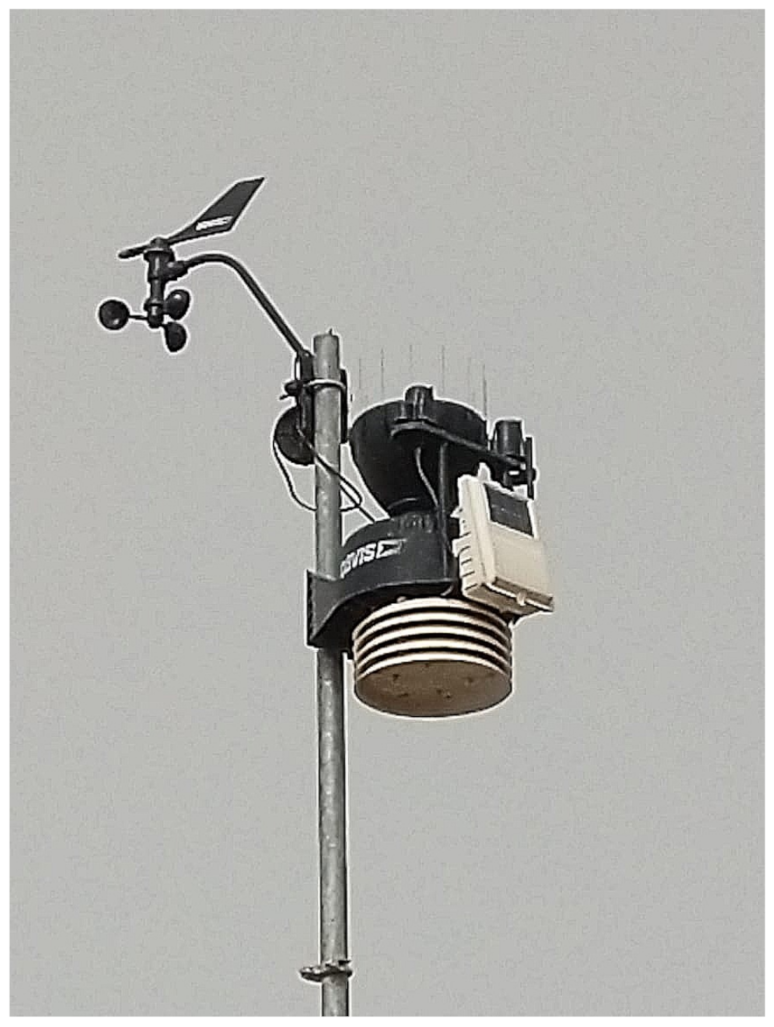
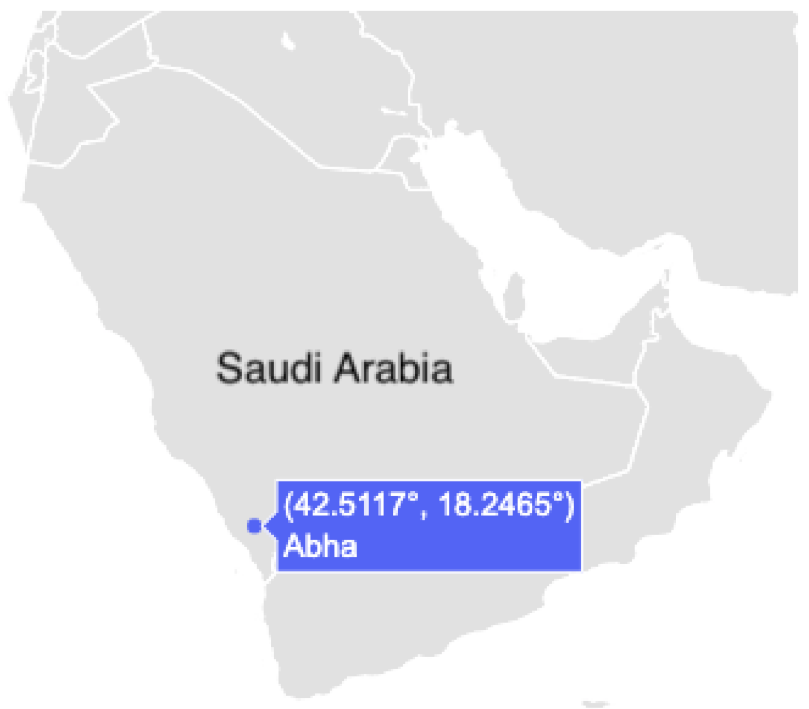
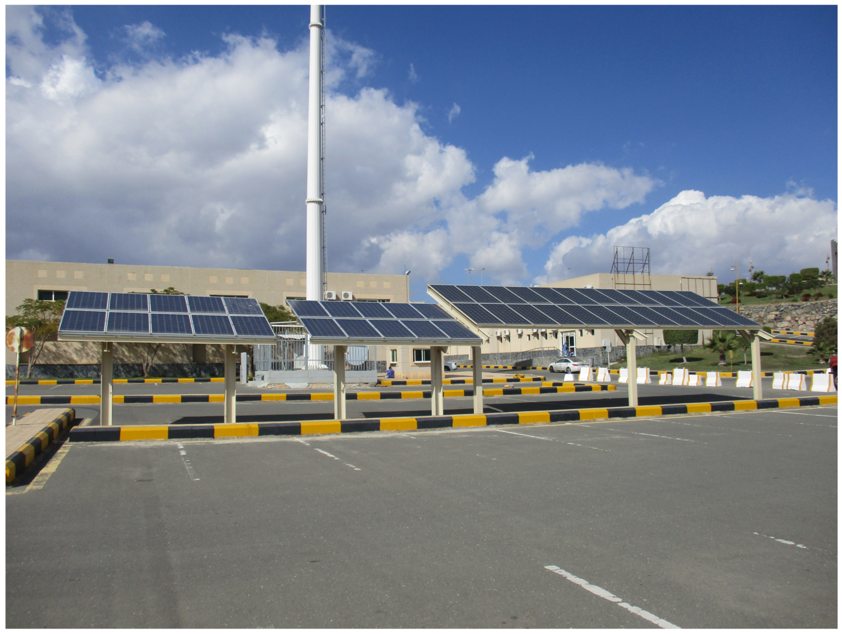
3.1. Site and Instruments

This study was conducted at KKU, located in Abha, Asir, Saudi Arabia. Saudi Arabia is part of the northern hemisphere, centered in West Asia. The country is divided into 13 administrative regions. Abha is the capital of the Asir region, situated 2200 m above sea level in the southwestern part of Saudi Arabia. Its coordinates are 18°13′14.40′′ N and 42°30′15.59′′ E. The solar PV system was installed on a south-facing rooftop at a tilt angle of 22° with the parking lots of the KKU campus, as shown in Figure 1 and Figure 2. For research purposes, it was installed in November 2018 in the College of Engineering, far away from the harsh weather conditions of the marine environment. The selected parameters for the tilt and azimuth angle for the system are shown in

Table 1. Orientation Parameters Selected In the PV System.

Tilt angle	22°
Azimuth angle	−21°
Field type	Fixed tilted plane

. The parameters were selected in accordance with the actual values of the existing system.

As presented in

Table 2. PV Array Parameters and Characteristics.

Mechanical Characteristics
Model	KS-240PC
Solar cells	Polycrystalline silicon 156 × 156 mm
No. of cells	60 (6 × 10)
Dimensions	1663 mm × 998 mm × 35 mm
Weight	23.5 kg
Front glass	4.0 mm tempered glass
Frame	Anodized aluminum alloy
Cell area	2.9 m2
PV module Electrical Characteristics (STC) STC: Standard test condition; 1000 W/m2, 25 °C, AM 1.5
Optimum operating voltage (Vmp) (V)	30.12
Optimum operating current (Imp) (A)	8.21
Open circuit voltage (Voc) (V)	37.94
Short circuit current (Isc) A)	8.69
Maximum power @ STC (Pmax) (W)	240 W
Module efficiency	14.8%
Operating module temperature	−40 °C to +85 °C
Maximum system voltage	1000 V DC (IEC)/600 V DC (UL)
Maximum series fuse rating	20 A
Power tolerance	0/+5%
Temperature Characteristics NOCT: Nominal operating cell temperature, Irradiance level 800 W/m2, Spectrum AM 1.5, Wind velocity 1 m/s, Ambient temperature 20 °C
Nominal operating cell temperature (NOCT)	45 °C ± 2 °C
Temperature coefficient of Pmax	−0.44%/°C
Temperature coefficient of Voc	−0.33%/°C
Temperature coefficient of Isc	−0.055%/°C

, the solar PV system comprises 20 modules of type KS-240PC with one TRIO-5.8-TL-OUTD-400 inverter of 5.8 kW rating. The 20 modules are distributed in a total area of 33.2 m² over one string of the maximum power point tracker (MPPT) for maximum installation flexibility for optimal energy production. This inverter includes two MPPTs and integrates power control, monitoring functionalities, and environmental sensor inputs without the need for any external components. The total installed PV power is 4.80 kWp. The PV array parameters considered here have the following manufacturer parameters. The inverter’s nominal ac power is 5.22 kW and the maximum ac power is 5.8 kVA, as the name indicates. The maximum efficiency is 98% at a voltage level of 175 V. The maximum efficiency is set as 97.5% according to the European efficiency, the average operating efficiency over a yearly power distribution corresponding to the middle-Europe climate. The inverter has two MPPT inputs, which make it possible to connect strings with different panels to one inverter. The nominal power of the two strings connected to the inverter is 4.6 kW ac, which fits well with the inverter’s nominal power.

Radiation measurements were performed by a Pyranometer (Py), as shown in Figure 3). This is a solar irradiance sensor designed to measure the global solar irradiances, which is the amount of solar energy per unit area per unit time incident on a specific orientation surface emanating from a hemispherical field of view.The global solar irradiance includes both direct and diffuse sunlight, and, in some cases, specular reflections of sunlight. Nothwithstanding this, the weather station mentioned in Section 3.2 includes a built-in Py. We observed the SR20-T2 Py to be more precise than the weather station built-in Py, where we validated our reading via the PVsyst software [35]. The Py’s specifications are summarized in

Table 3. SR20-T2 Py Specifications.

Spectral range (20% points)	285 to 3000 10${}^{-9}$ m
Calibration uncertainty	<1.2% (k = 2)
Rated operating temperature range	−40 to +80 °C
Sensitivity	7 to 25 10${}^{-6}$ V/(W/m2)
Impedance	20 to 200
Maximum operational irradiance	2000 W/m2
Response time (95%)	4.5 s
Temperature response	<±1% (−10 to +40 °C) and <±0.4% (−30 to +50 °C) with correction in data processing

.

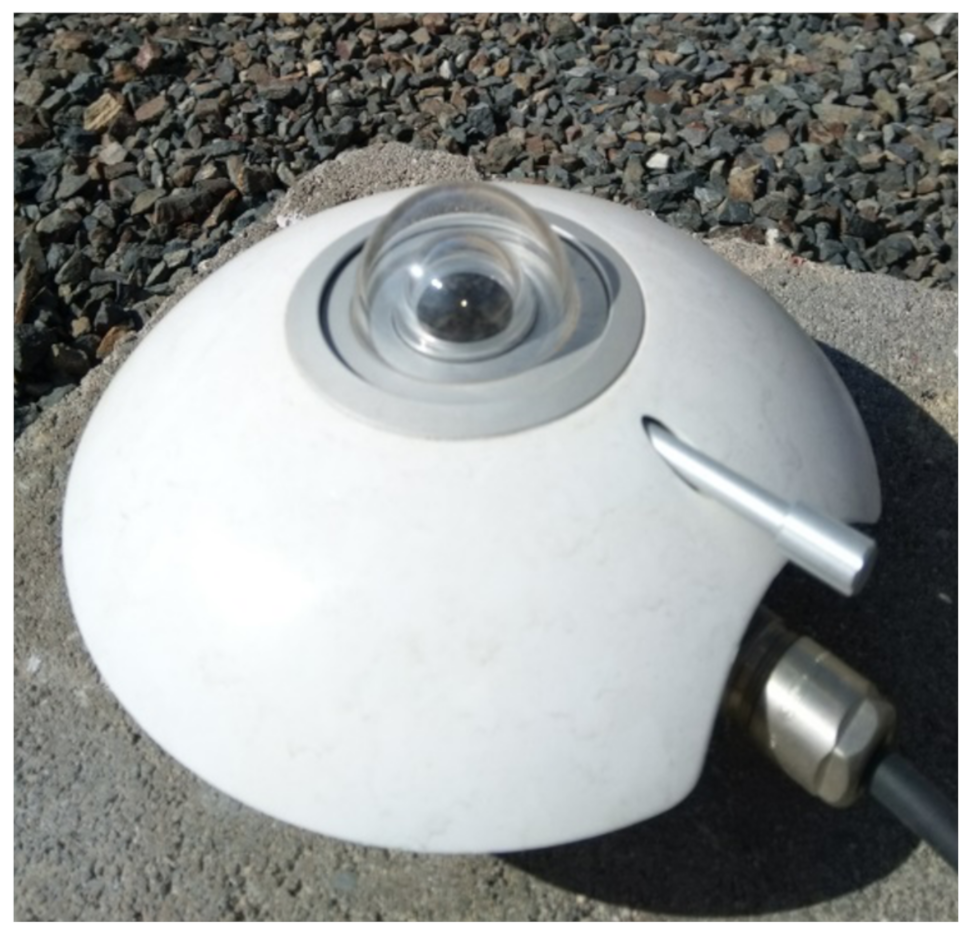
3.2. Weather Station

Figure 4 shows the weather station used in this study, Davis Vantage Pro2, made in the USA. It continuously collects and transmits weather data. It is equipped with several sensors for different parameters such as temperature, pressure, rainfall, solar radiation. The weather station was assembled with the console and the sensor suit. This console and the sensor unit are dual-powered, and have an inbuilt battery and AC-power supply connected as a backup. The sensor suite is succinctly described in

Table 4. The Sensor Suite Consistency.

SI No.	Parameter	Type of Sensor Used
1	Temperature sensor	PN junction silicon diode
2	Wind speed sensor	Solid state magnetic sensor
3	Wind direction sensor	Wind vane with potentiometer
4	Rain collector	Tipping spoon type of Tipping bucket, 0.01′′ per tip (0.2 mm with metric rain adapter)
5	Relative humidity sensor	Film capacitor element
6	Housing material	UV-resistance, ABS, Polypropylene

, and the console equipment that displays the pertinent data is presented in

Table 5. Console Output.

Sl No.	Parameter	Resolution	Range	Accuracy
1	Barometric pressure	0.01′′ Hg, 0.1 mm Hg, 0.1 hPa/mb	16.00′′ to 32.50′′ Hg, 410 to 820 mm Hg, 540 to 1100 hPa/mb	±0.03′′ Hg (±0.8 mm Hg, ±1.0 hPa/mb) (at room temperature)
2	Clock	1 min	12 or 24 h format	±8 s/month
3	Dew point	1 °F or 1 °C. °C is converted from °F rounded to the nearest 1 °C	−105° to +130 °F (−76° to +54 °C)	±3 °F (±1.5 °C) (typical)
4	Evapotranspiration	0.01′′ or 0.1 mm	Daily to 32.67′′ (832.1 mm); Monthly Yearly to 199.99′′ (1999.9 mm)	Greater of 0.01′′ (0.25 mm) or ±5%
5	Forecast	Barometric Reading Trend, Wind Speed Direction, Rainfall, Temperature, Humidity, Latitude Longitude, Time of Year	—–	——–
6	Heat Index	1 °F or 1 °C. °C is converted from °F rounded to the nearest 1 °C	−40° to +165 °F (−40° to +74 °C)	±3 °F (±1.5 °C) (typical)
7	Humidity	1%	1 to 100% RH	±3% (0 to 90% RH), ±4% (90 to 100% RH)
8	Moon phase	1/8 (12.5%) of a lunar cycle, 1/4 (25%) of lighted face on console	New moon, Waxing crescent, First quarter, Waxing gibbous, Full moon, Waning gibbous, Last quarter, Waning crescent	±38 min
9	Rainfall	0.01′′ or 0.2 mm (1 mm at totals ≥2000 mm)	0 to 199.99′′ (0 to 6553 mm)	For rain rates up to 2/h (50 mm/h): ±4% of total or +0.01′′ (0.2 mm) (0.01′′ = one tip of the bucket), whichever is greater. For rain rates from 2/h (50 mm/h) to 4/h (100 mm/h): ±4% of total or +0.01′′ (0.25 mm) (0.01′′ = one tip of the bucket), whichever is greater
10	Rain rate	0.01′′ or 0.1 mm	0, 0.04/h (1 mm/h) to 96/h (0 to 2438 mm/h)	±5% for rates less than 5′′ per hour (127 mm/h)
11	Solar radiation	1 W/m2	0 to 1800 W/m2	±5% of full scale
12	Sunrise and sunset	1 min	Depends	±1 min
13	Temperature	0.1 °F or 1 °F or 0.1 °C or 1 °C (user-selectable) °C is converted from °F rounded to the nearest 1 °C	+32° to +140°F (0° to +60 °C)	±1 °F (±0.5 °C)
14	Temperature humidity Sun wind index	0.1 °F or 1 °F or 0.1 °C or 1 °C (user-selectable) °C is converted from °F rounded to the nearest 1 °C	−90° to +165 °F (−68° to +74 °C)	±4 °F (±2 °C) (typical)
15	Ultra violet (UV) radiation dose	0.1 MEDs to 19.9 MEDs; 1 MED above 19.9 MEDS	0 to 199 MEDs	±5% of daily total
16	UV radiation index	0.1 Index	0 to 16 Index	±5% of full scale
17	Wind direction	16 points (22.5°) on compass rose, 1° in numeric display	0°–360°	±3°
18	Wind speed	1 mph, 1 km/h, 0.4 m/s, or 1 knot (user-selectable). Measured in mph, other units are converted from mph and rounded to the nearest 1 km/h, 0.1 m/s, or 1 knot.	1 to 200 mph, 1 to 173 knots, 0.5 to 89 m/s, 1 to 322 km/h	±2 mph (2 kts, 3 km/h, 1 m/s) or ±5%, whichever is greater

. The maximum capacity of the anemometer is 322 kph (wind speed). This makes the weather station more durable and sensitive to the lightest breeze. The weather station was installed on the rooftop of KKU.

4. Methodology

The methodology that was adopted to build an ideal ML model for Abha’s PV power prediction involved four general phases: (1) data collection and presentation, (2) data preparation (to obtain the data in a suitable format for analysis, exploration, and understanding the data to identify and extract the features required for the model), (3) feature selection and model building (to select the appropriate algorithm and prepare a training and testing dataset), (4) and model evaluation (to observe the final score of the model for the unseen dataset).

4.1. Data Collection and Presentation

As illustrated in the first part of Figure 5, the power generation data extracted from the polycrystalline PV systems placed at KKU are associated with four primary data sources measured over the same period of time. Weather station sensors (WS) were located near the station to measure various parameters, namely ambient temperature (Ta), relative humidity (RH), wind speed (W), wind direction (WD), solar irradiation (SR), and precipitation (R), where solar irradiance was found to be more accurate using the Py sensor. The computed parameters from the WS and Py were also considered. The latter included the solar PV system inverters (N) and panel sensors (PVSR). The four sources of data were utilized together to conduct our experiment. However, the collected data were for December 2019 until February 2020, between the autumn and the winter seasons. During this time, data were acquired and tabulated from sunrise to sunset at an interval of each five minutes for the parameters of low and high temperatures, average temperature, humidity, wind speed, and solar radiations. This differentiated cloudy days, clear-sky days, and mix days. Eventually, about 5000 samples were collected, with different data types such as integer, float, and object. The generated power statistical summary is presented in

Table 6. Statistical Summary for The Generated Power (W).

	Generated Power	Scaled Generated Power
Count	5402	5402
Mean	2336.47108	0
Standard deviation	1569.29464	1
Minimum	0	−1.489
25%	796.435	−0.98145
50%	2460.935	0.07932
75%	3873.59	0.97959
Maximum	5828.5	2.22543

.

Eventually, the collected dataset represented the sensors readings, assuming $\mathbf{A}=\{{\mathbf{a}}_{\mathbf{1}},{\mathbf{a}}_{\mathbf{2}},{\mathbf{a}}_{\mathbf{3}},\dots ,{\mathbf{a}}_{\mathbf{m}}\}$ to be the dataset $\mathit{n}-by-\mathit{m}$ matrix, where $\mathit{n}=$ 5402 is the number of the observations collected from each sensor and the vector ${\mathbf{a}}_{\mathbf{i}}$ is the ith observation with $\mathit{m}=$ 42 attributes, and the generated power p is the target of these features.

4.2. Data Preparation

In general, data need to be pre-processed so that they have a proper format, and are free of irregularities such as missing values, outliers, and inaccurate data values. Missing values are typical in any dataset. They may have occurred during data collection or possibly due to sensor-connecting issues. However, they must be considered by dropping their rows, estimating their values or replacing them. In our case, the data had less than 1% missing values in the total dataset; thus, eliminating these missing values was imperative. Outliers and noisy data emerge due to data entering/transmission errors. We discovered one outlier for “PV Energy”, which we handled by smoothing its value.

Data scaling is typically required because many ML algorithms perform more accurately and converge faster when attributes are on a moderately similar scale and close to normally distributed. In this work, standardization (see Equation (1)) was applied to rescale data to have a mean $\mu (\mathbf{A},\mathbf{p})$ of zero and a standard deviation $\sigma (\mathbf{A},\mathbf{p})$ of one, where the scaled $\mathbf{p}$ is shown in Table 6.

$${(\mathit{a},\mathit{p})}_{\mathit{scaled}}=\frac{({(a,p)}_i-{\mu }_{(}\mathbf{A},\mathbf{p}))}{{\sigma }_{(}\mathbf{A},\mathbf{p})}$$

(1)

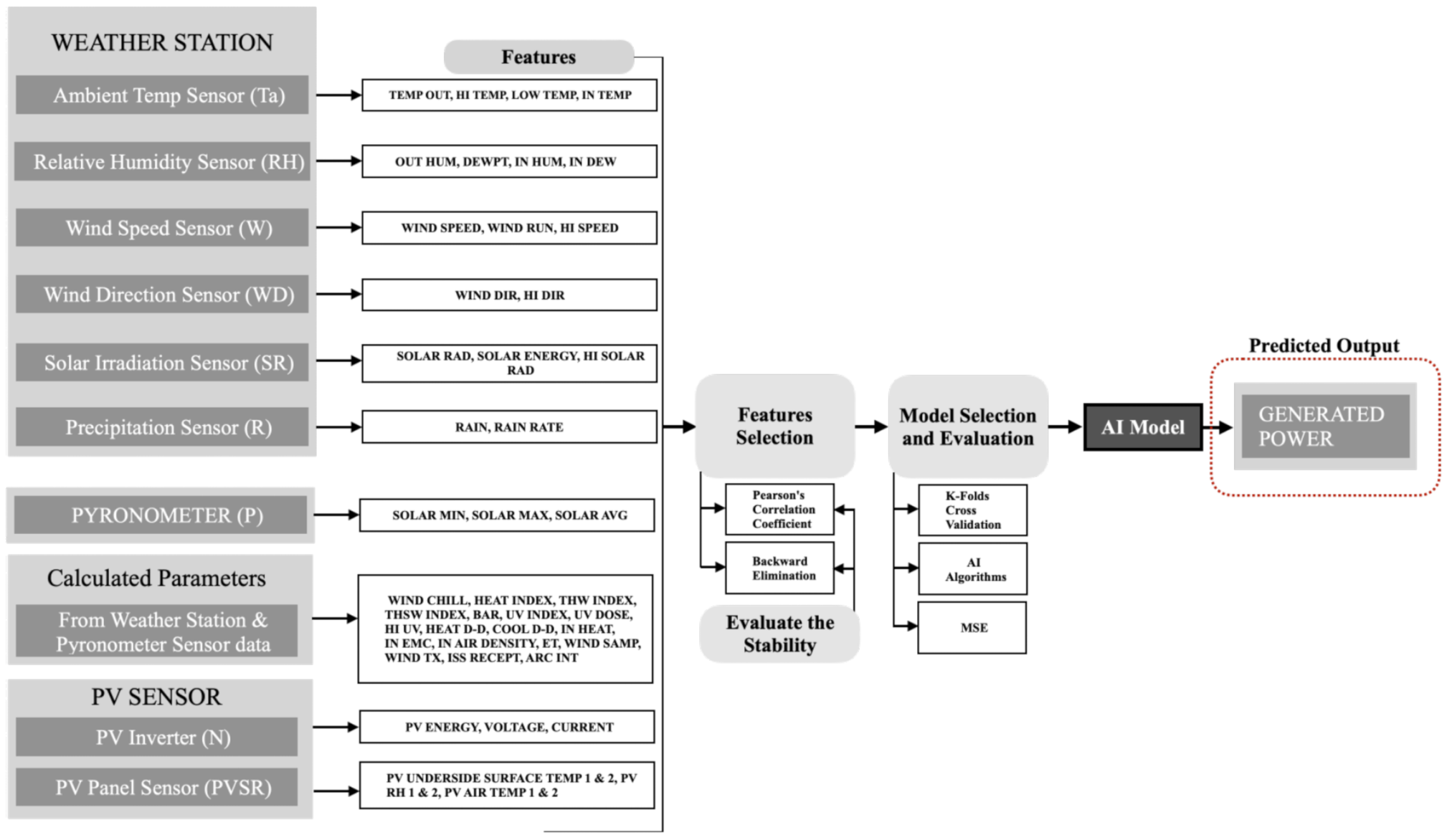
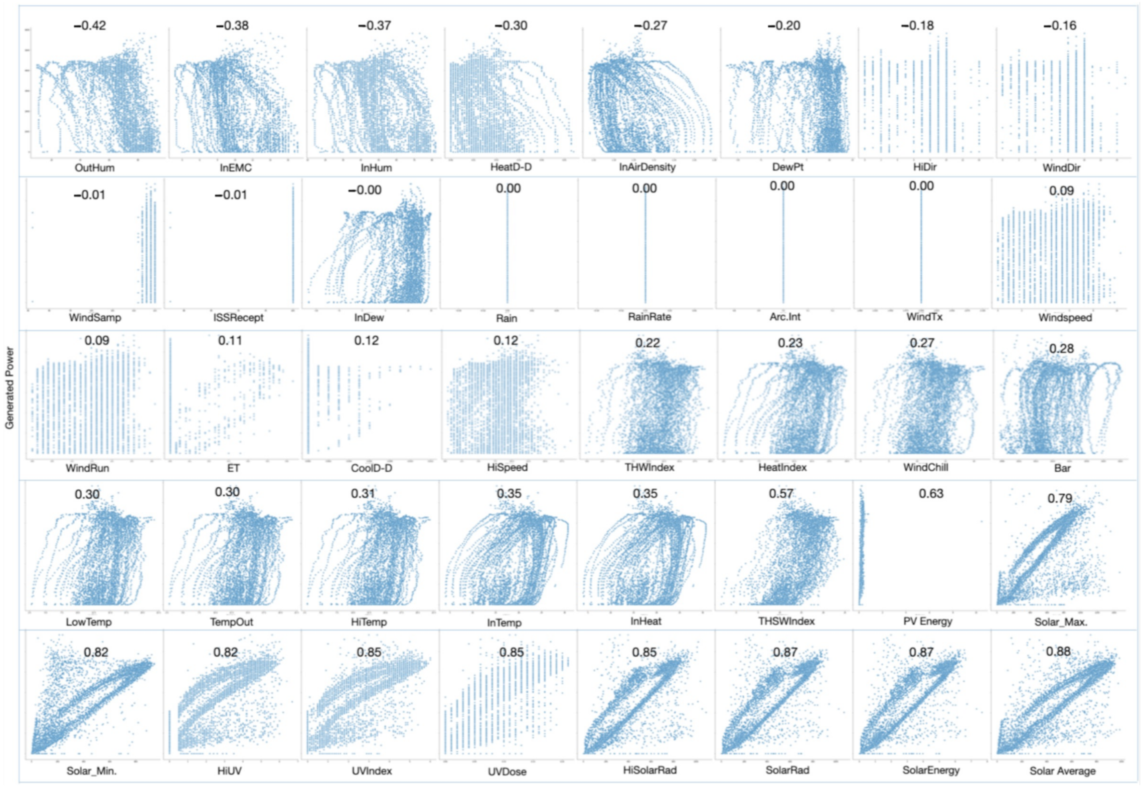
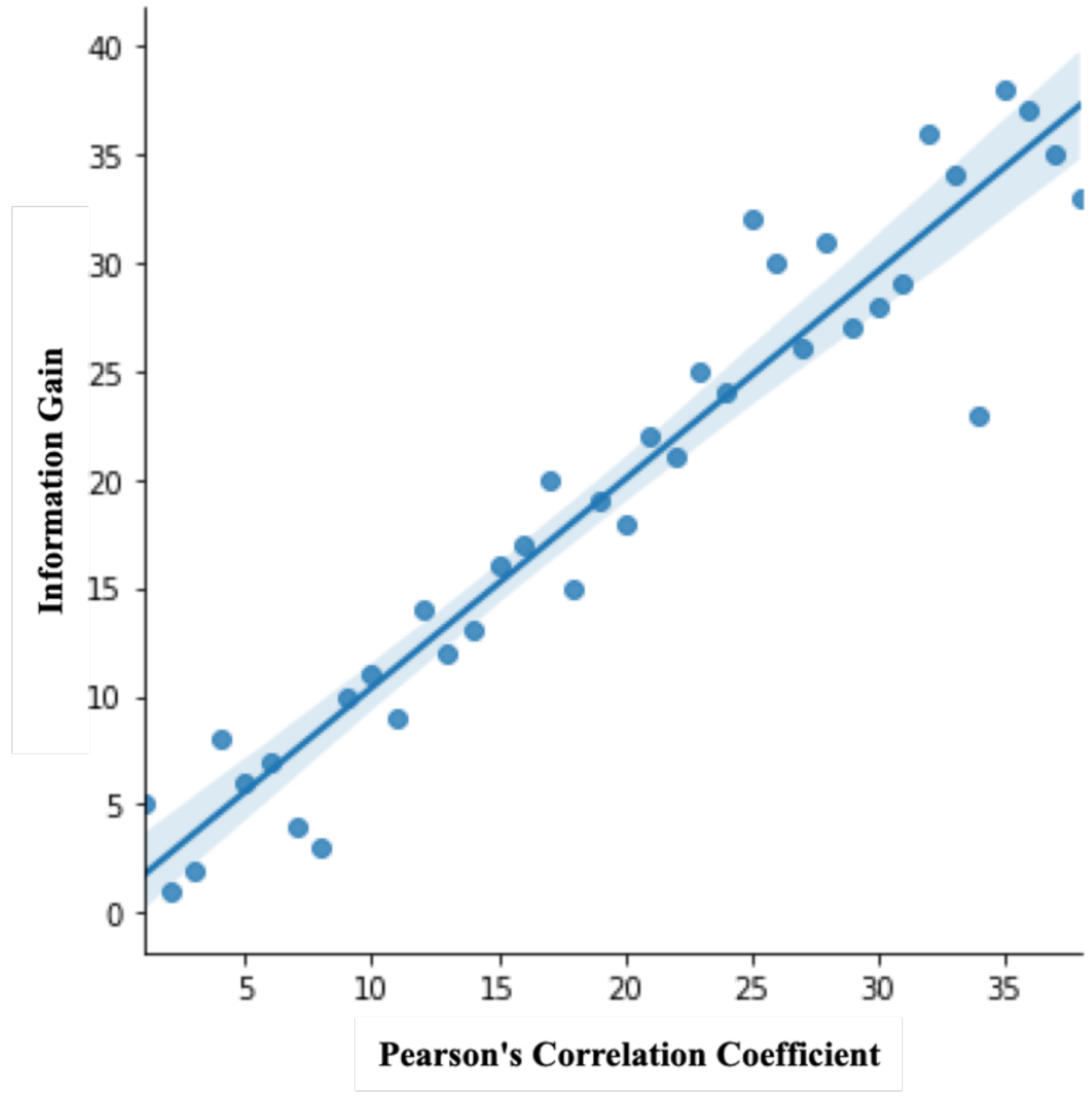
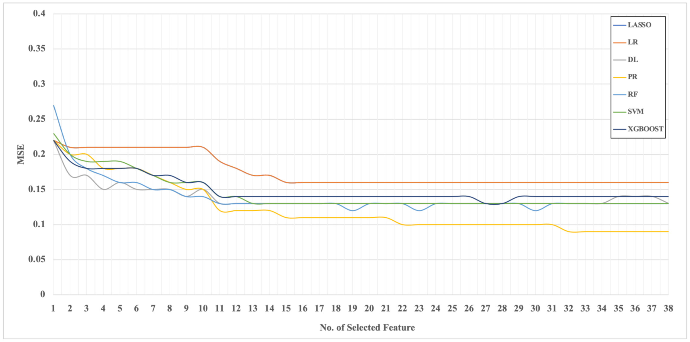
4.3. Feature Selection

Feature selection is one of the core concepts in ML and profoundly affects the model’s performance. Its principal objective is to select the feature set with minimum cardinality while maximizing the learning performance. We believe that, when predicting generated power in the PV system, not every feature equally contributes to the prediction performance. Features can be relevant, partially relevant, or even irrelevant. Feature selection algorithms aim to assign weight to each feature according to its pertinence. As illustrated in Figure 5, in this study, we applied two approaches to score each feature, namely, Pearson’s correlation coefficient [36] (see Equation (2)) and Information Gain [37] (see Equation (3)). The former measures the amount of correlation between each variable and the target, while the latter quantifies the amount of information provided to the class by evaluating the impurity level of each variable using the entropy $H(·)$ with respect to the target.

$$r_{a,p}=\frac{{\sum }_{i=1}^n(a_i-\overline{a})(p_i-\overline{p})}{\sqrt{{\sum }_{i=1}^n{(a_i-\overline{a})}^2}\sqrt{{\sum }_{i=1}^n{(p_i-\overline{p})}^2}}$$

(2)

$$IG(p,a)=H\left(p\right)-\sum _{v\in Values\left(A\right)}\frac{|p_v|}{\left|p\right|}H\left(p_v\right)$$

(3)

The relevant attributes should be sasigned a greater scoring than less relevant attributes. In Equation (2), features were selected by correlating all input sensor parameters with PV-generated power $\mathbf{p}$. Pearson’s Correlation Coefficient Equation (2) was used to evaluate the correlation between the sensor parameters and PV-generated power, where $\mathit{n}$ is the observation size, ${\mathit{a}}_{\mathit{i}}$ and ${\mathit{p}}_{\mathit{i}}$ are the single observation points indexed with $\mathit{i}$, and $\overline{a}$ is the observation mean. A positive and negative correlation score would suggest higher prediction accuracy because an increase in one value of the attribute increases/decreases the generated power value. Meanwhile, zero correlation coefficient indicates no relation. Nevertheless, Figure 6 indicates the amount of correlation of each attribute with the generated power. The Solar Average has the most crucial positive correlation (+ve) with 88%, although the Out Humidity has the most significant negative correlation (−ve) with about −42%. Meanwhile, the rain rate, rain and arc exhibited zero correlation. Furthermore, profound/redundant features that are directly affected by the generated power have been dropped, such as Voltage, Current, PV Energy, and Solar Energy, where the number of attributes were reduced to $\mathit{m}=$ 38.

To evaluate the similarity between two ranked sets of features r represented by $r_{a,p}$ and $\overline{r}$ represented by $IG(p,a)$), Spearman’s rank correlation coefficient [38] (see Equation (4)) was used to assess the significance of the relationship between them.

$$S_R(r,\overline{r})=1-6\sum _i\frac{{(r_i-\overline{r_i})}^2}{m(m^2-1)}$$

(4)

Spearman’s rank correlation coefficient resulted in a range of [−1,1]. The maximum value was reached when the two ranks were equivalent, while the minimum was reached when they were precisely in reverse order and zero meaned no correlation between r and $\overline{r}$. However, after we measured the stability of the two sets of features, we observed them to be stable with the value 0.96. In Figure 7, we show the comparison of two ranked feature lists, where the x-axis and the y-axis represent the Pearson’s correlation coefficient and information gain for features, respectively. Moreover, the linear line shows the stability between them.

Backward elimination was applied after Pearson’s correlation coefficient was calculated, which selected the most appropriate attributes. We started with a complete set of attributes and then recursively removed one attribute after each iteration. The eliminated attribute is the attribute with the lowest absolute correlation coefficient $|r_{a,p}|$. At each iteration, we evaluated the loss using the remaining set of features. The backward elimination criterion was applied from the lowest correlated attribute to the highest, one until only one attribute remained.

4.4. Model Selection and Evaluation

The selection of appropriate ML algorithms to predict the amount of power generated $\widehat{\mathbf{p}}$ based on the sensors’ readings was challenging, because each ML model performs differently on the same dataset according to the model’s nature. A number of ML models need to be trained and tested to select the optimal or superior one. Nonetheless, prior to the training, the dataset needs to be divided into a training set, to build up a model by extracting the features and train them to fit the model, and a testing set, to validate the built model by predicting the outcome of the unseen data. There are numerous methods of splitting the dataset, such as hold-out and cross-validation. As illustrated in the first part of Figure 5, in this experiment, we used k-fold cross-validation with $k=10$. It is known for its ability to reduce overfitting while improving generalizability power. Moreover, cross-validation is known to have a better bias-variance trade-off. Therefore, the models are expected to perform equally well for the unseen data and the training data.

Many classical and modern regression and prediction models were examined in this study to estimate the generated power from the PV system. These include LASSO, RF, LR, PR, XGBoost, SVM, and DL.

The LR model [39] (see Equation (5)) is one of the simplest ML models used to find a linear relationship between the generated power $\mathbf{p}$ and the input parameters $\mathbf{A}$. Taking $\mathbf{y}$ as the response value that lies in the best-fit regression plane, the intercept b in Equation (6) is the reference position of the plane, and ${\mathbf{x}}_{\mathbf{m}}$ is the m predictor variable from the most effective attributes. $w_1,\dots ,w_m$ in Equation (7) are the parameters of slope coefficients. The response variable is the generated power $\mathbf{p}$, and the predictor variables are selected from the most effective attributes $\mathbf{A}$ variables. Nevertheless, Equation (5) can present all the datapoints as a matrix (see (8)). Next, PR [40] (see Equation (9)) is a well-known algorithm, applied when the data are correlated, but the relationships are non-linear. This is a particular case of LR because we created polynomial attributes to fit the polynomial equation, where the dth power is the PR degree. LASSO [41] is also a type of LR model trained with an L1 regularizer in the loss function $J{\left(w\right)}_{L1}=\frac{1}{n}{\sum }_{i=1}^n(f_w{\left(x\right)}_i-y_i)+\lambda {\sum }_{j=1}^n\left|w_j\right|$, to reduce overfitting, which applies shrinkage. Shrinkage is where data values are shrunk toward a central point, where $\lambda$ denotes the amount of shrinkage. However, it is well-suited for data that show high multi-collinearity levels and fewer parameters.

$$y\leftarrow f_w\left(x\right)=b_n+w_1{x}_1+\dots +w_m{x}_m$$

(5)

$$\begin{array}{c}\hfill b_n=\frac{\left({\sum }_{i=1}^n{y}_i\right)\left({\sum }_{i=1}^n{x}_i^2\right)-\left({\sum }_{i=1}^n{x}_i\right)\left({\sum }_{i=1}^n{x}_i{y}_i\right)}{n\left({\sum }_{i=1}^n{x}_i^2\right)-{\left({\sum }_{i=1}^n{x}_i\right)}^2}\end{array}$$

(6)

$$\begin{array}{c}\hfill w_m=\frac{n\left({\sum }_{i=1}^m{x}_i{y}_i\right)\left({\sum }_{i=1}^m{x}_i^2\right)-\left({\sum }_{i=1}^m{x}_i\right)\left({\sum }_{i=1}^m{y}_i\right)}{n\left({\sum }_{i=1}^m{x}_i^2\right)-{\left({\sum }_{i=1}^m{x}_i\right)}^2}\end{array}$$

(7)

$$\begin{array}{c}\hfill \left(\begin{array}{c}{y}_1\\ y_2\\ ⋮\\ y_n\end{array}\right)=\left(\begin{array}{c}{b}_1\\ b_2\\ ⋮\\ b_n\end{array}\right)+\left(\begin{array}{c}{w}_1\\ w_2\\ ⋮\\ w_m\end{array}\right)\left(\begin{array}{cccc}{x}_1& x_2& \cdots & x_m\end{array}\right)\end{array}$$

(8)

$$y=b+w_1{x}_1+w_2{x}_1^2+\dots +w_d{x}_1^d$$

(9)

An RF [42] is an ensemble of randomized regression trees that combine predictions from multiple ML algorithms to make more accurate predictions and control overfitting. XGBoost [43] has evolved as one of the most famous ML algorithms in recent years. It relates to a family of boosting algorithms named the gradient boosting decision tree (GBDT), a sequential technique that operates on the principle of an ensemble as it combines a set of weak learners and delivers an increased prediction accuracy. The most prominent difference between XGBoost and GBDT is that the former uses advanced regularization, such as L1 (LASSO) and L2 (Ridge), which is faster and has less chance of overfitting. An SVM [44] (see Equation (10)) performs a non-linear mapping of the training data to a higher-dimension space over a kernel function $\varphi$. It is possible to perform an LR where the kernel selection defines a more or less efficient model. The radial basis function (RBF) $e^{-\gamma {∥x-y∥}^2}$, as the kernel function, is used as a mapping function.

$$f_w\left(x\right)=\sum _{i=1}^n{w}_i^T\varphi \left(x^i\right)+b$$

(10)

NNs [45,46] have been extensively applied to solve numerous challenging AI problems. They surpass the traditional ML models by dint of their non-linearity, variable synergies, and customizability. The process of building an NN starts with the perceptron. In simple and straightforward terms, the perceptron receives inputs, multiplies them by some weights, and then carries them into an activation function such as a rectified linear unit (ReLU) to generate an output. NNs are designed by adding these perceptron layers together, in what is known as a multi-layer perceptron model. There are three layers of an NN: input, hidden, and output. The input layer immediately receives the data, whereas the output layer produces the required output. The layers in between are called hidden layers, and are where the intermediate computation takes place.

Model evaluation is a critical ML task. It helps to quantify and validate the model’s performance, makes it easy to present the model to others, and ultimately selects the most suitable model. There are various evaluation metrics; however, only a few of these are applicable to regression. In this work, the most common metric used for regression tasks (MSE) is applied to compare the models’ results. MSE (see Equation (11)) is the average of the squared difference between the predicted power $\widehat{\mathbf{p}}$ and the actual power $\mathbf{p}$. This penalizes large errors and is more convenient for optimization, as it is differentiable and has a convex shape.

$$MSE=\frac{1}{n}\sum _{i=1}^n{(\widehat{p_i}-p_i)}^2$$

(11)

Figure 5 schematically presents the overall AI system and methodology used in the research and delineates all the steps from data collection until the computation of predicted power.

5. Results and Discussion

As noted previously and depicted in Figure 7, the two feature-scoring approaches generated very similar results. Therefore, the learning performance was almost equivalent using both approaches. We omitted the results of the information gain to reduce duplication.

The results of the prediction error, illustrated in Figure 8, reveal that all prediction models behave in a similar manner. The DL-based model gave the minimum error with the minimum set of features (approximately seven features). The DL error was steady, with almost over all feature sets’ cardinalities ranging from almost two features up to the full cardinality. Thus, it can be concluded that, when using only a few features or looking for a very stable prediction regardless of the features, DL is preferable.

In contrast, PR’s prediction was the best when the feature set was greater than 10 features. This illustrates the advantageous properties of PR in the extraction of marginally useful knowledge, even from extremely irrelevant features. MSE kept steadily reducing after adding more features. With regard to MSE, PR is the most optimal choice in this case, as it had the lowest value.

As expected, LR had the highest error associated, with erros found over various selected cardinalities. LR is not capable of modeling non-linear relationships. The generated power is nonlinear in this problem. Thus, LR is not a suitable and adequate fit for the model.

LASSO, XGBOOST, SVM, and RF behaved in a similar manner. RF was the worst in terms of MSE in the cases with a single feature. This is intuitive, due to the nature of the algorithm. To build more decision trees, RF requires more features. Thus, one feature was not sufficient to extract sufficient and relevant knowledge in this case. However, SVM was extremely steady after selecting 13 features. This is due to the fundamental nature of SVM, which works by selecting a set of support vectors to maximize the margin. These support vectors are the same beyond the thirteenth feature. This is another way of indicating the proper number of selected features.

Figure 9 illustrates the actual active power versus the predicted one from December 2019 to February 2020 using a PR model. Thus, we can observe that the model can reasonably predict the generated power. However, there are still obstacles to some predictions, due to sudden voltage dips in the original dataset. The latter occured because we applied a transient three-phase voltage dip to gauge the performance of the system under study. The active power output from the whole PV system before the fault was 4000 W. After the occurrence of a fault, a transient peak of 5800 W was instantly observed for the active power generation. Within a short interval, and according to the Saudi grid code [47], the transient was cleared. The solar PV system controller action was sustained to cope with the fault, after which the power oscillations were damped out and the system restored to its regular operation. Therefore, immediately after the fault was cleared, the solar PV system entered a voltage regulation mode [48,49], and the active power generated at the solar PV terminals started to reach the rated values. $\mathbf{p}$ output’s mirrored characteristics are a sign of the controlled converter action, which is only limited by the converter’s nominal current rating.

6. Conclusions and Future Work

In this paper, seven well-known machine learning algorithms were successfully applied to solar PV system data from Abha (Saudi Arabia) to predict the generated power. The prediction error of the algorithms was relatively low. This indicates that we can confidently evaluate the feasibility of installing solar PV systems in residential buildings using only a small set of weather station data. Although the algorithms behaved similarly, the Deep Learning technique gave the minimum error with the minimum set of selected features. However, Polynomial Regression produced the best prediction performance when we incorporated more features.

References

1. Newell, R.; Raimi, D.; Aldana, G. Global Energy Outlook 2019: The Next Generation of Energy. Available online: https://www.rff.org/publications/reports/global-energy-outlook-2019/ (accessed on 11 October 2020).
2. Capuano, L. International Energy Outlook 2018 (IEO2018); US Energy Information Administration (EIA): Washington, DC, USA, 2018; Volume 2018, p. 21.
3. Khan, M.M.A.; Asif, M.; Stach, E. Rooftop PV potential in the residential sector of the Kingdom of Saudi Arabia. Buildings 2017, 7, 46. [Google Scholar] [CrossRef]
4. EIA. FREQUENTLY ASKED QUESTIONS (FAQ). 2020. Available online: https://www.eia.gov/tools/faqs/faq.php?id=86&t=1 (accessed on 24 December 2020).
5. U.S. Energy Information Administration. Total Energy Monthly Data. 2020. Available online: https://www.eia.gov/totalenergy/data/monthly/pdf/mer.pdf (accessed on 24 December 2020).
6. Almaraashi, M. Short-term prediction of solar energy in Saudi Arabia using automated-design fuzzy logic systems. PLoS ONE 2017, 12, e0182429. [Google Scholar] [CrossRef] [PubMed] [Green Version]
7. Mazria, E.; Kershner, K. Meeting the 2030 challenge through building codes. Architecture 2008, 2030. Available online: https://sallan.org/pdf-docs/2030Challenge_Codes_WP-1.pdf (accessed on 24 December 2020).
8. REN21, Global Status Report. Renewable Energy Policy Network for the 21st Century. 2020. Available online: https://www.ren21.net/wp-content/uploads/2019/05/gsr_2020_full_report_en.pdf (accessed on 24 December 2020).
9. SEIA. U.S. Solar Market Insight. 2020. Available online: https://www.seia.org/us-solar-market-insight#:~:text=The%20U.S.%20installed%203.8%20gigawatts,power%2016.4%20million%20American%20homes (accessed on 24 December 2020).
10. Cococcioni, M.; D’Andrea, E.; Lazzerini, B. One day-ahead forecasting of energy production in solar photovoltaic installations: An empirical study. Intell. Decis. Technol. 2012, 6, 197–210. [Google Scholar] [CrossRef]
11. IRENA. Energy Profile Saudi Arabia. 2020. Available online: https://www.irena.org/IRENADocuments/Statistical_Profiles/Middle%20East/Saudi%20Arabia_Middle%20East_RE_SP.pdf (accessed on 24 December 2020).
12. Amran, Y.A.; Amran, Y.M.; Alyousef, R.; Alabduljabbar, H. Renewable and sustainable energy production in Saudi Arabia according to Saudi Vision 2030; Current status and future prospects. J. Clean. Prod. 2020, 247, 119602. [Google Scholar] [CrossRef]
13. Care, K. Building the Renewable Energy Sector in Saudi Arabia; International Renewable Energy Agency: Abu Dhabi, United Arab Emirates, 2012; Available online: https://www.irena.org/-/media/Files/IRENA/Agency/Events/2012/Sep/5/5_Ibrahim_Babelli.pdf (accessed on 24 December 2020).
14. Pazheri, F. Solar power potential in Saudi Arabia. Int. J. Eng. Res. Appl. 2014, 4, 171–174. [Google Scholar]
15. Saber, E.M.; Lee, S.E.; Manthapuri, S.; Yi, W.; Deb, C. PV (photovoltaics) performance evaluation and simulation-based energy yield prediction for tropical buildings. Energy 2014, 71, 588–595. [Google Scholar] [CrossRef]
16. Chowdhury, S.; Taylor, G.; Chowdhury, S.; Saha, A.; Song, Y. Modelling, simulation and performance analysis of a PV array in an embedded environment. In Proceedings of the IEEE 2007 42nd International Universities Power Engineering Conference, Brighton, UK, 4–6 September 2007; pp. 781–785. [Google Scholar]
17. Chouder, A.; Silvestre, S.; Sadaoui, N.; Rahmani, L. Modeling and simulation of a grid connected PV system based on the evaluation of main PV module parameters. Simul. Model. Pract. Theory 2012, 20, 46–58. [Google Scholar] [CrossRef]
18. Al-Dahidi, S.; Ayadi, O.; Adeeb, J.; Louzazni, M.; Hemidat, S.; Saidan, M.; Al-Zu’bi, S.; Nelles, M.; Hamdan, M.A.; Brawiesh, A.K.; et al. Assessment of Artificial Neural Networks Learning Algorithms and Training Datasets for Solar Photovoltaic Power Production Prediction. Front. Energy Res. 2019, 7, 130. [Google Scholar] [CrossRef] [Green Version]
19. Pasion, C.; Wagner, T.; Koschnick, C.; Schuldt, S.; Williams, J.; Hallinan, K. Machine Learning Modeling of Horizontal Photovoltaics Using Weather and Location Data. Energies 2020, 13, 2570. [Google Scholar] [CrossRef]
20. Brahimi, T. Using Artificial Intelligence to Predict Wind Speed for Energy Application in Saudi Arabia. Energies 2019, 12, 4669. [Google Scholar] [CrossRef] [Green Version]
21. Alomari, M.H.; Adeeb, J.; Younis, O. Solar photovoltaic power forecasting in jordan using artificial neural networks. Int. J. Electr. Comput. Eng. (IJECE) 2018, 8, 497. [Google Scholar] [CrossRef]
22. Mawson, V.J.; Hughes, B.R. Deep learning techniques for energy forecasting and condition monitoring in the manufacturing sector. Energy Build. 2020, 217, 109966. [Google Scholar] [CrossRef]
23. Kharlova, E.; May, D.; Musilek, P. Forecasting Photovoltaic Power Production using a Deep Learning Sequence to Sequence Model with Attention. In Proceedings of the IEEE 2020 International Joint Conference on Neural Networks (IJCNN), Glasgow, UK, 19–24 July 2020; pp. 1–7. [Google Scholar]
24. Antonanzas, J.; Osorio, N.; Escobar, R.; Urraca, R.; Martinez-de Pison, F.J.; Antonanzas-Torres, F. Review of photovoltaic power forecasting. Sol. Energy 2016, 136, 78–111. [Google Scholar] [CrossRef]
25. Pierro, M.; Bucci, F.; De Felice, M.; Maggioni, E.; Moser, D.; Perotto, A.; Spada, F.; Cornaro, C. Multi-Model Ensemble for day ahead prediction of photovoltaic power generation. Sol. Energy 2016, 134, 132–146. [Google Scholar] [CrossRef]
26. Rajabalizadeh, S.; Tafreshi, S.M.M. A Practicable Copula-Based Approach for Power Forecasting of Small-Scale Photovoltaic Systems. IEEE Syst. J. 2020, 14, 4911–4918. [Google Scholar] [CrossRef]
27. Wee, Y.N.; Nor, A.F.M. Prediction of Rooftop Photovoltaic Power Generation Using Artificial Neural Network. In Proceedings of the 2020 IEEE Student Conference on Research and Development (SCOReD), Johor, Malaysia, 27–29 September 2020; pp. 346–351. [Google Scholar]
28. Sabzehgar, R.; Amirhosseini, D.Z.; Rasouli, M. Solar power forecast for a residential smart microgrid based on numerical weather predictions using artificial intelligence methods. J. Build. Eng. 2020, 32, 101629. [Google Scholar] [CrossRef]
29. Monteiro, C.; Fernandez-Jimenez, L.A.; Ramirez-Rosado, I.J.; Muñoz-Jimenez, A.; Lara-Santillan, P.M. Short-term forecasting models for photovoltaic plants: Analytical versus soft-computing techniques. Math. Probl. Eng. 2013, 2013, 767284. [Google Scholar] [CrossRef] [Green Version]
30. Wei, C.C. Evaluation of Photovoltaic Power Generation by Using Deep Learning in Solar Panels Installed in Buildings. Energies 2019, 12, 3564. [Google Scholar] [CrossRef] [Green Version]
31. Amarawardhana, K.N.; Jayasinghe, S.D.; Shahnia, F. Grid-interactive rooftop photovoltaic clusters with third-party ownership. Int. J. Smart Grid Clean Energy 2020, 9, 102–111. [Google Scholar] [CrossRef]
32. Tuohy, A.; Zack, J.; Haupt, S.E.; Sharp, J.; Ahlstrom, M.; Dise, S.; Grimit, E.; Mohrlen, C.; Lange, M.; Casado, M.G.; et al. Solar forecasting: Methods, challenges, and performance. IEEE Power Energy Mag. 2015, 13, 50–59. [Google Scholar] [CrossRef]
33. Pelland, S.; Remund, J.; Kleissl, J.; Oozeki, T.; De Brabandere, K. Photovoltaic and solar forecasting: State of the art. IEA PVPS Task 2013, 14, 1–36. [Google Scholar]
34. Awan, A.B.; Zubair, M.; Abokhalil, A.G. Solar energy resource analysis and evaluation of photovoltaic system performance in various regions of Saudi Arabia. Sustainability 2018, 10, 1129. [Google Scholar] [CrossRef] [Green Version]
35. Kandasamy, C.; Prabu, P.; Niruba, K. Solar potential assessment using PVSYST software. In Proceedings of the 2013 IEEE International Conference on Green Computing, Communication and Conservation of Energy (ICGCE), Chennai, India, 12–14 December 2013; pp. 667–672. [Google Scholar]
36. Lee Rodgers, J.; Nicewander, W.A. Thirteen ways to look at the correlation coefficient. Am. Stat. 1988, 42, 59–66. [Google Scholar] [CrossRef]
37. Cover, T.M.; Thomas, J.A. Entropy, relative entropy and mutual information. Elem. Inf. Theory 1991, 2, 12–13. [Google Scholar]
38. Kalousis, A.; Prados, J.; Hilario, M. Stability of feature selection algorithms: A study on high-dimensional spaces. Knowl. Inf. Syst. 2007, 12, 95–116. [Google Scholar] [CrossRef] [Green Version]
39. Chung, C.J.F.; Fabbri, A.G.; Van Westen, C.J. Multivariate regression analysis for landslide hazard zonation. In Geographical Information Systems in Assessing Natural Hazards; Springer: Berlin/Heidelberg, Germany, 1995; pp. 107–133. [Google Scholar]
40. Ostertagová, E. Modelling using polynomial regression. Procedia Eng. 2012, 48, 500–506. [Google Scholar] [CrossRef] [Green Version]
41. Xu, H.; Caramanis, C.; Mannor, S. Robust regression and lasso. IEEE Trans. Inf. Theory 2010, 56, 3561–3574. [Google Scholar] [CrossRef] [Green Version]
42. Liaw, A.; Wiener, M. Classification and regression by randomForest. R News 2002, 2, 18–22. [Google Scholar]
43. Chen, T.; Guestrin, C. XGBoost: A Scalable Tree Boosting System. Available online: https://dl.acm.org/doi/abs/10.1145/2939672.2939785 (accessed on 24 December 2020).
44. Chang, C.C.; Lin, C.J. Training v-support vector regression: Theory and algorithms. Neural Comput. 2002, 14, 1959–1977. [Google Scholar] [CrossRef]
45. Specht, D.F. A general regression neural network. IEEE Trans. Neural Netw. 1991, 2, 568–576. [Google Scholar] [CrossRef] [PubMed] [Green Version]
46. Hopfield, J.J. Artificial neural networks. IEEE CIrcuits Devices Mag. 1988, 4, 3–10. [Google Scholar] [CrossRef]
47. Sa, N.G. The Saudi Arabian Grid Code, Electronic Update as of February 2020. 2020. Available online: https://www.ecra.gov.sa/ar-sa/ECRARegulations/Codes/Documents/SAGC%20Electronic%20Update.pdf (accessed on 24 December 2020).
48. Saidi, A.S. Impact of large photovoltaic power penetration on the voltage regulation and dynamic performance of the Tunisian power system. Energy Explor. Exploit. 2020, 38, 1774–1809. [Google Scholar] [CrossRef]
49. Saidi, A.S. Investigation of Structural Voltage Stability in Tunisian Distribution Networks Integrating Large-Scale Solar Photovoltaic Power Plant. Int. J. Bifurc. Chaos 2020, 30, 2050259. [Google Scholar] [CrossRef]
Figure 1. Geographical Location of Abha.
Energies 14 06759 g001
Figure 2. The Installed solar PV system at KKU.
Energies 14 06759 g002
Figure 3. SR20-T2 Py.
Energies 14 06759 g003
Figure 4. Rooftop Weather Station.
Energies 14 06759 g004
Figure 5. Block Diagram of the System.
Energies 14 06759 g005
Figure 6. Correlation Plots.
Energies 14 06759 g006
Figure 7. Spearman’s Rank Correlation Coefficient.
Energies 14 06759 g007
Figure 8. Results attained with various ML techniques.
Energies 14 06759 g008
Figure 9. Results.
Energies 14 06759 g009