Case Study of Multi-Period MILP HENS with Heat Pump and Storage Options for the Application in Energy Intensive Industries

Abstract

The environmental goals of initiatives such as the European Green Deal, which aims to achieve climate neutrality for the EU by 2050, increase the importance of improving and optimizing industrial processes. Mathematical optimization methods like heat exchange network synthesis (HENS) are crucial tools in enabling industry to identify potential energy savings and cost reductions. The lack of publicly available industry data suitable for comprehensive testing of novel optimization procedures is often a major obstacle in development and research. To tackle this problem for extended HENS with potential heat pump and storage integration and show the potential of energy integration in energy-intensive industries (EII), the authors introduce a set of four use-cases based on representative industrial processes from the EII. The application of a previously presented a HENS approach for the integration of heat pumps and storage on these cases resulted in a potential reduction of total annual costs up to 55.43% and total external energy demand up to 87.1%. The presented cases, their solutions, and the open-access mathematical formulation of the optimization procedure make a valuable contribution to the literature and future research in the field of HENS.

1. Introduction

With a share of around 25% of the final energy consumption in the European Union, the industrial sector plays an essential role in the ongoing transition necessary to reach the target of carbon neutrality [1]. A certain part of the industry, the energy-intensive industries (EII), which mainly consist of the sectors iron and steel, refineries, cement, petrochemicals, fertilizer, lime and plaster, pulp and paper, aluminum, inorganic chemicals, and hollow glass, account for 85% of Europe’s industrial greenhouse gas (GHG) emissions. Especially for these EII, the planned climate neutrality by mid-century is coupled with drastic changes in production. The most promising adaption options are reducing energy demand through efficiency improvement, using clean energy sources in the form of renewable electricity or carbon-neutral energy carriers, and utilizing carbon capture and storage technologies. Major obstacles for these measures are that over short time horizons, traditional investments like capacity expansion often offer a better return, and the lower costs of comparable fossil technologies [2]. To lower these barriers as much as possible, the optimal integration of emission-reducing technologies, and thus research in mathematical optimization of processes, plays a crucial role in the energy transition. Independent of the type of optimization, extensive tests with example data sets are needed to evaluate and verify the capabilities of novel approaches. Often industrial data in the right quality or amount are not available, or existing data from the literature are insufficient or unsuitable. This problem was also encountered during previous work on the development of an approach for multi-period mixed integer linear programming (MILP) heat exchange network synthesis (HENS) with simultaneous integration of storage (ST) and heat pumps (HP) presented in [3].

In this approach, the introduction of HP and ST to HENS represents the before mentioned measures of improving energy efficiency by the possibility of shifting thermal energy over time and usage of renewable electricity through HP. Since suitable multi-period example data for proof of concept was not available in the literature, a previously used test case was extended to multiple time periods to show how the approach is able to properly integrate HP and ST into heat exchange networks.

HENS is an extensively researched and prominent topic which shows in the high number of recently published studies. They deal with the different aspects of HENS, for example, with cost-optimal HENS [4], practical retrofitting of HEN [5], or the consideration of different types of heat exchangers (HEX) in HENS [6]. Case studies for different HENS procedures show some difficulties, as explained in the following. For basic single period HENS, the results of different solvers are generally comparable. An example is a case study comparison by Escobar and Trierweiler [7], where some of the most cited example cases, such as the stream data introduced in [8,9] are analyzed. Because these cases only deal with continuous operation in one thermodynamic state and only basic HEN solutions with HEX and utilities are considered, solutions of different optimization approaches are reasonably comparable. In contrast to this, the solutions of multi-period HENS solvers are often not directly comparable, which is due to the different approaches that are used. Further extended multi-period HENS solutions that integrate HP and ST options are even more specific because of the possible placement of installations or the cost coefficients used in the different approaches.

For multi-period HENS, only a tiny number of examples can be found in the literature, like the stream data presented in [10,11]. The cases used or introduced in these studies are given for several time periods, but their operational temperatures lay mostly out of the physical boundaries of HP and are therefore not suitable for usage in this work. Other multi-period stream data are used with wholly different approaches like the heat recovery loop approach by Stampfli et al. [12]. This approach focuses more on selecting the optimum HP technology than the optimized integration of given components by using wholly different optimization targets and specific cost coefficients.

As already stated in [3], mixed-integer programming optimizations solutions are sensitive to changes of parameters in the cost function, on account of its combinatorial nature. This means those cost coefficients that have to be assumed because they are not available for given problems, like for HP or ST cost, strongly impact the specific solutions. Because of this, a meaningful comparison of the resulting networks or the total annual cost (TAC) with solutions of cases dealt with in the literature is nearly impossible. We therefore limit ourselves in this paper to comparing the solutions without ST and HP with the solutions with possible HP and ST installations obtained using the described optimization program.

For a more comprehensive evaluation of the approach presented in [3], to show the potential of HP and ST integration for EII, and to augment the existing literature, it was decided to generate a set of example problems, which are described in Section 2 below. These cases are based on information from the detailed energy analyses of a wide variety of processes provided by Hamel et al. [13], which provide flowcharts and energy balances of 108 prominent industrial processes. In combination with the optimization results obtained with the application of the approach explained in Section 1.2, these example problems are intended to extend the possibility of evaluating future multi-period HENS approaches, with an emphasis on the integration of renewable energy sources and contributing to the existing literature.

1.1. Objectives, Novelty and Contribution

As elaborated above, the development and verification of optimization approaches relies on the availability of suitable data. Contrary to HENS studies like the case study by Escobar et al. [7], the analyses by Floudas et al. [10], or the case study by Zhang et al. [11], where only the integration of HEX between the streams and utility HEX are considered, the possible integration of HP and ST has stricter thermodynamicall requirements for suitability of stream data. Because no cases found, either from industry or the literature, satisfyingly fulfill these requirements, this work aimed to provide suitable cases for further research in the area of HENS with HP and ST integration and to show the potential of energy integration for energy integration in EII. Therefore we consider our main contribution in the introduction of four use-cases for HENS that

• Are based on the thermal requirements of representative real industrial processes from different sectors of the EII;
• Have varying potentials for energy shifting and the integration of renewable energy sources;
• Lay within the operational temperature range of HP.

On the one hand, analysis of the presented cases in described in Section 1.2 shows the potential of HP and ST integration for reducing energy demand and costs for different sectors of the EII. On the other hand, the introduced cases with their corresponding solutions and the fully given and open-access mathematical formulation of the optimization procedure are a valuable base for future research in the area.

1.2. Applied MILP HENS Optimization Tool

As mentioned in the Introduction, the implementation of new example cases presented in this paper results from the need for data to support extended testing of the multi-period MILP HENS with simultaneous integration of ST and HP approach presented in [3].

The setup of the stage-wise superstructure of this approach is shown in Figure 1 with all its possible connections and installations. A set of hot streams (Hs) and cold streams (Cs) that have to reach a defined target temperature represent the demands of a given process. The possible installations for each stage in each timestep are heat exchangers (HEX) between every Hs and every Cs, HEX between the streams and the storages, and HP between a two tank storage and the streams. If more than one installation is chosen for one stream in a stage, the stream is split at the beginning of the stage and mixed isothermally at the end of the stage. Utilities are only permitted after the last and before the first stage. If the same HEX location is selected in more than one timestep, the largest HEX surface area is chosen, and bypasses are assumed for the other timesteps. The cost function given in Equation (A1) of Appendix A consists of step fixed investment costs and variable investment costs for all installations, and energy costs for external energy demand. The optimization finds the best combination of the possible installations to minimize the cost function while assuring that all streams reach their required target temperature. The simplifications necessary for the linearization of the problem formulation come with the introduction of uncertainties in the calculations. This negative aspect is canceled out by the multiple advantages, like the reduction of the mathematical complexity, which reduces the calculation effort and thus processing time. The linearity of the approach eliminates the need for an initial solution, which is often difficult to find for mixed-integer problems. Moreover, the linear and convex optimization procedure always results in a globally optimal solution under the consideration of all given boundaries. These improvements allow for quick and easy analysis of a wide range of problems.

For reasons of completeness, the full mathematical formulation of the applied MILP HENS from Prendl et al. [3] is given in Appendix A in Equations (A1)–(A13).

2. Test Cases

Four processes representative for the EII described in Section 1 have been chosen to analyze the potential improvement by introducing HP and ST with the help of the optimization approach described in Section 1.2. The processes are a weaving mill for human-made fiber (case 1), a pulp mill (case 2), an alkalies and chlorine process (case 3), and a PVC-suspension process (case 4). As explained earlier in Section 1, the data given by the literature are often not suitable for specific approaches without additional assumptions caused by the lack of essential information. The process data from [13], which are used as the base case, are only given for continuous operation in one particular state as energy balances of the different process steps. To generate suitable use-cases, the processes are analyzed to extract streams that have properties suitable for heat exchange between streams. The extracted inlet temperatures and outlet temperatures of this streams are given in the stream data

Table 1. Stream data and cost coefficients for case 1.

			CP	CP	CP	CP
Stream	${\mathit{T}}_{\mathbf{in}}$ (°C)	${\mathit{T}}_{\mathbf{out}}$ (°C)	(kW/K)	(kW/K)	(kW/K)	(kW/K)	h (kW/m${}^2$K)
			Period 1	Period 2	Period 3	Period 4
Hs1	200	100	20	40	10	40	0.5
Hs2	190	90	20	20	20	20	0.5
Hs3	60	30	100	20	100	20	0.5
Hs4	70	30	35	25	35	25	0.5
Hs5	120	80	40	40	40	40	0.5
Cs1	25	150	14	20	14	60	0.5
Cs2	25	70	150	70	150	70	0.5
Cs3	95	130	40	10	140	10	0.5
Hu	200	200	-	-	-	-	1
Cu	10	15	-	-	-	-	1

HEX cost = (4000 + 500${\left[\mathrm{A}\left({\mathrm{m}}^2\right)\right]}^{\beta }$) €${\mathrm{y}}^{-1}$, ST cost 1T = 28,000 €${\mathrm{y}}^{-1}$, ST cost 2T = (7000 + 0.15[$\mathrm{kg}$]) €${\mathrm{y}}^{-1}$, hot utility cost = 0.2 €${\mathrm{kW}}^{-1}{\mathrm{h}}^{-1}$, cold utility cost = 0.02 €${\mathrm{kW}}^{-1}{\mathrm{h}}^{-1}$, $\beta =0.83$, $dTmin=5$ ${}^{\circ }\mathrm{C}$ electrical power costs = 0.03 €${\mathrm{kW}}^{-1}{\mathrm{h}}^{-1}$, HP cost = 11,000 €${\mathrm{y}}^{-1}$ period durations: ${\tau }_1=2$$\mathrm{h}$, ${\tau }_2=3$$\mathrm{h}$, ${\tau }_3=2$$\mathrm{h}$, ${\tau }_4=1$$\mathrm{h}$.

,

Table 2. Stream data for case 2.

			CP	CP	CP	CP
Stream	${\mathit{T}}_{\mathbf{in}}$ (°C)	${\mathit{T}}_{\mathbf{out}}$ (°C)	(kW/K)	(kW/K)	(kW/K)	(kW/K)	h (kW/m${}^2$K)
			Period 1	Period 2	Period 3	Period 4
Hs1	170	20	9	9	12	9	0.5
Hs2	110	60	16	32	40	16	0.5
Hs3	60	40	26	26	70	26	0.5
Cs1	25	170	15	6	8	18	0.5
Cs2	55	100	20	40	20	30	0.5
Cs3	30	80	20	6	10	24	0.5
Hu	200	200	-	-	-	-	1
Cu	10	15	-	-	-	-	1

period durations: ${\tau }_1=1$$\mathrm{h}$, ${\tau }_2=1$$\mathrm{h}$, ${\tau }_3=1$$\mathrm{h}$, ${\tau }_4=1$$\mathrm{h}$.

,

Table 3. Stream data for case 3.

			CP	CP	CP	CP
Stream	${\mathit{T}}_{\mathbf{in}}$ (°C)	${\mathit{T}}_{\mathbf{out}}$ (°C)	(kW/K)	(kW/K)	(kW/K)	(kW/K)	h (kW/m${}^2$K)
			Period 1	Period 2	Period 3	Period 4
Hs1	80	60	50	50	20	50	0.5
Hs2	110	35	110	150	110	160	0.5
Hs3	110	35	60	60	60	60	0.5
Hs4	100	40	40	40	40	40	0.5
Cs1	25	80	120	120	120	120	0.5
Cs2	60	100	130	70	130	60	0.5
Cs3	25	95	40	70	40	60	0.5
Cs4	40	85	30	30	30	30	0.5
Hu	200	200	-	-	-	-	1
Cu	10	15	-	-	-	-	1

period durations: ${\tau }_1=2$$\mathrm{h}$, ${\tau }_2=1$$\mathrm{h}$, ${\tau }_3=2$$\mathrm{h}$, ${\tau }_4=1$$\mathrm{h}$.

and

Table 4. Stream data for case 4.

			CP	CP	CP
Stream	${\mathit{T}}_{\mathbf{in}}$ (°C)	${\mathit{T}}_{\mathbf{out}}$ (°C)	(kW/K)	(kW/K)	(kW/K)	h (kW/m${}^2$K)
			Period 1	Period 2	Period 3
Hs1	80	25	40	60	40	0.5
Hs2	120	90	90	120	40	0.5
Hs3	180	25	50	60	12	0.5
Cs1	26	60	35	20	50	0.5
Cs2	50	80	60	90	70	0.5
Cs3	50	150	40	40	40	0.5
Cs4	90	180	40	24	16	0.5
Cs5	25	120	40	40	30	0.5
Hu	200	200	-	-	-	1
Cu	10	15	-	-	-	1

period durations: ${\tau }_1=1$$\mathrm{h}$, ${\tau }_2=1$$\mathrm{h}$, ${\tau }_3=1$$\mathrm{h}$.

. Because the energy balances in [13] are scaled down to energy demand per produced unit, the heat capacities are scaled to plant sizes suitable for the optimization procedure, while the ratios of the heat capacities of the streams are kept constant for the first operational period p. The stream data are extended for multiple periods, assuming that parts of the processes change over time depending on the product or startup or shutdown processes, to generate suitable example cases for heat pump and storage integration. Cases 1-3 are extended to four, and case 4 to three time periods. The cases are assumed to repeat cyclically over the annual operation time of 8600 h. Care was taken to ensure that timely mismatch of excess energy and energy demand occurs to generate possible opportunities for storages. Often, multi-period test cases in the literature consist of equal time periods for reasons of simplification as in [14], where stream data from [10] are used and adapted to be usable for the applied method. To test the optimization procedure on its ability to deal with a broader range of applications, the duration of the periods is varied for two of the cases.

The same hot utilities (Hu) and cold utilities (Cu) are given for all processes. Furthermore, the possible ST and HP options are the same for all examined cases.

As utilities, steam with an inlet and outlet temperature of 200 ${}^{\circ }\mathrm{C}$ and hot utility costs of $c_{hu}=$ 0.2 €${\mathrm{kWh}}^{-1}$, and cold water with an inlet temperature of 10 ${}^{\circ }\mathrm{C}$ and an outlet temperature of 15 ${}^{\circ }\mathrm{C}$ with cold utility costs of $c_{cu}=$ 0.02 €${\mathrm{kWh}}^{-1}$ are given. As HP option, the linearized HP in [3] is used with the following boundaries: The power consumption of the HP lies in the range from $Pe{l}_{min}=400$ kW to $Pe{l}_{max}=2000$ kW while the possible temperature lift of the HP ranges from $\Delta T_{hpmin}=20$ K to $\Delta T_{hpmax}=50$ K. The maximum condensation temperature of the HP is 115 °C. The lower boundary of the COP is set to $CO{P}_{min}=3$, and the HP approach temperature is chosen as $T_{hpap}=5$ K. The heat transfer coefficient of the HP is assumed with $h_{hp}=5$ kWm${}^{-2}$K${}^{-1}$.

The one tank ST uses thermo-oil as storage medium with a heat capacity of $c{p}_{oil1T}=1.5$ kJkg${}^{-1}$K${}^{-1}$ and a heat transfer coefficient of $h_{oil}=0.5$ kWm${}^{-2}$K${}^{-1}$. The thermo-oil used by the two tank St has the same heat transfer coefficient but a higher heat capacity of $c{p}_{oil2T}=2$ kJkg${}^{-1}$K${}^{-1}$. The one tank storage has a fixed size of 100,000 kg while its operational temperature is optimized during the HENS. The two tank storage has a variable size, but the temperatures of the two tanks, 70 °C and 100 °C, are preset. The remaining cost coefficients used for all cases are given at the bottom of Table 1. In the following subsections, the individual cases are described in detail:

2.1. Case 1

According to the analyses by Shen et al. [15], comparing human-made fiber production around the world, the processes involved have considerable potential for energy optimization. The growing customer demand for environmentally friendly products has increased the industry’s willingness to invest in measures to tap this potential. The streams suitable for HENS within the process include pulp slurry that needs to be heated (Cs1) or cooled (Hs2), process water for mixing (Cs2) or cooling (Hs3), process air (Hs3, Hs4), and flue gases (Hs1). As shown in Table 1, where the stream data for case 1 are given, the streams operate in a range from 25 °C to 200 °C. The overlapping temperature intervals of the Hs and the Cs show potential for heat exchange between the streams. The accumulated heat flows of the individual streams range from 350 kW to 7500 kW. Without the possibility of energy transfer between the time periods and assuming no thermodynamic restrictions exist, the minimum heat surplus or demand can be simplified estimated by adding the heat flows of the Hs and subtracting the heat flows of the Cs for each time period. This minimum is in reality only reachable, if the heating and cooling demands fulfill all thermodynamic requirements for heat transfer and is thus only used for a first estimation. For case 1, this results in a theoretical heat surplus of 100 kw in period 1 and a heat surplus of 3200 kW in period 2, while period 3 and 4 have a heat demand of 4400 kW and 1800 kW, respectively. The timely mismatch of energy surplus and demand on the given temperature levels offers potential for the integration of HP and ST to significantly reduce the external energy demand.

2.2. Case 2

The pulp and paper industry is constantly growing, driven by the need for environmentally friendly packaging and other factors, but faces a challenge in increasing cost efficiency to stay competitive while reducing their environmental impact because of regulations. From the pulp mill process different streams of pulp solutions with cooling demand (Hs1, Hs2) or heating demand (Cs1, Cs3) as well as process water (Hs3, Cs2) have been found potential candidates for HENS. The stream data for these extracted streams are given in Table 2. The temperature intervals of the streams lay between 20 °C and 170 °C and the heat flows of the streams reach from 300 kW to 2610 kW. In period 1 and 4 a theoretical minimal heat demand of 1405 kW and 2490 kW can be calculated, while period 2 has a theoretical heat surplus of 500kW and period 3 has a theoretical heat surplus of 2640 kW, while on the one side the overall utility demand can be potentially reduced by the introduction of ST to shift energy from periods 2 and 3 to periods 1 and 4, especially the streams Hs2, Cs2, and Cs3 seem suitable for installations of HP to replace utility demand with renewable energy sources because of their temperatures.

2.3. Case 3

Chlorine production is an energy-intensive process, where a direct supply of electricity is needed for the electrolysis necessary to produce it. Thus, energy savings are only possible through the reduction of the auxiliary energy demand according to the economic analyses of the chlor-alkali industry by Herrero et al. [16], which is achievable through HENS. From the base process in [13], heating and cooling of brine (Cs1, Cs2, Hs1), process water heating (Cs3), NaOH solution heating (Cs4), as well as hydrogen ( Hs2), chlorine gas (Hs3) and caustic liquid cooling (Hs4) were identified as possible streams for this purpose. In Table 3, the stream data for all operational periods are given. The heat flows of the streams reach from 75 kW to 11250 kW and the operational temperature reaches from 25 °C to 110 °C. Theoretically, periods 1 and 2 have a heat surplus of 600 kW and 3900 kW, respectively, while period 4 has an heat demand of 6175 kW. In Period 3, theoretically no external energy is needed if all surplus heat from the Hs is transferable to the Cs. The temperatures of the streams and the timely mismatch of surplus heat and heat demand offer potentials for HEX, HP and ST introduction to reduce the external energy demand.

2.4. Case 4

The energy-intensive production of PVC, which is the main application of chlorine in the EU, shows energy recovery potential on temperature levels suitable for HP and St integration [16]. This is also shown by the stream data extracted from the PVC-suspension process given in Table 4. The process operates on temperatures between 25 °C and 180 °C and the heat flows of the streams range from 680 kW to 9300 kW. The theoretical heat demands of period 1 and 3 are 1740 kW and 6830 kW, while period 2 has a heat surplus of 2860 kW. The relatively high heat demand at the given temperature levels offers opportunities for integration of renewable energies with the help of HP to reduce the hot utility demand.

In summary, the provided set of example cases covers the following aspects:

• Broad variety: The processes come from different energy-intensive industrial sectors to show the potentially wide range of application opportunities for HP and ST.
• Huge potential reduction of external primary energy demand and thus CO₂ emissions: The sectors pulp and paper, refineries and petrochemicals, and inorganic chemicals account for around 33% of the total industrial CO₂ emissions in the EU, and thus even small improvements can have huge impacts [2].
• Temperature range: The processes operate in the range of the physical boundaries of the HP, which is necessary for possible integration and thus usage of renewable energy sources.

3. Results and Discussion

3.1. Results

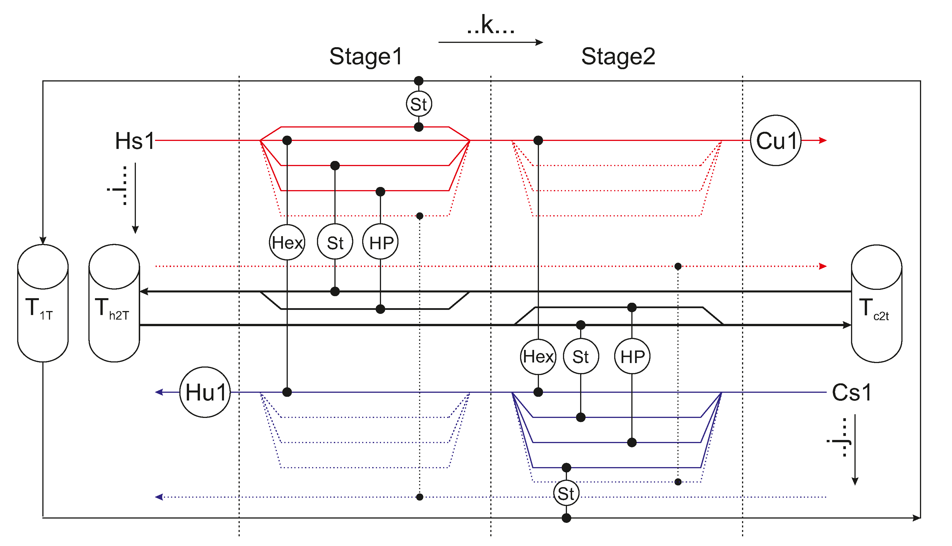
All test cases presented in Section 2 are optimized in two variations. In the first variation, which in the following is referred to as traditional HEN, only HEX between the streams and utilities are permitted in order to create a basic multi-period HEN in the traditional sense by setting all binary variables for the existence of $Z_{hp}$) and the existence of ST ($Z_{st}$ (HP) to zero. In the second, the integration of the possible ST and HP options in the extended superstructure formulation given in Appendix A is enabled. The optimization results are described in the following Section 3.1.1 to Section 3.1.4 and summarized discussed in Section 3.2.

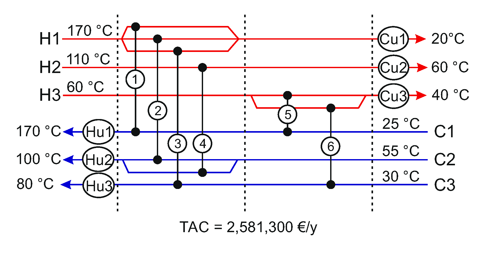
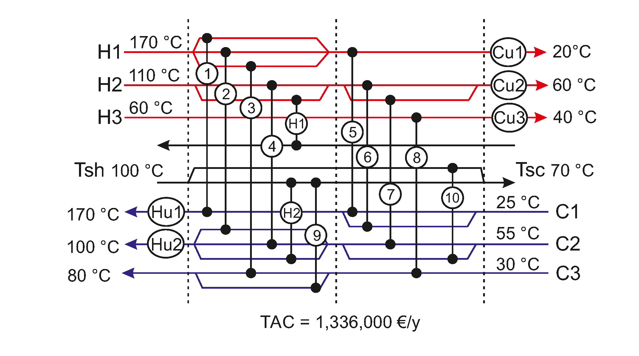
3.1.1. Results Case 1

In

Table 5. Heat Flows without HP and ST case 1 (kW).

Installation	p1	p2	p3	p4
1	1005.3	1425.4	-	3340.8
2	994.7	129.2	1000	659.2
3	1400	350	1555.8	350
4	1355.3	1420.8	1350	890.8
5	500	895.5	444.2	1650
6	3000	600	3000	600
7	1400	1000	1400	1000
8	244.7	179.2	250	709.2
Cu1	-	2445.5	-	-
Cu2	100	754.5	-	-
Hu1	-	-	1055.8	1800
Hu2	-	-	3344.2	-

and

Table 6. Heat Flows and $P_{el}$ results with HP and ST options case 1 (kW).

Installation	p1	p2	p3	p4
1	-	-	-	3150
2	-	-	497.5	250
3	825.1	2000	-	1884.1
4	-	-	488.1	-
5	906.5	1100	906.5	-
6	425.1	350	502.5	100
7	974.9	-	1800	-
8	3000	600	3000	600
9	1400	1000	1400	100
10	693.5	500	205.3	1600
11	920.4	474.4	-	200
12	-	-	1732.1	-
13	1443.5	450	1443.5	1500
14	654.5	3175.6	-	300
15	231.5	-	566.5	865.9
Cu1	200	-	200	115.9
Hu1	-	-	490	-
Hu2	-	-	367.9	-

, the heat flows of the HEN solutions for case 1 in Figure 2 and Figure 3 are given. The traditional HEN solution consists of eight stream - stream HEX and four utility HEX and has total annual costs of $TAC=2,999,100$ €$y^{-1}$. The utilities for periods 1 to 4 for this case fit exactly to the minimum utility demand calculated in Section 2.1, which means that within the single periods, the maximum possible energy recovery is obtained.

The extended HEN consists of ten streams, stream HEX, five streams, ST HEX, three utility HEX, and two storages, and has total annual costs of $TAC=1,336,700$ €$y^{-1}$. The chosen 1T ST operates between 100 °C and 183 °C and the 2T ST has a optimized size of $m_{StC1}=155,887$ kg.

3.1.2. Results Case 2

In

Table 7. Heat Flows without HP and ST case 2 (kW).

Installation	p1	p2	p3	p4
1	1260	660	924.4	1260
2	-	180	-	-
3	-	150	250	-
4	800	1600	900	800
5	-	180	195.6	-
Cu1	90	360	625.6	90
Cu2	-	-	1100	-
Cu3	20	190	954.4	-
Hu1	915	30	40	1350
Hu2	100	20	-	550
Hu3	500	-	-	680

and

Table 8. Heat Flows and $P_{el}$ results with HP and ST options case 2 (kW).

Installation	p1	p2	p3	p4
1	596.3	594.7	700.3	540
2	-	147.4	350.2	-
3	-	150	-	-
4	100	-	350.6	-
5	633.8	245.3	419.7	698.8
6	442.5	-	-	741.2
7	257.5	227.1	199.2	-
8	500	150	250	520
9	500	0	250	680
10	542.5	-	-	-
Cu1	90	212.6	329.8	111.2
Cu2	-	89.2	199.2	58.8
Cu3	20	370	1150	-
Hu1	472.5	30	40	630
Hu2	-	-	-	36.6
HP1	-	1283.7	1251	-
HP2	-	1425.6	-	1313.4
Pel HP1	-	638.3	625.5	-
Pel HP2	-	475.2	-	437.8

, the heat flows of the HEN solutions for case 2 in Figure 4 and Figure 5 are given. The traditional HEN solution consists of five stream - stream HEX and six utility HEX and has total annual costs of $TAC=2,581,300$ €$y^{-1}$. That Hu and Cu are necessary within the same time periods show that the theoretical minimum utility demand is not reachable, or at least not financial desirable for this case.

The extended HEN consists of eight stream - stream HEX, two stream—ST HEX, five utility HEX, two HP, and a 2T ST and has total annual costs of $TAC=1,336,000$ €$y^{-1}$. The 2T ST has a optimized size of $m_{StC2}=490,601$ kg and the HP have a maximum electrical power consumption of $P_{elHP1}=638.3$ kW and $P_{elHP2}=475.2$ kW, respectively.

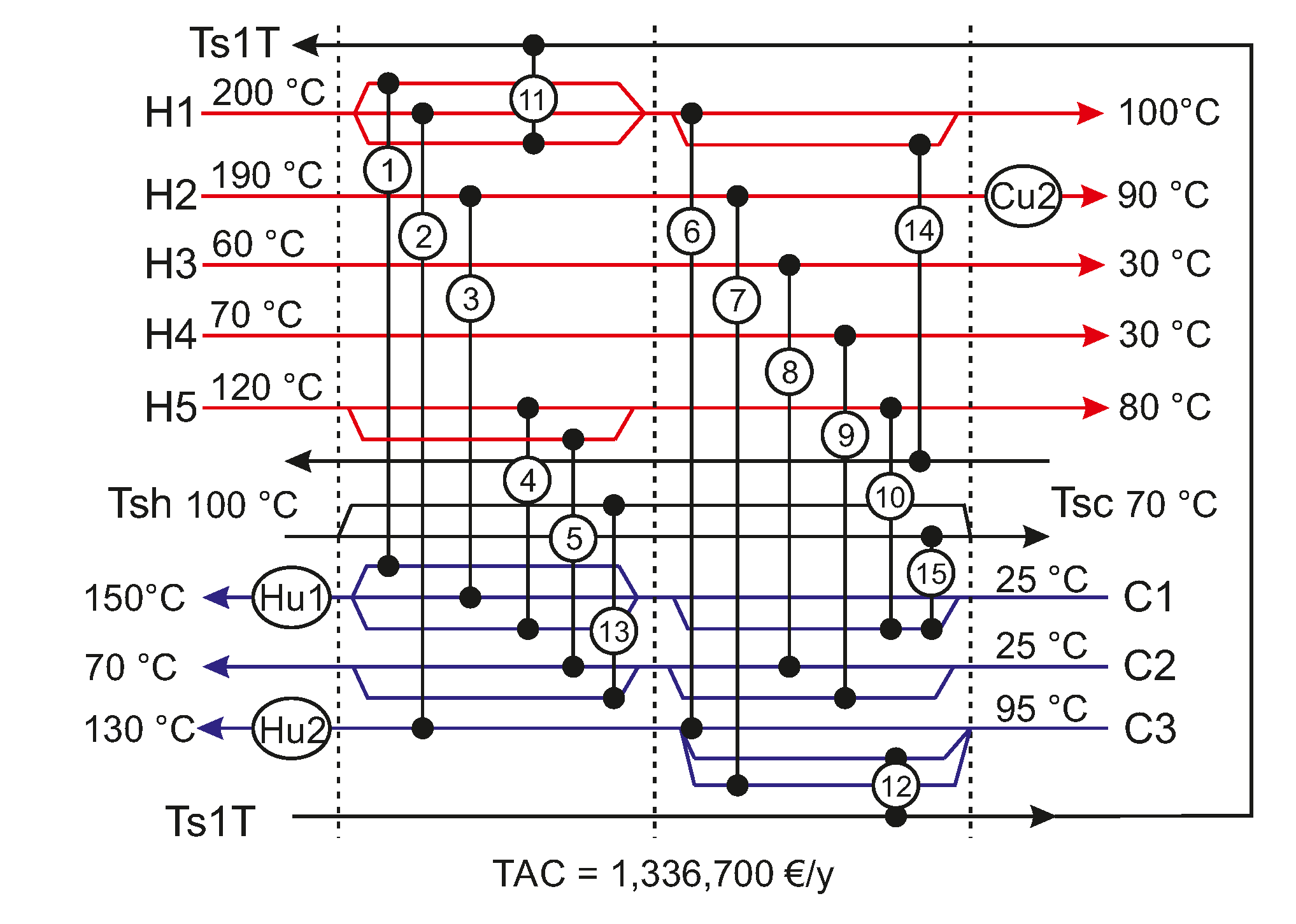
3.1.3. Results Case 3

In

Table 9. Heat Flows without HP and ST case 3 (kW).

Installation	p1	p2	p3	p4
1	-	-	229.7	518.3
2	4467.8	2259.8	4900	-
3	-	2100	-	-
4	1874	1598.8	2345.5	3398.6
5	556.6	592.8	120.8	373.1
6	2800	2800	2800	2800
7	180.2	209.8	170.3	481.7
8	569.8	540.2	-	-
9	3782.2	3879.8	3350	-
10	763.7	911.7	734.2	728.4
11	705.7	757.2	699.5	-
Cu1	250	250	-	-
Cu2	-	3010.5	-	75
Cu3	600	639.5	600	-
Hu1	-	-	-	1991.4
Hu2	162.3	-	200	2400
Hu3	-	-	-	1400
Hu4	87.7	-	300	458.6

and

Table 10. Heat Flows and $P_{el}$ results with HP and ST options case 3 (kW).

Installation	p1	p2	p3	p4
1	2728.3	2384.9	3021.5	-
2	-	2100	-	-
3	1605.4	1688.4	1605.4	2519.5
4	587.8	509.8	587.8	765.4
5	2800	2800	2800	2800
6	750	514.1	300	750
7	4050	4494.1	4050	-
8	944.6	417.5	944.6	1215.2
9	762.2	840.2	762.2	-
10	-	-	-	584.6
Cu1	250	584.9	100	250
Cu2	-	895.4	-	75
Cu3	600	1044.1	600	-
HP1	1471.7	1375.6	1178.5	-
HP2	-	-	-	2865.4
HP3	1721.7	-	1878.5	1650
HP4	-	-	-	1400
Pel HP1	665.5	649.3	574.6	-
Pel HP2	-	-	-	637.8
Pel HP3	552.8	-	597.3	532.4
Pel HP4	-	-	-	424.6

, the heat flows of the HEN solutions for case 3 in Figure 6 and Figure 7 are given. The traditional HEN solution consists of eleven stream - stream HEX and seven utility HEX and has total annual costs of $TAC=3,594,800$ €$y^{-1}$. As for case 2, the theoretical minimum utility demand is not reachable, or at least not financial desirable for this case.

The extended HEN consists of nine stream, stream HEX, one stream, ST HEX, three utility HEX, four HP, and a 2T ST and has total annual costs of $TAC=1,880,200$ €$y^{-1}$. The 2T ST has a optimized size of $m_{StC3}=294,312$ kg and the HP have a maximum electrical power consumption of $P_{elHP1}=665.5$ kW, $P_{elHP2}=637.8$ kW, $P_{elHP3}=597.3$ kW, and $P_{elHP4}=424.6$ kW, respectively.

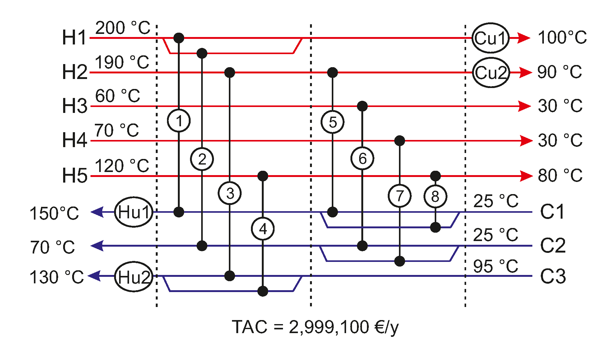
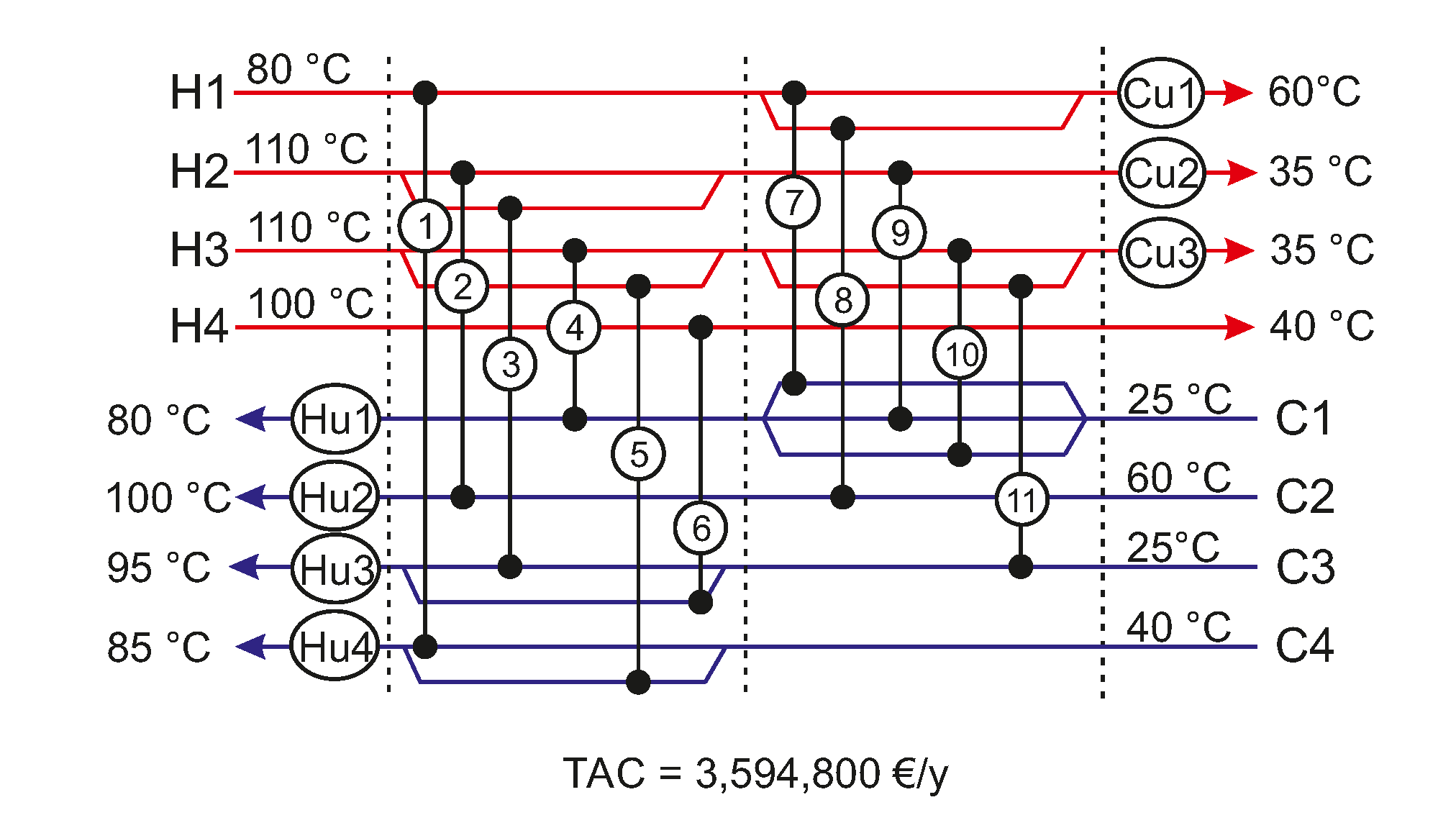
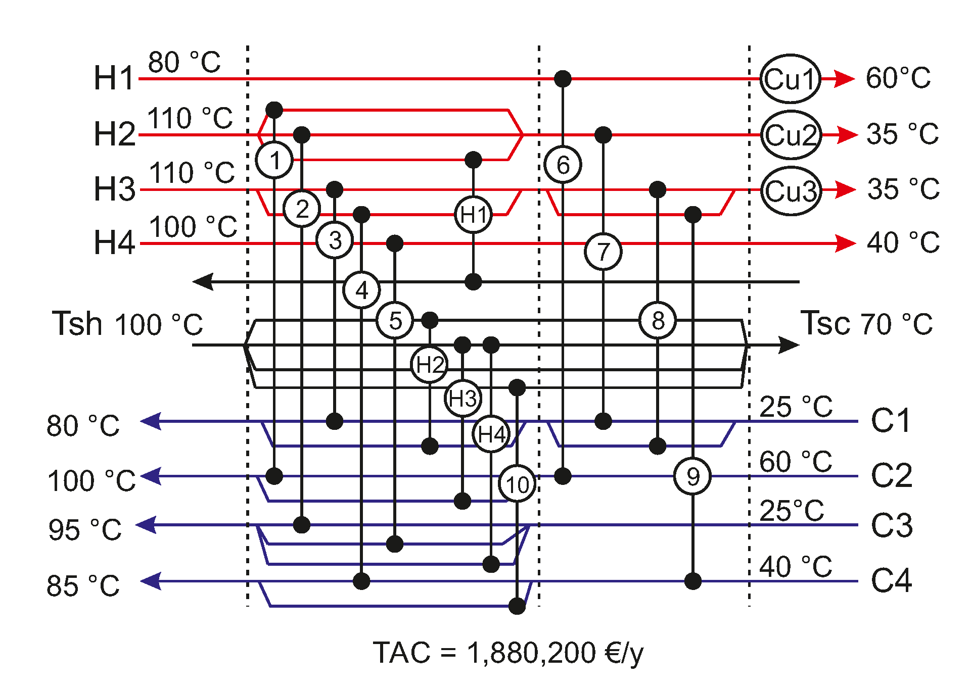
3.1.4. Results Case 4

In

Table 11. Heat Flows without HP and ST case 4 (kW).

Installation	p1	p2	p3
1	1000	-	1000
2	326.7	1571.1	-
3	1000	822.1	-
4	1805.6	279.32	902.4
5	2444.4	2040	117.6
6	840	371.1	960
7	-	1128.9	-
8	1373.3	1206.8	1200
9	-	308.9	-
10	2600	2777.9	780
Cu1	360	1800	240
Cu2	900	1380	600
Hu1	350	-	740
Hu2	473.3	-	1100
Hu3	821.1	-	1897.6
Hu4	1155.6	120	1322.4
Hu5	200	200	2070

and

Table 12. Heat Flows and $P_{el}$ results with HP and ST options case 4 (kW).

Installation	p1	p2	p3
1	471.1	-	471.1
2	143.2	1600	-
3	-	1871.1	-
4	3400	2040	1020
5	1190	680	1173.4
6	770	2000	775.7
7	1800	839.7	-
8	-	-	526.6
9	285.7	1160.3	728.9
Cu1	240	620	250.8
Cu2	2088.4	2541.4	313.4
Hu1	1400	-	1400
Hu2	200	120	420
Hu3	668.8	200	576.4
HP1	-	1860.3	2100
HP2	2218	-	1497.8
HP3	2261.6	2847.6	-
HP4	2128.9	2128.9	-
Pel HP1	-	400	456.7
Pel HP2	739.3	-	499.3
Pel HP3	1130.8	1423.8	-
Pel HP4	709.6	709.6	-

, the heat flows of the HEN solutions for case 4 in Figure 8 and Figure 9 are given. The traditional HEN solution consists of ten stream - stream HEX and seven utility HEX and has total annual costs of $TAC=7,160,800$ €$y^{-1}$. The large Hu and Cu needed within the same time periods show that the temperature levels and heat capacities of the streams do not allow a heat recovery near the theoretical optimum calculated in Section 2.4.

The extended HEN consists of eight stream, stream HEX, one stream, ST HEX, five utility HEX, four HP, and a 2T ST and has total annual costs of $TAC=5,056,600$ €$y^{-1}$. The 2T ST has a optimized size of $m_{StC4}=199,932$ kg and the HP have a maximum electrical power consumption of $P_{elHP1}=456.7$ kW, $P_{elHP2}=739.3$ kW, $P_{elHP3}=1423.8$ kW, and $P_{elHP4}=709.6$ kW, respectively.

3.2. Discussion

The summarized results of the optimization of the four cases are given in

Table 13. Summary of optimization results.

Case	TAC	Utilities/Year	Pel/Year	Energy Demand/Year	Installations	Storage
	€${\mathbf{y}}^{-1}$	GWh ${\mathbf{y}}^{-1}$	GWh ${\mathbf{y}}^{-1}$	GWh ${\mathbf{y}}^{-1}$	-
1	2,999,100	21.93	-	21.93	12
1 extended	1,336,700	2.829	-	2.829	20	1T, 2T
2	2,281,300	16.37	-	16.37	12
2 extended	1,336,000	8.256	4.680	12.94	18	2T
3	3,594,800	21.25	-	21.25	18
3 extended	1,880,200	8.527	10.07	18.59	18	2T
4	7,160,800	45.09	-	45.09	17
4 extended	5,056,600	31.66	19.43	51.09	19	2T

, where it can be seen that for all cases, the integration of HP and ST into the HEN significantly reduced the TAC. The TAC of case 1 were reduced by $1,662,400$ €$y^{-1}$ or 55.43%, the TAC of case 2 were reduced by $945,300$ €$y^{-1}$ or 41.43%, the TAC of case 3 were reduced by $1,714,600$ €$y^{-1}$ or 47.70% and the TAC of case 4 were reduced by $2,104,200$ €$y^{-1}$ or 29.39%. The total external energy demand for cases 1-3 decreased by 87.10%, 20.95%, and 12.52%, respectively, while the total external energy demand of case 4 increased by 13.31%. Except for case 3, all extended HEN consist of more installations than their basic HEN counterpart.

For case 1, the significant reduction of the utility energy demand is caused by the optimal integration of the two different possible ST options. This is possible because the 1T ST has a fixed size and the operational temperatures are chosen during the optimization while for the 2T ST the temperature levels of the tanks are fixed and the size gets optimized. Thanks to this combination, the optimized storages allow to shift the heat surplus from period 2 mentioned in Section 2.1 to periods 3 and 4. This reduces the overall Cu energy demand and the overall Hu energy demand for one cycle by 8884.1 kWh, which results in an annual reduction of utility costs of $2,101,111$ €$y^{-1}$ for the given cost coefficients.

The optimal integration of a 2T ST and two HP in case 2 led to a reduction of the Cu demand per cycle of 799.2 kWh and a reduction of the Hu demand per cycle of 2975.9 kWh. The electrical energy demand of the two HP per cycle is 2176.7 kWh, which shows that Hu demand is shifted towards electrical energy demand, which reduces the annual energy costs by $1,173,599$ €$y^{-1}$.

For case 3, the four HP and the 2T ST chosen by the optimization reduced the Cu demand per cycle by 925.6 kWh and led to a solution without Hu, thus decreasing the Hu demand by 7950 kWh. The Hu demand is replaced by the HP, which has an electrical energy demand per cycle of 7024.4 kWh, reducing the annual energy costs by $2,003,480$ €$y^{-1}$.

The integration of the 2T ST and the four HP in the resulting extended HEN of case 4 resulted in a higher annual external energy demand than the traditional HEN solution. The Cu demand increased by 774 kWh while the Hu demand was reduced by 5464.8 kWh. The electrical energy demand per cycle of the 4 HP combined adds up to 6778.7 kWh. While it may seem that an increased external energy demand is not an improvement, it must be remembered that the optimization target is the minimization of the TAC and only depends on the specific cost coefficients. Although in this case the external energy demand increased, the annual energy costs for the extended network solution are $2,003,480$ €$y^{-1}$ lower than for the traditional HEN solution. Even small changes of the cost parameters can result in massive changes in the resulting network solutions. Assuming that the electrical energy demand is satisfied through GHG neutral energy sources and that the Cu only needs electrical energy for transportation of the fluid, the generation of steam for the Hu remains the only GHG source during operation. With this assumption and the given case data and cost coefficients, the extended HEN solutions for cases 1 to 4 yield the theoretical potential for a drastic reduction of GHG emission of 83.8%, 71.1%, 100%, and 52.3% respectively.

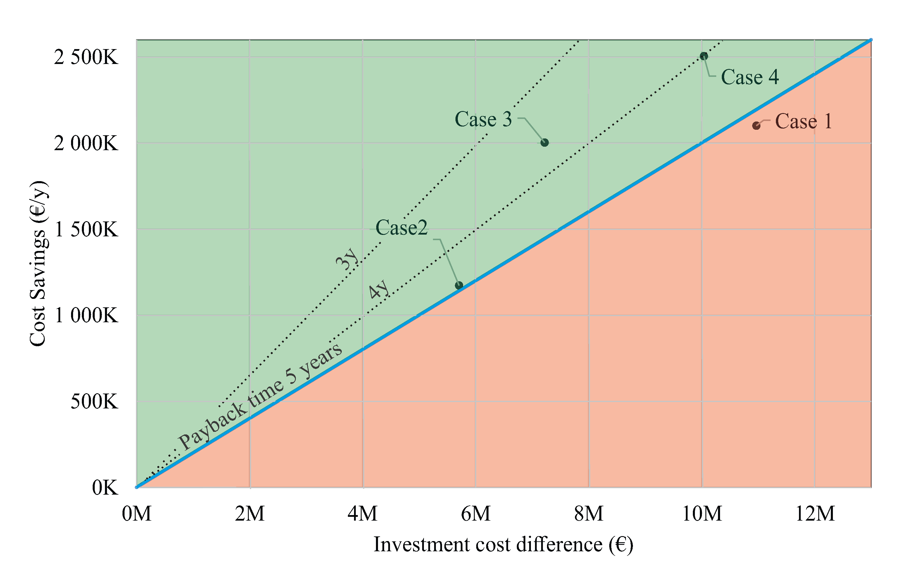
As mentioned in the introduction, energy-saving or emission reduction investments have to compete with other measures like capacity improvements. The payback time is often taken as an indicator to determine if a more expensive investment in an environmentally friendly alternative is profitable or not. For the proposed cases, the payback time for an assumed lifespan of 25 years is calculated by dividing the investment cost difference of the extended and the basic HEN results by the annual saving of energy costs. For visualization, the annual cost savings of the cases are given over their investment cost difference in Figure 10. The diagonal line in Figure 10 represents a payback time of five years, which is exemplary set as a realistic limit for the profitability of the investments. Regarding the extended HEN for case 1, a payback time of 5.2 years was obtained, making it not profitable under the assumptions given in Section 1.2 and Section 2. The payback times of cases 2–4, that are 4.9 years, 3.6 years, and 4.0 years, respectively, are within the limit and thus profitable investments. The fact that the payback times of the analyzed cases lay close to the profitability limit fits well with reality in the industry. The difficulty of achieving carbon neutrality without the influence of regulations or subsidies is highlighted in the results of case 1, where even an energy demand reduction of 87.10% by the introduced HEN can not be considered profitable from an economic point of view. The obtained results show that the introduced set of test cases with their different optimization potentials are perfectly suitable for extensive tests of multi-period HENS procedures under realistic conditions.

4. Conclusions

A set of four example cases suitable for HP and ST integration was created based on industrial processes from the EII to increase the small number of publicly available test cases in the field of multi-period HENS and to show the potential of energy integration in different sectors of the EII. The application of an approach that allows the simultaneous integration of HP and different types of ST presented in earlier work [3] led to a significant reduction of the total annual cost compared to the basic HEN of up to 55.43% for the introduced cases. Moreover, the external energy demand was reduced (up to 87.1%), or shifted towards possible renewable energy sources. These results are perfectly plausible considering the chosen cost coefficients and the structure of the cost function. Within the taken assumptions, three of the four extended HEN results have payback times under five years and are thus potential profitable investments. The results underline the potential of design optimization in the reduction of CO₂ emissions while also improving cost-efficiency, especially in the EII. While it is clear that the optimization of constructed test cases is not directly transferable to real applications, the introduced stream data combined with the results obtained and the fully given mathematical formulation provide a valuable extension to the existing HENS literature and contribute to future research in the field.

References

1. European Commission. Statistical Office of the European Union. Energy Balance Sheets: 2020 Edition; Publications Office: Singapore, 2020. [Google Scholar] [CrossRef]
2. de Bruyn, S.; Jongsma, C.; Kampman, B.; Görlach, B.; Thie, J.E. Energy-Intensive Industries: Challenges and Opportunities in Energy Transition; European Parliament: Region de Bruxelles-Capitale, Belgium, 2020. [Google Scholar] [CrossRef]
3. Prendl, L.; Schenzel, K.; Hofmann, R. Simultaneous integration of heat pumps and different thermal energy storages into a tightened multi-period MILP HENS superstructure formulation for industrial applications. Comput. Chem. Eng. 2021, 147, 107237. [Google Scholar] [CrossRef]
4. Rathjens, M.; Fieg, G. Cost-Optimal Heat Exchanger Network Synthesis Based on a Flexible Cost Functions Framework. Energies 2019, 12, 784. [Google Scholar] [CrossRef] [Green Version]
5. Jegla, Z.; Freisleben, V. Practical Energy Retrofit of Heat Exchanger Network Not Containing Utility Path. Energies 2020, 13, 2711. [Google Scholar] [CrossRef]
6. Wang, B.; Klemeš, J.J.; Varbanov, P.S.; Zeng, M. An Extended Grid Diagram for Heat Exchanger Network Retrofit Considering Heat Exchanger Types. Energies 2020, 13, 2656. [Google Scholar] [CrossRef]
7. Escobar, M.; Trierweiler, J.O. Optimal heat exchanger network synthesis: A case study comparison. Appl. Therm. Eng. 2013, 51, 801–826. [Google Scholar] [CrossRef]
8. Soršak, A.; Kravanja, Z. MINLP retrofit of heat exchanger networks comprising different exchanger types. Comput. Chem. Eng. 2004, 28, 235–251. [Google Scholar] [CrossRef]
9. Papoulias, S.A.; Grossmann, I.E. A structural optimization approach in process synthesis—II. Comput. Chem. Eng. 1983, 7, 707–721. [Google Scholar] [CrossRef]
10. Floudas, C.A.; Grossmann, I.E. Automatic generation of multiperiod heat exchanger network configurations. Comput. Chem. Eng. 1987, 11, 123–142. [Google Scholar] [CrossRef]
11. Verheyen, W.; Zhang, N. Design of flexible heat exchanger network for multi-period operation. Chem. Eng. Sci. 2006, 61, 7730–7753. [Google Scholar] [CrossRef]
12. Stampfli, J.A.; Atkins, M.J.; Olsen, D.G.; Walmsley, M.R.; Wellig, B. Practical heat pump and storage integration into non-continuous processes: A hybrid approach utilizing insight based and nonlinear programming techniques. Energy 2019, 182, 236–253. [Google Scholar] [CrossRef]
13. Brown, H.L. Phase 1, industrial applications study. In Energy Analysis of 108 Industrial Processes; US Department of Energy: Philadelphia, PA, USA, 1979. [Google Scholar] [CrossRef]
14. Isafiade, A.; Bogataj, M.; Fraser, D.; Kravanja, Z. Optimal synthesis of heat exchanger networks for multi-period operations involving single and multiple utilities. Chem. Eng. Sci. 2015, 127, 175–188. [Google Scholar] [CrossRef]
15. Shen, L.; Worrell, E.; Patel, M.K. Environmental impact assessment of human-made cellulose fibres. Resour. Conserv. Recycl. 2010, 55, 260–274. [Google Scholar] [CrossRef]
16. Garcia-Herrero, I.; Margallo, M.; Laso, J.; Onandía, R.; Irabien, A.; Aldaco, R. Measuring the Vulnerability of an Energy Intensive Sector to the EU ETS under a Life Cycle Approach: The Case of the Chlor-Alkali Industry. Sustainability 2017, 9, 837. [Google Scholar] [CrossRef] [Green Version]
Figure 1. “Superstructure with possible Stream-Stream Hex (HEX), Stream-Storage Hex (ST) and Heat Pumps (HP)” from Prendl et al. [3]/CC BY 4.0.“Superstructure with possible Stream-Stream Hex (HEX), Stream-Storage Hex (ST) and Heat Pumps (HP)” from Prendl et al. [3]/CC BY 4.0.
Energies 14 06741 g001
Figure 2. HEN obtained without HP and ST options case 1.HEN obtained without HP and ST options case 1.
Energies 14 06741 g002
Figure 3. HEN obtained with HP and ST options case 1.HEN obtained with HP and ST options case 1.
Energies 14 06741 g003
Figure 4. HEN obtained without HP and ST options case 2.HEN obtained without HP and ST options case 2.
Energies 14 06741 g004
Figure 5. HEN obtained with HP and ST options case 2.HEN obtained with HP and ST options case 2.
Energies 14 06741 g005
Figure 6. HEN obtained without HP and ST options case 3.HEN obtained without HP and ST options case 3.
Energies 14 06741 g006
Figure 7. HEN obtained with HP and ST options case 3.HEN obtained with HP and ST options case 3.
Energies 14 06741 g007
Figure 8. HEN obtained without HP and ST options case 4.HEN obtained without HP and ST options case 4.
Energies 14 06741 g008
Figure 9. HEN obtained with HP and ST options case 4.HEN obtained with HP and ST options case 4.
Energies 14 06741 g009
Figure 10. Cost savings per year over investment cost difference between conventional HEN and extended HEN results. In the green area the payback time is shorter than 5 years and in the red area the payback time is longer than 5 years.Cost savings per year over investment cost difference between conventional HEN and extended HEN results. In the green area the payback time is shorter than 5 years and in the red area the payback time is longer than 5 years.
Energies 14 06741 g010