A Novel Methodology for Optimal SVC Location Considering N-1 Contingencies and Reactive Power Flows Reconfiguration

Abstract

In this research, an alternative methodology is proposed for the location of Static VAR Compensators (SVC) in power systems, considering the reconfiguration of reactive power flows through the optimal switching of the transmission stage, which resembles the contingency restriction N-1 usually considered in transmission expansion planning. Based on this methodology, the contingency index was determined, which made it possible to determine which is the contingency that generates the greatest voltage degradation in the system. For the quantification of reactive flows, optimal AC power flows were used, which minimize the operating costs of the power system subject to transmission line switching restrictions, line charge-ability, voltages and node angles. To determine the node in which the compensation should be placed, the contingency index criterion was used, verifying the voltage profile in the nodes. The proposed methodology was tested in the IEEE test systems of 9, 14 nodes and large-scale systems of 200, 500 and 2000 bus-bars; to verify that the proposed methodology is adequate, the stability of the EPS was verified. Finally, the model allows satisfactorily to determine the node in which the SVC is implemented and its compensation value.

1. Introduction

In electrical power systems (EPS) the use of technologies such as distributed generation (DG) and reactive compensation devices has increased considerably over time with the objective of improving voltage profiles in nodes, through this way it is also possible to improve the EPS general performance, obtaining results such as reduction of active and power losses, minimization of environmental pollution and maximization of the load that the system can support [1].

Reactive compensation devices known as FACTS (Flexible AC Transmission System) are power electronic converters that have the ability to control various electrical parameters, such as steady-state power flow and dynamic stability control [2]. Within FACTS devices, the most widely used within transmission networks is the static VAR compensator (SVC) due to its low cost, simplicity and good performance in the system, this device is connected in bypass in the different bars of the EPS in order to absorb or generate VAR, and the device output adjusts to improve capacitive or inductive current to control specific power electrical system parameters such as voltage profiles [3].

Flexible AC transmission systems (FACTS) are devices that have the ability to control various electrical parameters, such as steady state power flow and dynamic stability control [2]. In Electrical Power Systems, one of the most studied devices is the static VAR compensator (SVC); due to its low cost, simplicity and good performance in the system, this device is connected in derivation in the different bars of the system in order to absorb or generate reactive power (VAR), whose output is adjusted to improve the capacitive or inductive current and thus control specific parameters of the electrical power system such as voltage profiles [3].

The electrical transmission system is one of the most important stages for EPS operation, this stage is intermediate in the transfer of electrical energy from generation to distribution stages. As large power generation plants are installed, transmission networks are becoming more complex due to the increase in load and the dynamic load pattern that directly affects the transmission lines, where they are working under over-loaded or under-loaded conditions; this unevenness on electrical load directly affects the voltage profiles and makes the EPS safety vulnerable to faults, at the same time active and reactive power flow increases, producing loss of supplementary power and increasing voltage drops [4,5].

According to [5], traditional EPS planning and operation must be reformulated, because the conventional approach (adding new transmission lines in the system and building new power generation facilities) is subject to various factors, such as technical and economic limits; If consumer demand is high, transmission lines would operate near their maximum capacity or simply would be overloaded, causing power flows on the line to easily violate established ones, thus leading to voltage instability. Therefore, the best solution is to make optimal use of the existing generation and transmission network.

Voltage stability is the ability of an electrical power system to maintain bus bar voltages within accepted and established ranges, whether working under normal conditions or under disturbances. The implementation of FACTS is an alternative to improve EPS performance, instead of designing and installing new and complex transmission lines [6,7].

Stability analyzes in electrical power systems are focused on determining the limit conditions at which the EPS lose stability, conditions such as increased load, contingencies, among others. In [8] a methodology based on the bifurcation theorem known as Continuation Power Flow (CPF) is proposed in order to identify the weak nodes of the EPS by performing voltage stability analysis. Voltage stability studies based on CPF can be used for mesh systems such as transmission-generation systems, as well as for radial distribution systems and can use Newton Raphson (NR) or optimal power flows to determine the different electrical parameters of the system [9,10].

The insertion of SVC technology is highly effective because it prevents voltage instability, however, the performance and each of the benefits of these devices is directly linked to the location in which it will be placed and what capacity it will have because one of the limitations in the transmission stage of these devices generally originates from investment costs when implementing this type of technology in the transmission lines [11,12].

According to [13], the problems alleviated by FACTS are classified into two groups, as steady-state and transient stability problems. Steady-state problems have been subdivided into three sections such as voltage control, power system optimization, cost minimization, and contingency analysis. In the same way, transient stability problems have been subdivided into two sections, voltage stability and angular stability. In each case, the aim is to alleviate both instability and costs, as well as to reduce the effort of the network.

The optimal location of SVC according to the literature review is carried out using optimization techniques, heuristic and meta-heuristic techniques, genetic algorithms and techniques based on artificial intelligence [14,15,16], focusing on improving the voltage stability of the EPS and the concept of transfer capacity maximum power of the lines and node [17].

In [18], the optimal location is performed using the HPSO technique, which reduces generation costs, transmission losses and increases the generation capacity along with the power transfer capacity in the SEP; this work carries out its research on a 30-bus bar IEEE model using optimal power flows in the same way.

In [19], the optimal location of SVC is proposed based on the particle swarm optimization (PSO) model, in order to minimize the deviations of the voltage profiles in the bars and the losses that exist in the network.

Ref. [20] proposes an approach that relies on the sensitivity of the actual power flow performance index and the line interruption distribution factor to decide the optimal placement of FACTS as thyristor-controlled series compensators (TCSC) and Static Synchronous Series Compensators (SSSC) in order to improve stability and voltage profiles in a 30-bus bar IEEE model.

On the other hand, it must be taken into account that electrical power systems can operate very close to their limit conditions, which means that the models for analyzing power flows are not efficient and in many cases, they are unable to find the solution to the flow. The mathematical complexity that occurs in large-scale systems (>1000 buses) generates the need to apply alternative methodologies such as CPF, similar adverse conditions (ill-conditioned) can occur when contingencies are analyzed in the EPS [21,22]. In [23] a methodology is proposed to relax the mathematical complexity for the solution of OPF and optimal power flows with security restrictions (SOPF), in the document different contingency scenarios are analyzed and by means of a meta-heuristic the solution to infeasible problems is obtained with traditional methodologies.

One of the advantages of placing compensators in EPS is the reduction in the amount of reactive power (Mvar) that is transported by the transmission lines, making the active power (MW) that can be transferred from one node to another increase significantly, it also helps the voltage profile to be within acceptable limits. For the analysis of the behavior of the EPS in the present investigation, optimal AC power flows (OPF-AC) are used, with which it is possible to determine the behavior in steady-state before and after the implementation of reactive compensation. The present research focuses on determining the ideal point for the location of reactive compensation in EPS by studying the ranking of contingencies applied to the nodal voltage profiles considering contingency criteria N-1 and change in the EPS topology based on switching optimal transmission lines.

From now on the article is organized as follows: in Section 2 the theoretical support for the location of reactive compensation and optimal AC power flows is presented, in Section 3 the formulation of the problem is presented for later in Section 4 to analyze the main results obtained and finally, Section 5 shows the main conclusions of the research.

2. Electrical Power Systems Operation

Studies of the behavior in the operation of power systems can be carried out by means of different techniques, some being more demanding than others from the computational point of view. The most common are iterative techniques such as Gauss-Seidel and Newton Raphson, which allow a very rapid analysis of the steady-state behavior of the EPS. Techniques such as optimal power flows, make it possible to minimize EPS operating costs and maximize the use of its elements, considering technical and economic limits [24,25].

2.1. Optimal Power Flow AC (OPF-AC)

The OPF-AC allows determining the exact behaviour of the EPS, enabling to have an analysis of all the electrical parameters. OPF-AC seeks to minimize operating costs through  (1) and is subject to  (2) and  (3) that determine the balance of active and reactive power between generation, demand and power flow, through  (4) and  (5) that determine the flow of active and reactive power that circulates by a transmission line depending on its susceptance and conductance, in  (6) and  (7) the restrictions of active and reactive power limits of the generators are shown,  (8) delimits the voltages in each node and the limits of the angular difference in each branch is  (9) [26,27,28,29,30].

Objective Function:

$$minOF=\sum _{g=1}^{n_G}\left(a_g*S_g^2+b_g*S_g+c_g\right);\forall g\in n_G$$

(1)

Subject to:

$$P_g-P_D=\sum _{i=1}^{n_{bus}}{P}_{i}j;\forall i,j\in n_{bus}$$

(2)

$$Q_g-Q_D=\sum _{i=1}^{n_{bus}}{Q}_{i}j;\forall i,j\in n_{bus}$$

(3)

$$P_{ij}={\left|V_i\right|}^2{G}_{ij}-\left|V_i\right|\left|V_j\right|\left[G_{ij}cos\left({\delta }_i-{\delta }_j\right)+B_{ij}sin\left({\delta }_i-{\delta }_j\right)\right];\forall i,j\in n_{bus}$$

(4)

$$Q_{ij}={\left|V_i\right|}^2{G}_{ij}-\left|V_i\right|\left|V_j\right|\left[G_{ij}sin\left({\delta }_i-{\delta }_j\right)+B_{ij}cos\left({\delta }_i-{\delta }_j\right)\right];\forall i,j\in n_{bus}$$

(5)

$$P_g^{min}⩽P_g⩽P_g^{max};\forall g\in n_G$$

(6)

$$Q_g^{min}⩽Q_g⩽Q_g^{max};\forall g\in n_G$$

(7)

$$\left|V_i^{min}\right|⩽\left|V_i\right|⩽\left|V_i^{max}\right|;\forall i\in n_{bus}$$

(8)

$${\delta }_{ij}^{min}⩽{\delta }_{ij}⩽{\delta }_{ij}^{max};\forall i,j\in n_{bus}$$

(9)

2.2. Optimal Transmission Switching (OTS)

The switching of transmission lines (OTS) in power systems has been studied since its application in 2008 by Emily Fisher [31], who used the optimal DC power flows (OPF-DC) as the basis of the model. OTS allows alleviating the stress of the power system in situations of overload or atypical demands compared to the initial planning. OTS is a technique that allows maintaining the operation of the EPS, considering that the reliability may vary, since the operating parameters and the topology of the EPS change, likewise the point of stability of the system can change, but the use of OTS in case of any contingency is an alternative to avoid disconnections of distribution systems and end-users [32,33,34,35,36].

The authors in [37] modified the proposed OTS methodology so that it can be applied in the event of a contingency in the transmission systems; in which there is already talk of a reconfiguration of power flows in the face of contingencies seeking to maximize reliability.

OTS uses the OPF-AC mathematical model formulated in  (1)–(9) as a basis, this model increases the restrictions of the lines that can go out of operation by analyzing their chargeability  (10)–(15); the maximum number of switched lines is defined by (16) and in (17) it is shown the maximum power that can be switched in the EPS.

$$P_{ij}-B_{ij}*\left({\delta }_i-{\delta }_j\right)⩽\left(1-{\phi }_{ij}\right)*ML$$

(10)

$$P_{ij}-B_{ij}*\left({\delta }_i-{\delta }_j\right)⩾\left(1-{\phi }_{ij}\right)*ML$$

(11)

$$Q_{ij}-B_{ij}*\left({\delta }_i-{\delta }_j\right)⩽\left(1-{\phi }_{ij}\right)*ML$$

(12)

$$Q_{ij}-B_{ij}*\left({\delta }_i-{\delta }_j\right)⩾\left(1-{\phi }_{ij}\right)*ML$$

(13)

$${\phi }_{ij}*P_{ij}^{min}⩽P_{ij}⩽{\phi }_{ij}*P_{ij}^{max}$$

(14)

$${\phi }_{ij}*Q_{ij}^{min}⩽Q_{ij}⩽{\phi }_{ij}*Q_{ij}^{max}$$

(15)

$$\sum _{ij}\left(1-{\phi }_{ij}\right)⩽NSL$$

(16)

$$ML=max\left\{B_{ij}*\left({\delta }_i-{\delta }_j\right)\right\}$$

(17)

2.3. Contingencies Ranking

When contingencies occur in electrical power systems, all electrical parameters are altered and therefore the operation and expansion planners consider contingency scenarios N-1, therefore it is important to quantify the severity of the contingencies, which is why can do by (18).

$$J=\sum _{i=1}^n\left(\frac{W_i}{2m}*{\left(\frac{f_i}{f_{i_{max}}}\right)}^{2}m\right)$$

(18)

The value of the contingency index makes it possible to generate a ranking with which to identify which is the element most affected by the analysis of contingencies N-1 in a global way, this parameter will have different values for each electrical variable of the EPS.

3. Problem Formulation

The proposed methodology for the optimal location of parallel compensators type SVC is based on OPF-AC considering N-1 contingencies and reconfiguration of the EPS topology through OTS, with which the most sensitive node of the electrical system is determined against the different scenarios of contingencies by studying the contingency index, considering that $m=1$ and $W_i=1$ in such a way that all contingencies will have the same severity.

The generation of contingencies is done considering that from the point of view of the operational planning of the EPS, the formation of islands and schemes for the separation of areas should be avoided, resources must be optimized and massive degradation of the system should be avoided, for this purpose, the contingencies scenarios to be analyzed will be randomized throughout a selection based on a brute force scheme of selection of links between the nodes, but only one link at a time.

In order to test the proposed methodology, the IEEE 9 and 14 bus bar test systems will be used, in which the contingency index analysis will be performed by comparing the nodal voltage values obtained in each case of contingencies with the normal operating scenario in steady-state, by  (19). For the study, an over and under-voltage limit established by ks is considered, which can take values of ± 5% o ± 10%.

$$J=\frac{1}{2}\sum _{i=1}^{n_{bus}}{\left(\frac{V_i}{ks}\right)}^2$$

(19)

Algorithm 1 shows the proposed heuristic for optimal SVC location based on OPF-AC, OTS and N-1 contingencies. In step 1 the entry of the variables and connectivity parameters of the EPS is contemplated so that in step 2 the initial conditions of the EPS are evaluated through OPF-AC and through this process, the contingency index of the normal operating state is obtained. Then, in step 3, the contingency index N-1, OTS for each contingency is analyzed and compared with the one obtained in a normal operating state, through this comparison it is determined which is the node that presents the greatest degradation of the profile tension in the EPS. In step 4, once the node with the greatest degradation of the voltage profile has been determined, the capacity of the SVC is dimensioned in such a way that the contingency index is corrected and it is improved compared to the case of normal operation and considering OTS, in step 5, the system stability is verified through a multi-machine analysis of the angle of the generators, comparing the before and after of the implementation of the parallel compensation considering the contingency criterion N-1 that represents a transitory event in the EPS and in the same way, the behavior of the PV curve is verified at the node where the compensation is implemented. and then finally in step 6, the results of the proposed methodology are shown.

Algorithm 1 Heuristics for optimal SVC location.

Step: 1 Input data EPS parameterization Generator, lines, transformers, loads, connectivity matrix Step: 2 Determination of initial conditions OPF-AC $P_{ij},Q_{ij},V_i$ $J_{ori}=\frac{1}{2}{\sum }_{i=1}^{n_{bus}}{\left(\frac{V_i}{ks}\right)}^2$ Step: 3 Determination of J for N-1 contingencies for $i=1:n;n\in nodes$  for $j=1:n$   if $C_{ij}=1$     $C_{ij}=0$     $OPF-AC+OTS$      $J_k=\frac{1}{2}{\sum }_{i=1}^{n_{bus}}{\left(\frac{V_i}{ks}\right)}^2$      $C_{ij}=1$      $k=k+1$   end if  end for end for for $k=1:m;m\in Contingencies$  if $J_{ori}>J_k$    $J_{ori}=J_k$    $node=k$  end if end for Step: 4 Compensation using SVC Locate SVC in node $VA{R}_{SVC}=2.5$ while $V_i⩽ks$   $VA{R}_{SVC}=VA{R}_{SVC}+2.5$ end while Step: 5 Stability check $P{e}_i\left(t\right)={\left|V_i\right|}^2*G_{ii}+{\sum }_{i=1}^n\left|V_i\right|\left|V_j\right|Y_{ij}cos({\delta }_i\left(t\right)-{\delta }_j\left(t\right)-{\theta }_{ij})$ ${\omega }_{r_g}\left(t\right)={\omega }_{r_i}(t-\Delta t)+\frac{\Delta t*{\omega }_b}{4H_g}\left[2P{m}_g-P{e}_g\left(t\right)-P{e}_g(t-\Delta t)\right]$ ${\delta }_g\left(t\right)=-\frac{\Delta t^2{\omega }_{b}P{e}_g\left(t\right)}{8H_g}+{\alpha }_g\left(t-\Delta t\right)$ if ${\delta }_g\left(t\right)\in \left[{\delta }_{ij}^{min};{\delta }_{ij}^{max}\right]$   Go to step 6 else   Discard current location node   Go to step 3 end if Step: 6 Show results $node,VA{R}_{SVC},P_{ij},Q_{ij},V_i$

4. Results Analysis

The simulation was developed on a computer with an Intel (R) Xeon (R) CPU E3-1535 M v5 @ 2.90 GHz processor with 64 GB of RAM, as software, Matlab was used for modelling, GAMS for optimization and Digsilent Power Factory for simulation. When considering the switching of transmission lines based on OPF-AC as part of the model and being a non-linear model, CONOPT was used as a solver for optimization.

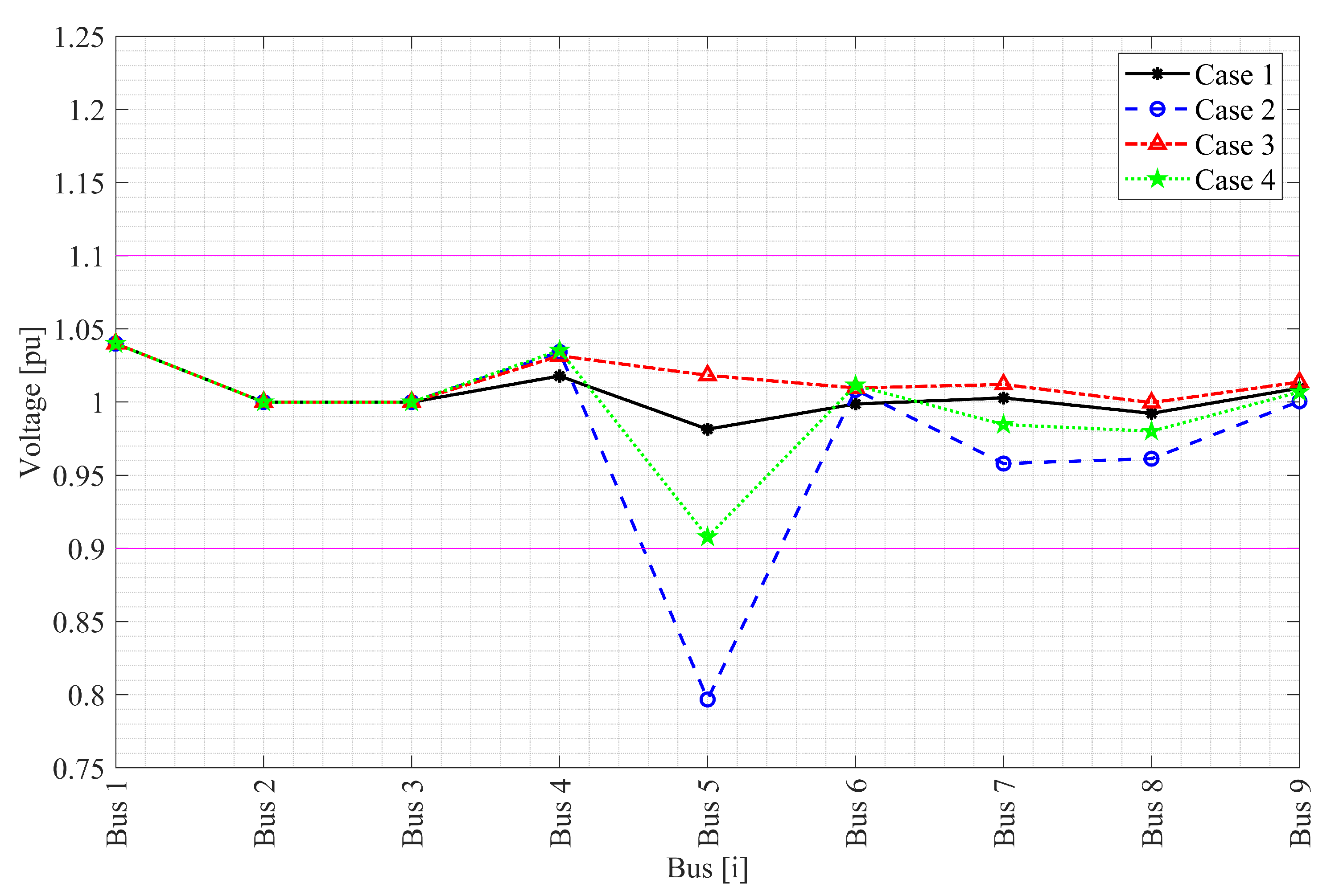
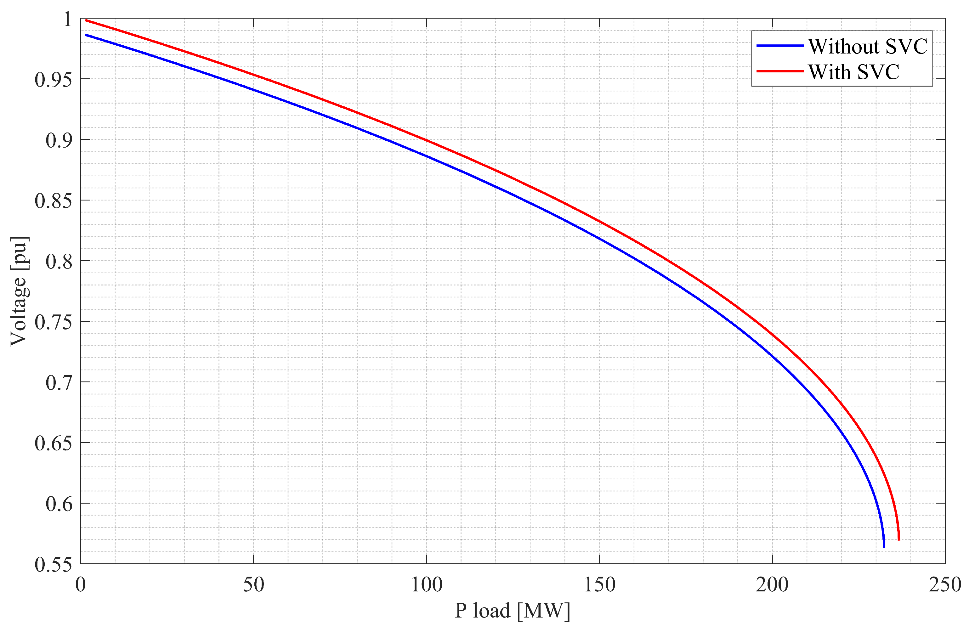
4.1. IEEE 9-Bus Bar Test System

Table 1. Contingency index of the IEEE 9-bus bar model.

Contingency	Without Compensation	With Compensation
Normal	3.7553	3.8237
Line 4–5	3.5727	3.6962
Line 5–7	3.6272	3.7140
Line 7–8	3.6553	3.7213
Line 8–9	3.7017	3.7726
Line 9–6	3.6577	3.7306
Line 6–4	3.6654	3.7273

contains the contingency index values in each of the simulated conditions, in the case of normal operation and in the event of an N-1 contingency, based on this, it is determined that the contingency that has the greatest impact on the EPS is when the line between nodes 4 and 5 fails and thereby verifying which node has the greatest voltage degradation, which is node 5 (Figure 1). Based on this analysis, the parallel compensation is located at node 5 and when applying the proposed methodology, the compensation that allows the voltage level at node 5 to be at least 0.9 p.u. is 40 Mvar, considering ks = ±10%. By placing this compensation value, the behavior of the system is checked again, having an improvement in the system’s voltage profile in the event of contingencies N-1. In the same way, the contingency index improves in this new scenario, without ceasing to be the worst contingency is the departure of line (4–5).

In Figure 2, the voltage behavior in each node is shown in the worst scenario determined by the contingency index, which corresponds to line (4–5). Case 1 represents the behavior of the EPS in a normal operating state without contingencies or compensation; in case 2, voltage response under a contingency in line (4–5) is shown and it is presented that node 5 is the worst voltage profile with a 0.7967 pu value. Case 3 corresponds to the response of the system after placing compensation (40 Mvar) in node 5 and in case 4 the response of the nodal voltage under the disconnection of the line (4–5) is shown, in which the voltage of node 5 was improved to 0.9078, thus complying with the proposed minimum voltage restriction.

The active power flows through the transmission lines are shown in Figure 3, in which it can be seen that the system requirements have small differences in the different scenarios analyzed, but no significant changes. On the other hand, the reactive flows in the transmission lines have a reconfiguration in the zone of incidence of node 5, with which there is a change in reactive flows in lines (4–5) and (5–7), in the other lines the changes are not very significant, as it can be seen in Figure 4.

Due to the simplicity of the IEEE 9-bus bar system, the effects on stability are minimal, as shown in Figure 5 when implementing the SVC in the system at node 5, it improves the load-increasing capacity at the node.

The transient response of the generators can be seen in Figure 6, which shows that the angles of the generators are kept within the established limits and without presenting severe changes, based on this it can be stated that the implementation of the SVC at node 5, apart from improving the voltage profile, it helps to maintain the EPS operation in a stable state in the presence of a contingency, which for the case study is line 4–5.

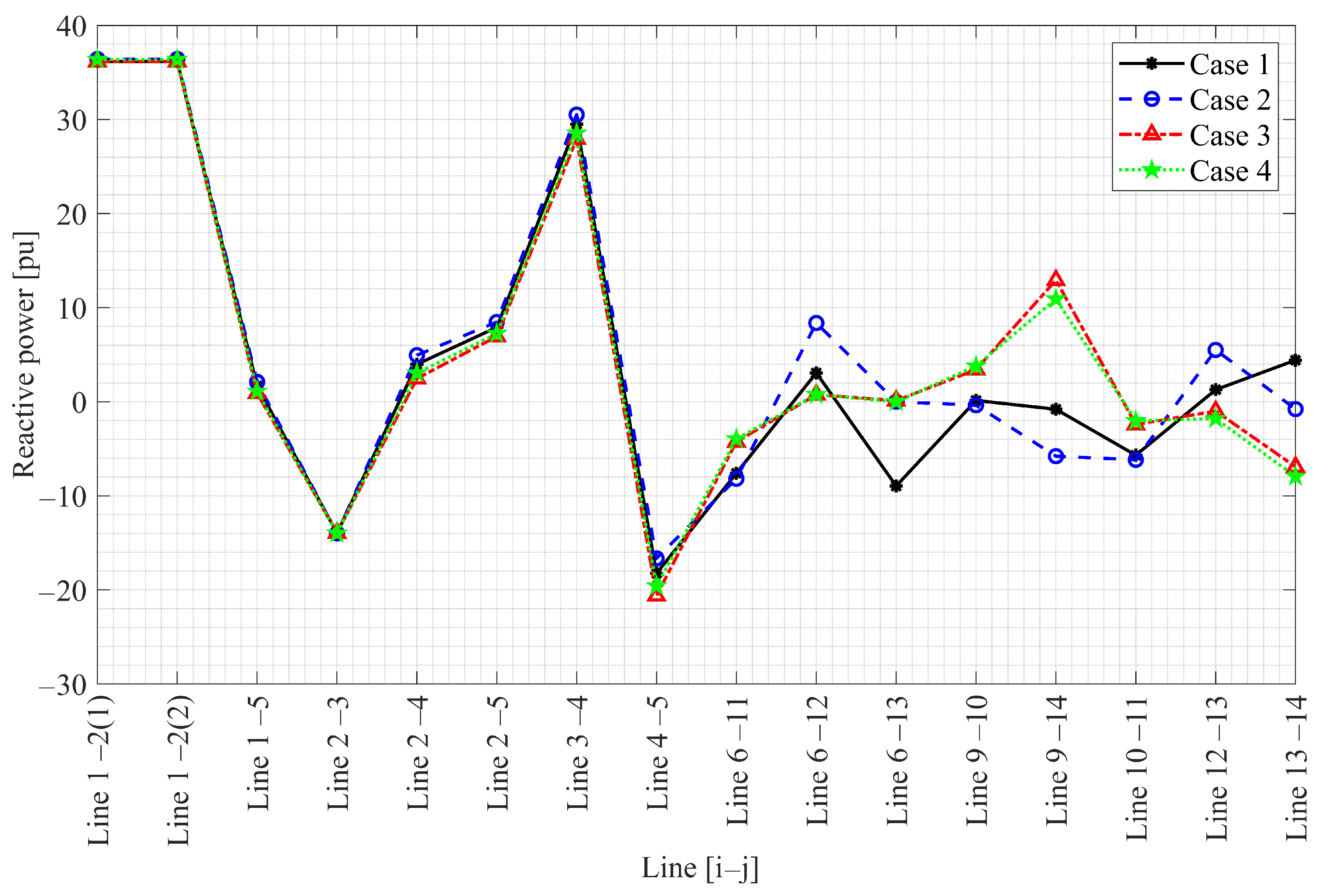
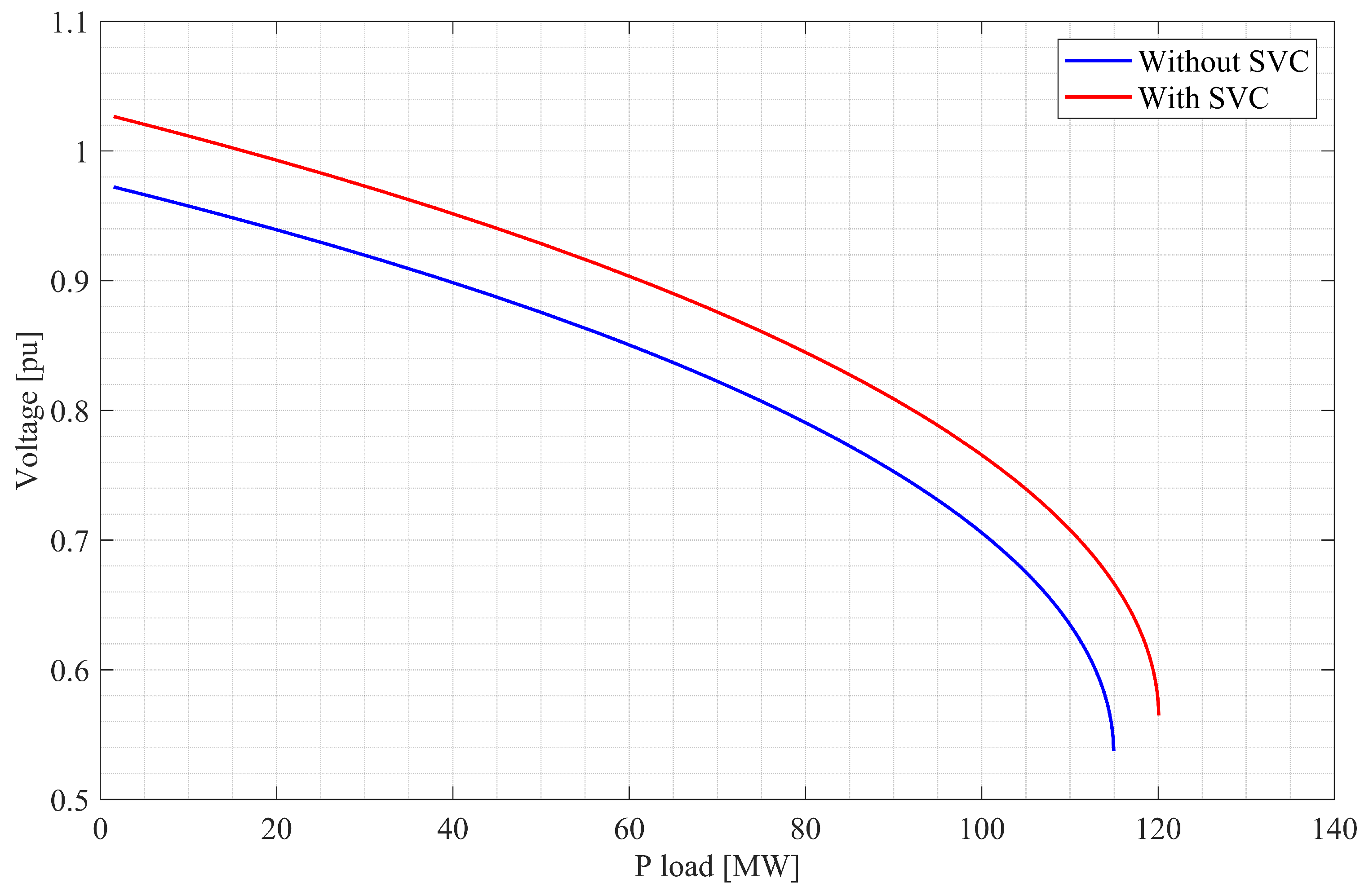
4.2. IEEE 14 Bus Bar Test System

The operational and connectivity characteristics of the IEEE 14-bus bar system allow this research to conduct the study and verify the applicability of the proposed methodology in any power system. Figure 7 shows the IEEE 14-bar model, in which the optimal location of reactive compensation is located at node 14 considering $ks=\pm 5\%$, with which the worst contingency index occurs when there is a fault on the line (6–13).

Based on the above, the next step is to determine the appropriate reactive compensation value, which allows a voltage value of at least 0.95 p.u. in nodes 13 and 14, this scenario was selected because it has a low voltage for the worst contingency. The compensation required to improve the voltage profile is 25 Mvar, with which the voltage improves from 0.911 to 0.951 at node 13 and 0.914 p.u. to 0.982 in node 14. Once the SVC has been located and dimensioned, the behaviour of the EPS in the event of N-1 contingencies is verified, in

Table 2. Contingency index of the IEEE 14-bus bar model.

Contingency	Without Compensation	With Compensation
Normal	6.0935	6.2041
Line 1–2 (1)	6.0882	6.1997
Line 1–2 (1)	6.0882	6.1997
Line 1–5	6.0656	6.1786
Line 2–3	6.0638	6.1751
Line 2–4	6.0482	6.1591
Line 2–5	6.0612	6.1714
Line 3–4	6.0594	6.1723
Line 4–5	6.0629	6.1748
T1	6.1330	6.2478
Line 6–11	6.0497	6.1730
Line 6–12	6.0927	6.2032
Line 6–13	5.9566	6.1251
Line 9–10	5.9974	6.1396
Line 9–14	6.0534	6.2340
Line 10–11	6.0696	6.1917
Line 12–13	6.0830	6.1877
Line 13–14	6.0723	6.2147
T2	6.0534	6.1685
T3	5.5815	5.7141
T4	6.0630	6.1791
T5	5.9781	6.1203

the behaviour of the contingency index (J) before and after compensation for all N-1 contingencies is shown.

On the other hand, the proposed methodology has as a restriction the non-location of reactive compensation in bars that have a generator, as is the case of the contingency of transformer 3 (T3), which presents a voltage of 0 p.u. at node 8 by having generator 4 (G4) out of operation.

In Figure 8, the behavior of the voltage in each of the EPS nodes can be seen for the four (4) scenarios previously proposed and described for the IEEE 9-bus bar model, Figure 8 shows that, in the nodes further away from the generation centers, their voltage profile is low and in the event of a contingency they fall below the limit values of ks. After implementing reactive compensation in the EPS, it can be seen how the voltage profile in nodes 13 and 14 improves significantly, especially under the worst N-1 contingency that can occur.

Additionally, Figure 8 shows how in the nodes that have generators the voltage remains constant, for the case of study, the generators were configured to have a voltage of 1 p.u., this is due to the voltage control of these devices.

The active power flows do not present a significant change in the different N-1 contingency scenarios as can be seen in Figure 9, but when reactive compensation is implemented in the EPS, a reconfiguration of the reactive flows circulating through the transmission lines is observed. Thus, the lines that are connected to node 14 are those with the greatest changes in reactive power requirements (Figure 10).

It is important to consider that not all improvement work in the EPS leads to positive results, at times the resulting system can be degraded and this can be verified from the point of view of angular and voltage stability. Figure 11 shows the P-V curve at node 14 of the IEEE 14-bar system, in this figure is evident that the EPS presents a greater complexity when compared with the previous case. Figure 11 shows that by implementing the SVC in node 14 there is an improvement in the load rate that can be connected to the node before being below the lower voltage limits defined in the model. ($ks=\pm 5\%$).

The oscillatory response of the generators compared to the reference node is one of the main parameters to take into account when talking about stability, in the case of the IEEE 14-bus bar model there are generators in nodes 2, 3, 6 and 8. As it can be seen in Figure 12, all generators remain within the limits established for the system, even after the presence of a contingency in the system on line 6–13.

The proposed methodology has been tested in large scale systems, such as 200, 500 and 2000 bus-bar systems that closely resemble real power systems. One of the main characteristics and coincidences between all the analyzed models is that the EPS are designed to withstand N-1 contingencies so that contingency can be generated to identify which node with the greatest weakness through the contingency index.

In order to observe more considerable effects in the EPS, the generator controls have not been considered and through the OPF-AC conditions such as the voltage profile, the angle and the charge-ability of lines are limited.

Table 3. Nodes voltages after applying the methodology proposed in large-scale systems.

EPS	Worst Node	Without SVC		With SVC
		Normal	Contingency	Normal	Contingency
200 Bus-bar	117	0.961	0.927	1.008	0.950
500 Bus-bar	326	0.959	0.939	1.003	0.951
2000 Bus-bar	2706	0.974	0.940	0.997	0.951

shows the voltage profile in the aforementioned EPS under normal operation scenarios and in contingency N-1, without and with the implementation of the SVC in the node that has the worst voltage profile when the contingency generates the worst contingency index.

For the 200-bar system, when applying the proposed methodology, it is determined that the SVC must be located at node 117 with a value of 32.5 Mvar, for the 500-bar system the SVC of 67.5 Mvar is located at node 326 and in the system of 2000 bars, an SVC of 12.5 Mvar is placed in node 2706, in the latter EPS, as it is a much more meshed system and with a greater number of elements that contribute to local compensation, a lower capacity of the SVC to be implemented is appreciated.

5. Conclusions

Although it is true that electric generators try to maintain the voltage profile in the different nodes of the power system based on their primary and secondary controls, in EPS situations or events unrelated to operational planning may arise that do not allow for an adequate voltage profile in some of the nodes, therefore, the methodology of the present investigation is proposed; which considers N-1 contingencies and quantifies their impact on the system through the contingency index that determines their severity.

When the operational planning of the EPS is analyzed using OPF-AC, it is recommended to generate N-1 contingency scenarios based on OTS, which from the optimal switching of lines, allow avoiding blackout scenarios that require other studies and considerations.

When the effects of reactive compensation in power systems are analyzed, it can be verified that the effects of compensation are local, that is; that its greatest contribution is in the areas near the node in which compensation is implemented and therefore the reconfiguration of reactive power flows occurs in the lines connected to the node where compensation was implemented.

6. Future Work

For future research, larger-scale real power systems will be used as study cases, with georeferenced information and PMU measurements so that through state estimators the effects of OTS, N-1 contingencies and reactive compensation techniques will be verified.

References

1. Singh, B.; Payasi, R.P.; Shukla, V. A taxonomical review on impact assessment of optimally placed DGs and FACTS controllers in power systems. Energy Rep. 2017, 3, 94–108. [Google Scholar] [CrossRef]
2. Rawat, N.; Bhatt, A.; Aswal, P. A review on optimal location of FACTS devices in AC transmission system. In Proceedings of the 2013 International Conference on Power, Energy and Control, ICPEC 2013, Dindigul, India, 6–8 February 2013; pp. 104–109. [Google Scholar] [CrossRef]
3. Sirjani, R.; Mohamed, A.; Shareef, H. Optimal placement and sizing of Static Var Compensators in power systems using Improved Harmony Search Algorithm. Prz. Elektrotechniczny 2011, 7, 214–218. [Google Scholar] [CrossRef]
4. Mahela, O.; Mittal, D.; Goyal, L. Optimal Capacitor Placement Techniques in Transmission and Distribution Networks to Reduce Line Losses and Voltage Stability Enhancement: A Review. IOSR J. Electr. Electron. Eng. 2012, 3, 1–8. [Google Scholar] [CrossRef]
5. Dipesh, G.; Lini, M. Optimal placement of FACTS devices using optimization techniques: A review Optimal placement of FACTS devices using optimization techniques: A review. In Proceedings of the 3rd International Conference on Communication Systems, ICCS 2018, Rajasthan, India, 14–16 October 2017; pp. 1–16. [Google Scholar] [CrossRef]
6. Choudekar, P.; Sinha, S.; Siddiqui, A. Optimal Capacitor Placement Techniques in Transmission and Distribution Networks to Reduce Line Losses and Voltage Stability Enhancement: A Review. Int. J. Syst. Assur. Eng. Manag. 2017, 8, 1312–1318. [Google Scholar] [CrossRef]
7. Kalaivani, R.; Kamaraj, V. Enhancement of Voltage Stability by Optimal Location of Static Var Compensator Using Genetic Algorithm and Particle Swarm Optimization. Am. J. Eng. Appl. Sci. 2014, 5, 70–77. [Google Scholar] [CrossRef] [Green Version]
8. Ajjarapu, V.; Christy, C. The continuation power flow: A tool for steady state voltage stability analysis. IEEE Trans. Power Syst. 1992, 7, 416–423. [Google Scholar] [CrossRef]
9. Tostado-Véliz, M.; Kamel, S.; Jurado, F. Development and Comparison of Efficient NewtonLike Methods for Voltage Stability Assessment. Electr. Power Compon. Syst. 2021, 48, 1798–1813. [Google Scholar] [CrossRef]
10. Aman, M.; Jasmon, G.; Bakar, A.; Mokhlis, H. Optimum network reconfiguration based on maximization of system loadability using continuation power flow theorem. Int. J. Electr. Power Energy Syst. 2014, 54, 123–133. [Google Scholar] [CrossRef]
11. Elango, K.; Paranjothi, S.R. Congestion management in restructured power systems by FACTS devices. Int. J. Appl. Eng. Res. 2011, 2, 767–776. [Google Scholar]
12. Sakthivel, S.; Mary, D.; Vetrivel, R.; Senthamarai, V. Optimal Location of SVC for Voltage Stability Enhancement under Contingency Condition through PSO Algorithm. Int. J. Comput. Appl. 2011, 20, 30–36. [Google Scholar] [CrossRef]
13. Hernandez, A.; Rodriguez, M.; Torres, E.; Eguia, P. A Review and Comparison of FACTS Optimal Placement for Solving Transmission System Issues a Review and Comparison of FACTS Optimal Placement for Solving Transmission System Issues. In Proceedings of the International Conference on Renewable Energies and Power Quality, ICREPQ 2013, Bilbao, Spain, 20–22 March 2013; pp. 741–746. [Google Scholar] [CrossRef]
14. Farsangi, M.; Nezamabadi-pour, H.; Song, Y.; Lee, K. Placement of SVCs and Selection of Stabilizing Signals in Power Systems. IEEE Trans. Power Syst. 2007, 22, 1061–1071. [Google Scholar] [CrossRef]
15. Baghaee, H.; Jannati, M.; Vahidi, B.; Hosseinian, S.; Hosseinian, H. Improvement of Voltage Stability and Reduce Power System Losses by Optimal GA-based Allocation of Multi-type FACTS Devices. In Proceedings of the 11th International Conference on Optimization of Electrical and Electronic Equipment, Brasov, Romania, 22–24 May 2008; pp. 741–746. [Google Scholar] [CrossRef]
16. Huang, J.; Negnevitsky, M. A Messy Genetic Algorithm Based Optimization Scheme for SVC Placement of Power Systems under Critical Operation Contingence. In Proceedings of the 2008 International Conference on Computer Science and Software Engineering, Wuhan, China, 12–14 December 2008; pp. 467–472. [Google Scholar] [CrossRef]
17. Moghavvemi, M.; Faruque, M. Effects of FACTS devices on static voltage stability. In Proceedings of the Intelligent Systems and Technologies for the New Millennium, TENCON 2000, Kuala Lumpur, Malaysia, 24–27 September 2000; pp. 357–362. [Google Scholar] [CrossRef]
18. Ravi, K.; Rajaram, M.; Belwin, E. Hybrid Particle Swarm Optimization Technique for Optimal Location of FACTS devices using Optimal Power Flow. Eur. J. Sci. Res. 2011, 53, 142–153. [Google Scholar]
19. Shende, V.; Jagtap, P. Optimal Location and Sizing of Static Var Compensator (SVC) by Particle Swarm Optimization (PSO) Technique for Voltage Stability Enhancement and Power Loss Minimization. Int. J. Eng. Trends Technol. 2013, 4, 2278–2282. [Google Scholar]
20. Vaidya, P.; Rajderkar, V. Optimal Location of Series FACTS Devices for Enhancing Power System Security. In Proceedings of the 2011 Fourth International Conference on Emerging Trends in Engineering & Technology, ICETET 2011, Port Louis, Mauritius, 18–20 November 2011; pp. 185–190. [Google Scholar] [CrossRef]
21. Tostado-Véliz, M.; Kamel, S.; Jurado, F.; Ruiz, F. On the Applicability of Two Families of Cubic Techniques for Power Flow Analysis. Energies 2021, 14, 4108. [Google Scholar] [CrossRef]
22. Pourbagher, R.; Yaser, S.; Hamedani, M. An adaptive multi-step Levenberg-Marquardt continuation power flow method for voltage stability assessment in the Ill-conditioned power systems. Int. J. Electr. Power Energy Syst. 2022, 134, 1–12. [Google Scholar] [CrossRef]
23. Gunda, J.; Harrison, G.; Djokic, S. Analysis of Infeasible Cases in Optimal Power Flow Problem. In Proceedings of the IFAC Workshop on Control of Transmission and Distribution Smart Grids, CTDSG 2016, Prague, Czech Republic, 11–13 October 2016; pp. 23–28. [Google Scholar] [CrossRef]
24. Ramirez, J.; Carrión, D.; Inga, E. Compensación reactiva en redes eléctricas de transmisión basado en programación no lineal considerando ubicación óptima de SVC. Rev. de I+D Tecnológico 2021, 17. Available online: https://revistas.utp.ac.pa/index.php/id-tecnologico/article/view/2918/3618 (accessed on 5 October 2021).
25. Masache, P.; Carrión, D. Estado del Arte de conmutación de líneas de transmisión con análisis de contingencias. Rev. de I+D Tecnológico 2019, 15, 98–106. [Google Scholar] [CrossRef] [Green Version]
26. Roald, L.; Andersson, G. Chance-Constrained AC Optimal Power Flow: Reformulations and Efficient Algorithms. IEEE Trans. Power Syst. 2017, 33, 2906–2918. [Google Scholar] [CrossRef] [Green Version]
27. Venzke, A.; Halilbasic, L.; Markovic, U.; Hug, G.; Chatzivasileiadis, S. Convex Relaxations of Chance Constrained AC Optimal Power Flow. IEEE Trans. Power Syst. 2018, 33, 2829–2841. [Google Scholar] [CrossRef] [Green Version]
28. Kar, R.; Miao, Z.; Zhang, M.; Fan, L. ADMM for Nonconvex AC Optimal Power Flow. In Proceedings of the 2017 North American Power Symposium, NAPS 2017, Kuala Morgantown, WV, USA, 17–19 September 2017. [Google Scholar] [CrossRef]
29. Barati, M.; Kargarian, A. A global algorithm for AC optimal power flow based on successive linear conic optimization. In Proceedings of the 2017 IEEE Power & Energy Society General Meeting, Chicago, IL, USA, 16–20 July 2017; pp. 266–279. [Google Scholar] [CrossRef]
30. Liu, B.; Liu, F.; Mei, S. Modeling and analysis of stochastic AC-OPF based on SDP relaxation technique. In Proceedings of the 2015 27th Chinese Control and Decision Conference, CCDC 2015, Chicago, IL, USA, 23–25 May 2015; pp. 5471–5475. [Google Scholar] [CrossRef]
31. Fisher, E.; O’Neill, R.; Ferris, M. Optimal transmission switching. IEEE Trans. Power Syst. 2008, 23, 1346–1355. [Google Scholar] [CrossRef] [Green Version]
32. Sun, D.; Liu, X.; Wang, Y.; Yang, B. Robust Optimal Power Flow with Transmission Switching. In Proceedings of the 43rd Annual Conference of the IEEE Industrial Electronics Society, IECON 2017, Beijing, China, 29 October–1 November 2017; pp. 416–421. [Google Scholar] [CrossRef]
33. Pal, S.; Sen, S.; Bera, J.; Sengupta, S. Network Modeling using Optimal Transmission Switching. In Proceedings of the 2017 IEEE Calcutta Conference, CALCON 2017, Kolkata, India, 2–3 December 2017; pp. 321–324. [Google Scholar] [CrossRef]
34. Masache, P.; Carrión, D.; Cárdenas, J. Optimal Transmission Line Switching to Improve the Reliability of the Power System Considering AC Power Flows. Energies 2021, 14, 3281. [Google Scholar] [CrossRef]
35. Pinzón, S.; Carrión, D.; Inga, E. Optimal Transmission Switching Considering N-1 Contingencies on Power Transmission Lines. IEEE Lat. Am. Trans. 2021, 19, 534–541. [Google Scholar] [CrossRef]
36. Carrión, D.; Palacios, J.; Espinel, M.; González, J.W. Transmission Expansion Planning Considering Grid Topology Changes and N-1 Contingencies Criteria. In Proceedings of the Recent Advances in Electrical Engineering, Electronics and Energy, CIT 2020, Lecture Notes in Electrical Engineering, Quito, Ecuador, 26–30 October 2020; pp. 266–279. [Google Scholar] [CrossRef]
37. Yang, Z.; Zhong, H.; Xia, Q.; Kang, C. Optimal Transmission Switching with Short-Circuit Current Limitation Constraints. IEEE Trans. Power Syst. 2015, 31, 1278–1288. [Google Scholar] [CrossRef]
Figure 1. SVC location in the 9-bus bar IEEE system.
Energies 14 06652 g001
Figure 2. Nodes voltages of the 9-bus bar IEEE system.
Energies 14 06652 g002
Figure 3. Active power flow in the 9-bus bar IEEE system.
Energies 14 06652 g003
Figure 4. Reactive power flow in the 9-bus bar IEEE system.
Energies 14 06652 g004
Figure 5. PV curve in the IEEE 9-bus bar system.
Energies 14 06652 g005
Figure 6. Generator angle oscillation, generator 1 is the reference in the IEEE 9-bar system.
Energies 14 06652 g006
Figure 7. Location of SVC in the 14-bus bar IEEE system.
Energies 14 06652 g007
Figure 8. Nodes voltages of the 14-bus bar IEEE system.
Energies 14 06652 g008
Figure 9. Active power flow in the 14-bus bar IEEE system.
Energies 14 06652 g009
Figure 10. Reactive power flow in the 14-bus bar IEEE system.
Energies 14 06652 g010
Figure 11. PV curve in the IEEE 14-bus bar system.
Energies 14 06652 g011
Figure 12. Generator angle oscillation, generator 1 is the reference in the IEEE 14-bus bar system.
Energies 14 06652 g012