Characterization of Pliocene Biogenic Gas Reservoirs from the Western Black Sea Shelf (Romanian Offshore) by Integration of Well Logs and Core Data

Abstract

The successful interpretation of open-hole well logging data relies on jointly using all available petrophysical and geological information. This paper presents relevant case studies related to the integration of well logs with core measurements for exploration wells drilled in the Romanian continental shelf area of the Western Black Sea basin. The analyzed wells targeted gas-bearing sands and silts complexes of Early Pliocene (Dacian) age, developed in a deltaic to shallow marine sedimentary environment in two distinct fields. The wireline logging programs included conventional formation evaluation logs, pressure surveys, nuclear magnetic resonance, and borehole electrical imaging logs. The core dataset comprised routine and special measurements (porosity, grain density, permeability, water saturation, and Archie parameters) carried out at quasi-reservoir confining pressure. The wireline logging suites were interpreted via a deterministic workflow, including core-derived interpretation parameters. Other core-derived parameters were used for constraining and validating the log interpretations. The results show that a problem related to the ambiguity of formation water resistivity can be overcome through resistivity–porosity dependencies constructed to include potential aquifer zones in the proximity of the Dacian gas-bearing reservoirs. This study also revealed and quantified uncertainties regarding the estimation of gas–water contacts from formation pressure surveys, which can be mitigated by the confirmation or correction of pressure-derived fluid contacts via the well log interpretation results. Lastly, we identified a probable resistivity logs suppression effect related both to high contents of capillary-bound water and also to the limited resolution of electrical logging tools in the presence of sand-shale thin bedding or laminations.

1. Introduction

Considered as one of the most important hydrocarbon-bearing areas in SE Europe, the Western Black Sea basin has already demonstrated its potential through oil and gas fields discoveries in the continental shelf areas of Romania, Bulgaria, and Ukraine. Detailed studies regarding the geology, tectonics, hydrocarbon systems, and hydrocarbon plays from the Western Black Sea basin, including the Romanian offshore, have been carried out by Robinson et al. [1,2], Moroşanu [3,4,5], Dinu et al. [6], Bega and Ionescu [7], Crânganu et al. [8], Georgiev [9], Tari et al. [10], Nikishin et al. [11,12], Oaie et al. [13], and Boote [14].

In the Romanian Black Sea shelf sector, the most important hydrocarbon fields are located in the central area, the Histria Basin/Depression (Figure 1 and Figure 2). Ample geophysical investigations have been performed in this area starting in the 1970s, by means of seismic, gravity, and magnetometric surveys, for the identification of favorable geological structures and hydrocarbon accumulations. Nevertheless, the volume of geophysical exploration and drilling activities in shallow water and deepwater perimeters is still limited. To date, oil was encountered mainly in Cretaceous, Eocene, and Oligocene formations. Commercial gas accumulations or gas shows were identified in Cretaceous and Eocene formations but also in Late Miocene–Pliocene deposits (Pontian and Dacian stages) in the majority of the wells drilled [4,5].

The Early Pliocene (Dacian stage) dry gas discoveries analyzed in this study, hereafter denoted “A” and “B” fields, are situated in the Histria Basin/Depression area of the Romanian offshore. The gas charge is exclusively biogenic, being reservoired in marginal marine (deltaic) to shallow marine sands and silts complexes. Both fields are four-way dip closures lying within a NE–SW trending fault terrace, bounded to the NW by an up-thrown fault and to the SE by a down-thrown fault, and are less than 20 km apart.

The petrophysical evaluation of “A” and “B” gas fields has presented several challenges since their discovery. The reservoir sands are unconsolidated, fine to very fine grained, becoming progressively more silty and muddy downwards. All available water samples collected in the exploration wells were contaminated by drilling mud filtrate (high contents of potassium detected in the samples) and, consequently, were not representative for quantitative log interpretation. Additionally, within the reservoir sections crossed by the wells, there are no distinct clean water-bearing sands from which to derive an unambiguous water resistivity determination. The main problems encountered in previous studies were the adequate estimation of water and gas saturations and the identification of gas–water contacts, which are vital inputs for a realistic gas reserves evaluation.

Few studies have been published on topics related to geophysical well logging and formation evaluation for exploration wells drilled in the Romanian offshore area of Western Black Sea [8,15,16,17]. This paper attempts to address this knowledge gap by reporting and discussing particular issues regarding the well log interpretation (including Nuclear Magnetic Resonance data) and its integration with routine and special core measurements, for several exploration wells that intercepted the Dacian gas-bearing reservoirs. The geological and tectonic background of the region is also presented, and the wireline logging programs are analyzed in correlation with the petrophysical interpretation results. The specific approaches used in this research to mitigate or overcome the uncertainties related to fluid saturations and fluid contacts estimation provide a suitable reservoir characterization methodology to be used for other hydrocarbon discoveries in the Black Sea shelf area.

2. Geological Setting and Hydrocarbon Systems

The Black Sea is generally considered to be a back-arc extensional basin with active rifting starting at the end of Early Cretaceous [1,11,12,18]. The geological units from the Romanian offshore area are continuations towards east of the main continental structural units of the Dobrogea territory: the Moesian Platform (South and Central Dobrogea), the North Dobrogean Orogen, and the Scythian Platform [19,20,21]. The present structure of the Western Black Sea basin, in the Romanian sector, is a result of tectonic movements along major crustal faults with NW–SE (or WNW–ESE) strike and which extend towards the East Carpathians Bend Zone: Sfântu Gheorghe fault, Peceneaga–Camena fault, Capidava–Ovidiu fault, and Intramoesian fault (Figure 1 and Figure 2).

Besides the continuation of these major crustal faults into the shelf, secondary NW–SE faults from the same system have been delineated through seismic surveys. Another system consists of normal or strike-slip faults oriented approximately parallel to the Black Sea coast, such as Razelm fault, Lacul Roşu fault, and West Midia fault [13].

To date, the Histria Basin/Depression area of the Romanian Black Sea shelf is the most important from the standpoint of hydrocarbons potential and discoveries. This post-tectonic depressionary area is superimposed over the North Dobrogea Orogen and it is limited by the Heracleea fault to the north and by the Peceneaga–Camena major crustal fault to the south. The border of the basin is marked by a structural feature called “Euxinic Threshold/Edge”, which could correspond to the limit of shelf deposits in the Late Cretaceous. The syn-rift and post-rift sedimentary deposits of Histria Basin include Cretaceous, Paleogene, Neogene, and Quaternary formations (Figure 2).

The Neogene age package (up to 5 km thickness) is dominated by fluvio-deltaic and marginal marine clastics. The structural style of these offshore formations generally resulted from gravity-driven tectonics. Deposition was controlled both by sediment supply via paleo-rivers (e.g., proto-Danube) and by sea-level changes [7]. Of particular interest in the context of this study is the Late Miocene–Pliocene deposits, which include claystones, mudstones/shales, siltstones, sandstones, and sands.

According to Moroşanu [5], four deep thermogenic hydrocarbon systems and one shallow biogenic gas system are present in the Romanian continental shelf area. For the biogenic system, the source rocks are considered the Middle–Late Miocene (Sarmatian–Pontian) pelitic deposits, whereas the seals are provided by the pelitic intervals of the Pliocene. The gas is reservoired in Late Miocene–Early Pliocene sandstones and sands. The traps are structural (drape anticlines, roll-over anticlines, beds that have undergone listric faulting) or stratigraphic (pinch-outs and submarine fans) [5]. Besides the offshore shallow gas accumulations, gas seepage phenomena (methane chimneys) are a common occurrence within the Pliocene–Quaternary sediments.

The main gas-bearing formation for the “A” and “B” fields is an Early Pliocene (Dacian stage) shallow marine sequence, which lies above Late Miocene (Pontian stage) deposits. The reservoirs comprise predominantly fine to very fine-grained, occasionally thinly bedded, muddy-silty sands (frequently micaceous and with carbonaceous material), the top seal being provided by a mudstone unit, which may represent a flooding surface.

The likely depositional environment is represented by a shallow marine (lower shoreface–upper offshore) regime for field “A” to a marginal marine (deltaic) setting for field “B”, with sediment influx provided from a delta system located towards northwest or north. In industry terminology, the reservoirs were conventionally divided into a top “Sand” unit (thicker and better-quality sands) and an underlying “Silt” unit (lower quality silt-dominated facies). This facies separation is clearer in field “A” than in field “B”, where the sands are thinner and inter-bedded with silt units. The thickness of the “Sand” unit ranges from 26–27 m in field “A” to 15–28 m in field “B”. The “Silt” unit has a thickness ranging from 38–41 m in field “A” to 14–47 m in field “B”.

3. Well Logging Programs and Core Measurements Data

This study uses data from six exploration and appraisal wells (denoted A-1, A-2, B-1, B-2, B-3, and B-4), which crossed the Early Pliocene reservoirs of “A” and “B” fields, with the vertical depth of the wells varying from 1250 to 3000 m. The wells were drilled with water-based KCl mud and the borehole size was 8.5 inches in all the reservoir/final sections.

The openhole wireline investigation program run in the final sections of the newer wells included a logging suite of PEX—Platform Express type (Schlumberger Ltd., Houston, TX, USA), comprising HALS—High-Resolution Azimuthal Laterolog, TLD—Three-Detector Lithology–Density, MCFL—MicroCylindrically Focused Log, and HGNS—Highly Integrated Gamma Ray Neutron Sonde tools (Figure 3 and Figure 4).

This toolstring provides in a single run the following logs: five apparent resistivity R_A [Ω m] readings (RLA1 to RLA5) with multiple depths of investigation for evaluating true formation resistivity R_t [Ω m]; flushed zone microresistivity R_xo (RXOZ) [Ω m]; spontaneous potential SP [mV]; total gamma-ray intensity GR [gAPI units]; bulk density ρ_b (RHOZ) [g/cm³]; photoelectric factor P_e (PEFZ) [barns/electron]; compensated limestone neutron porosity ϕ_N (TNPH) [V/V], i.e., hydrogen index of the formations; caliper d (HCAL) [in]; and borehole temperature T (HTEM) [°C]. In addition to the conventional openhole logs and formation pressure testing p (PRES) [psia] and fluid sampling (using RFT—Repeat Formation Tester and MDT—Modular Formation Dynamics Tester tools), in subsequent runs, the following investigations were performed in selected wells: nuclear magnetic resonance (CMR-Plus—Combinable Magnetic Resonance tool), providing the proton transverse relaxation time distribution T₂ (T2_NORM) [ms]; and full-waveform sonic/acoustic logging (DSI—Dipole Sonic Imager and SS—Sonic Scanner tools), providing the compressional Δt_c (DTCO) [μs/ft] and shear Δt_s [μs/ft] (DTSH) slownesses.

For the older wells, the openhole logging program in the final sections was carried out with Atlas Wireline Services equipment and included DLL—Dual Laterolog, MLL—MicroLaterolog, GR—Gamma Ray, ZDL—Compensated Z-Densilog, CN—Compensated Neutron, MAC—Multipole Array Acoustilog, and FMT—Formation Multi-Tester tools.

The coring program undertaken in the wells from the “A” and “B” fields and the petrophysical measurements carried out are presented in

Table 1. Conventional coring program and wireline formation pressure measurements conducted in the analyzed gas exploration wells.

Gas Field	Well	Number of Cores/Total Length [m]	Cored Intervals [m]	Petrophysical Analyses	Pressure Measurements Intervals [m]	Total Pressure Readings/Reservoir Pressure Readings
A	A-1	1/12.0	1140.0–1152.0 “Sand”	RCAL SCAL XRD	1140.4–1240.0 “Sand”, Pre-reservoir	19/17
	A-2	N/A	N/A	N/A	756.2–1515.0 Post-reservoir, “Sand”, “Silt”, Pre-reservoir	28/16
B	B-1	3/27.5	1171.5–1199.0 Pre-reservoir	RCAL	799.0–2487.5 Post-reservoir, Pre-reservoir	18/0
	B-2	4/23.9	1125.5–1155.7 “Sand”, “Silt”	RCAL	991.5–1264.0 Post-reservoir, “Sand”, Pre-reservoir	17/4
	B-3	8/52.2	1073.5–1154.0 Post-reservoir, “Sand”, “Silt”	RCAL SCAL XRD	994.8–1228.7 Post-reservoir, “Sand”, Pre-reservoir	7/2
	B-4	N/A	N/A	N/A	1006.1–1222.2 Post-reservoir, “Sand”, “Silt”, Pre-reservoir	14/6

RCAL—Routine Core Analysis; SCAL—Special Core Analysis; XRD—X-ray Diffraction.

. Core to log depth shifts were applied to optimize the match between the core lithology description and the log responses.

The routine core analyses (RCAL) included water saturation (S_w) determination by the Dean–Stark extraction method [22], gas permeability (K_g) measurements with nitrogen permeameters, Klinkenberg-corrected gas permeability (K_k) [22,23], helium gas expansion porosimetry (ϕ), and matrix/grain density (ρ_ma) determinations, performed on plugs and reported at a net overburden/confining pressure of 1400 psig (pounds per square inch gauge) ≈ 98 bar, considered representative. This value was selected based on analyses of porosity and gas permeability variations as functions of overburden pressure, raised in steps from 200 to 2000 psig (15–139 bar). The largest decrease from ambient condition values for both porosity and permeability occurred between 200 and 1000 psig (15–70 bar), with permeability showing the greatest sensitivity. From 1000 to 2000 psig (70–139 bar) the rate of decline was low, with a discernible break of slope at 1400 psig, in most cases.

For two wells (A-1 and B-3), a special core analysis study (SCAL) was performed on cut plugs. Besides K_g, K_k, ϕ, ρ_ma determinations and X-ray diffraction (XRD) composition analyses, electrical measurements were conducted on brine-saturated plugs at overburden pressures increased incrementally from 400 to 1200 psig (29–84 bar). The saturated plugs underwent the determination of formation resistivity factor (F), cementation exponent m, resistivity index (I_R), and saturation exponent n [24,25], expressed by:

$$F=\frac{R_o}{R_w}=\frac{a}{{\varphi }^m}$$

(1)

$$I_R=\frac{R_t}{R_o}=S_w^{-n}$$

(2)

where R_o [Ω m] is the resistivity of a water-saturated core plug, R_w [Ω m] is the formation water (brine) resistivity, ϕ [V/V] is the fractional porosity, a is the tortuosity factor (set to 1.0), m is the cementation exponent, R_t [Ω m] is the resistivity of a core plug partially water saturated, S_w [V/V] is the fractional water saturation, and n is the saturation exponent. The Archie coefficients m and n were calculated via linear least-squares regressions from F = f(ϕ) and I_R = f(S_w) dependencies.

Table 2. Summary statistics of routine core measurements performed at quasi-reservoir confining pressure for A-1, B-2, and B-3 wells—“Sand” and “Silt” intervals.

Well	Core ρma [g/cm3]			Core ϕ [V/V]			Core Kk [mD]
	Minimum	Maximum	Mean	Minimum	Maximum	Mean	Minimum	Maximum	Mean
A-1	2.65	2.73	2.68	0.299	0.359	0.322	25.7	935.0	201.9
B-2	2.70	2.75	2.72	0.260	0.383	0.304	0.6	1019.0	139.7
B-3	2.69	2.75	2.71	0.227	0.398	0.284	0.2	1611.0	261.8

ρ_ma—matrix (grain) density; ϕ—porosity; K_k—Klinkenberg-corrected gas permeability.

presents the main RCAL results obtained for the reservoir sections of three wells from “A” and “B” fields, at 1400 psig (≈ 98 bar) confining pressure. The relatively high density of the matrix, especially for wells B-2 and B-3, can be related to the calcareous and micaceous character of the reservoir sands. The higher permeabilities obtained for well B-3 might be caused by the poorly consolidated core plug material.

Table 3. Results of special core measurements performed at quasi-reservoir confining pressure for A-1 and B-3 wells—“Sand” intervals.

Well	Depth [m]	ϕ [V/V]	F	m	Sw [V/V]	IR	n
A-1	1143.20	0.359	5.54	1.67	0.132	38.85	1.81
	1143.82	0.325	7.64	1.81	0.254	10.67	1.72
	1144.47	0.313	6.65	1.63	0.256	11.48	1.79
	1146.68	0.331	7.03	1.77	0.266	10.29	1.76
	1149.14	0.303	7.63	1.70	0.421	4.11	1.63
	1150.91	0.326	7.22	1.77	0.332	5.32	1.52
	1152.12	0.299	7.15	1.63	0.375	4.13	1.45
B-3	1140.72	0.251	8.57	1.56	0.590	1.90	1.22
	1141.75	0.254	7.89	1.51	0.577	1.94	1.21
	1142.07	0.282	8.86	1.72	0.422	3.52	1.46
	1142.46	0.261	8.26	1.57	0.655	1.81	1.41
	1145.41	0.245	6.80	1.36	0.841	1.26	1.32

shows the SCAL results obtained for the “Sand” reservoir intervals of wells A-1 and B-3, at 1200 psig (84 bar) confining pressure. The mean values of Archie’s cementation exponent and saturation exponent measured on core plugs were m = 1.71, n = 1.67 for well A-1 and m = 1.54, n = 1.32 (unusually low saturation exponent) for well B-3.

Wireline formation pressure measurements (p [psia]—pounds per square inch absolute) were acquired in all the wells over various depth intervals, which included the “Sand” and “Silt” units, but sometimes without or with few valid pressure readings within the reservoirs (Table 1). The formation pressure measurements taken within the reservoir sections were in the range of 1686–1720 psia (116–119 bar) for field “A” and 1634–1661 psia (113–115 bar) for field “B” and the recorded reservoir temperatures were in the 34–39 °C range.

The gas samples collected during the wireline testing or drill stem tests in wells from both fields show the same composition, with very high methane content (>99.7%), traces of N₂ and CO₂, without H₂S, and with a gas gravity of 0.557 relative to air. According to the ideal gas law, at the reservoirs’ pressure and temperature conditions, the gas density should be ≈0.08 g/cm³.

The X-ray diffraction (XRD) analysis carried out on the 12 m core extracted from the “Sand” unit of well A-1 indicated a total clay-mineral content of 12.8–53.0% by weight (mean content: 28.7%). The mean relative abundance of the identified clay minerals was: 35.6% mixed-layer illite/smectite, 31.6% illite and mica, 29.8% chlorite, and 3.0% kaolinite. Such clay-mineral contents do not allow the reservoirs to be considered clean for petrophysical evaluation purposes.

4. Data Interpretation Methodology

4.1. Petrophysical Interpretation of Well Logging Data

4.1.1. Pre-Interpretation/Preliminary Processing of Well Logs

No representative formation water samples were obtained from the “Sand” and “Silt” units of the wells drilled in “A” and “B” fields, hence R_w can only be inferred from indirect sources. Furthermore, within the reservoir units, there are no obvious clean and water-bearing sand beds that could provide a reliable R_w reference. To overcome this problem, resistivity–porosity dependencies, such as the Hingle crossplot [26,27]—Equation (3) and the Pickett crossplot [27,28]—Equation (4), were employed over slightly larger Pliocene depth intervals including the reservoirs and post-reservoir sections in their proximity, where clean and potentially water-bearing sands are encountered:

$$\frac{1}{\sqrt[m]{R_t}}=\sqrt[m]{\frac{S_w^n}{a R_w}} \varphi$$

(3)

$$\log \left(\varphi \right)=-\frac{1}{m}\log \left(R_t\right)-n\log \left(S_w\right)+\log \left(a R_w\right)$$

(4)

Applicable to clean (non-shaly) formations, these dependencies allow an estimation of R_w at formation temperature, matrix parameters (ρ_ma, ϕ_Nma, and Δt_ma), and m, especially when the reservoirs show large enough porosity and resistivity ranges. The crossplots are constructed with R_t as a function of a computed ϕ curve or as a function of measured ρ_b, ϕ_N or Δt_c. Water-bearing formations are identified as distinctive linear trends of R_t^−(1/m) = f(ϕ) or log(ϕ) = f(log(R_t)) data and a linear least-squares regression (the S_w = 1 “water line”) through the clean data points provides the unknown parameters. The deep investigation Laterolog R_A curves were used as a substitute for R_t in Equations (3) and (4) because in high porosity reservoirs, the mud filtrate invasion is very shallow and R_A invasion corrections are minor. For the R_t^−(1/m) = f(ϕ) or log(ϕ) = f(log(R_t)) variants of the crossplots used in the pre-interpretation phase, ϕ was derived from density logs (ϕ_D [V/V] is the density porosity) using the mean ρ_ma values measured on core plugs and pore fluid (mud filtrate) densities ρ_mf = 1.02–1.06 g/cm³ depending on filtrate’s salinity:

$${\varphi }_D=\frac{{\rho }_{ma}-{\rho }_b}{{\rho }_{ma}-{\rho }_{mf}}$$

(5)

The NMR data were acquired only in A-2 well, over the 720–1590 m depth interval (pre-reservoir, “Sand” and “Silt” units, and post-reservoir deposits). The tool measures the buildup and decay of the polarization of hydrogen nuclei (protons) in the pore fluids, the measurements being lithology independent. The total (ϕ_t, PHIT or TCMR) and effective (ϕ_e or PHIE) porosities can be unequivocally distinguished, and it is possible to discriminate between free reservoir fluids (mobile water and hydrocarbons) and clay-bound or capillary-bound water and, also, to assess the pore space distribution [29]. The recorded T₂ [ms] (transverse relaxation time) NMR array data are a measure of the pore surface to fluid volume ratio (S/V); for small pores, S/V is large and corresponds to short T₂ values (rapid signal decay), whereas for large pores, S/V is small and corresponds to long T₂ values (slow decay rate of the signal).

The T₂ distribution in the 0.3–3000 ms range was calibrated using the input total porosity curve TCMR in terms of porosity fractions, for the determination of total bound fluid (water) fraction (BFT), clay-bound water fraction (CBW), capillary-bound water fraction (BVI—Bound Volume Irreducible), and producible porosity (FFI—Free Fluid Index):

$$BFT=BVI+CBW$$

(6)

$$PHIT \left(TCMR\right)=FFI+BFT$$

(7)

$$PHIE=FFI+BVI$$

(8)

The CBW and BFT fractions were defined using T₂ cut-offs of 3 ms and 33 ms (suitable for clastics), respectively, [29]. The formation permeability K_NMR was also estimated from NMR data, using the Coates model [29,30]:

$$K_{NMR}={\left(\frac{PHIT}{c}\right)}^a{\left(\frac{FFI}{BVI}\right)}^b$$

(9)

where K_NMR is expressed in [mD]; PHIT, FFI, and BVI are expressed in [%]; and a, b, c are statistical parameters derived from permeability measurements on cores. When no such measurements are available to perform a calibration via polynomial regression, as in the case of the A-2 well, default empirical values can be assigned to the coefficients (a = 4, b = 2, c = 10) [30].

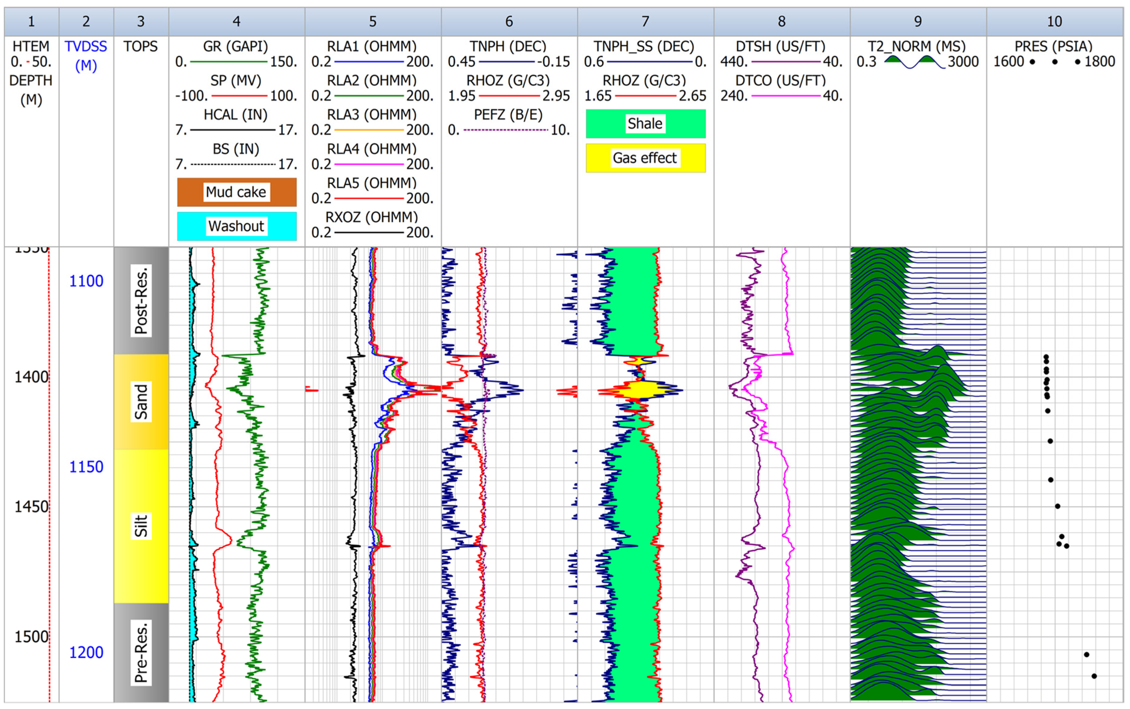
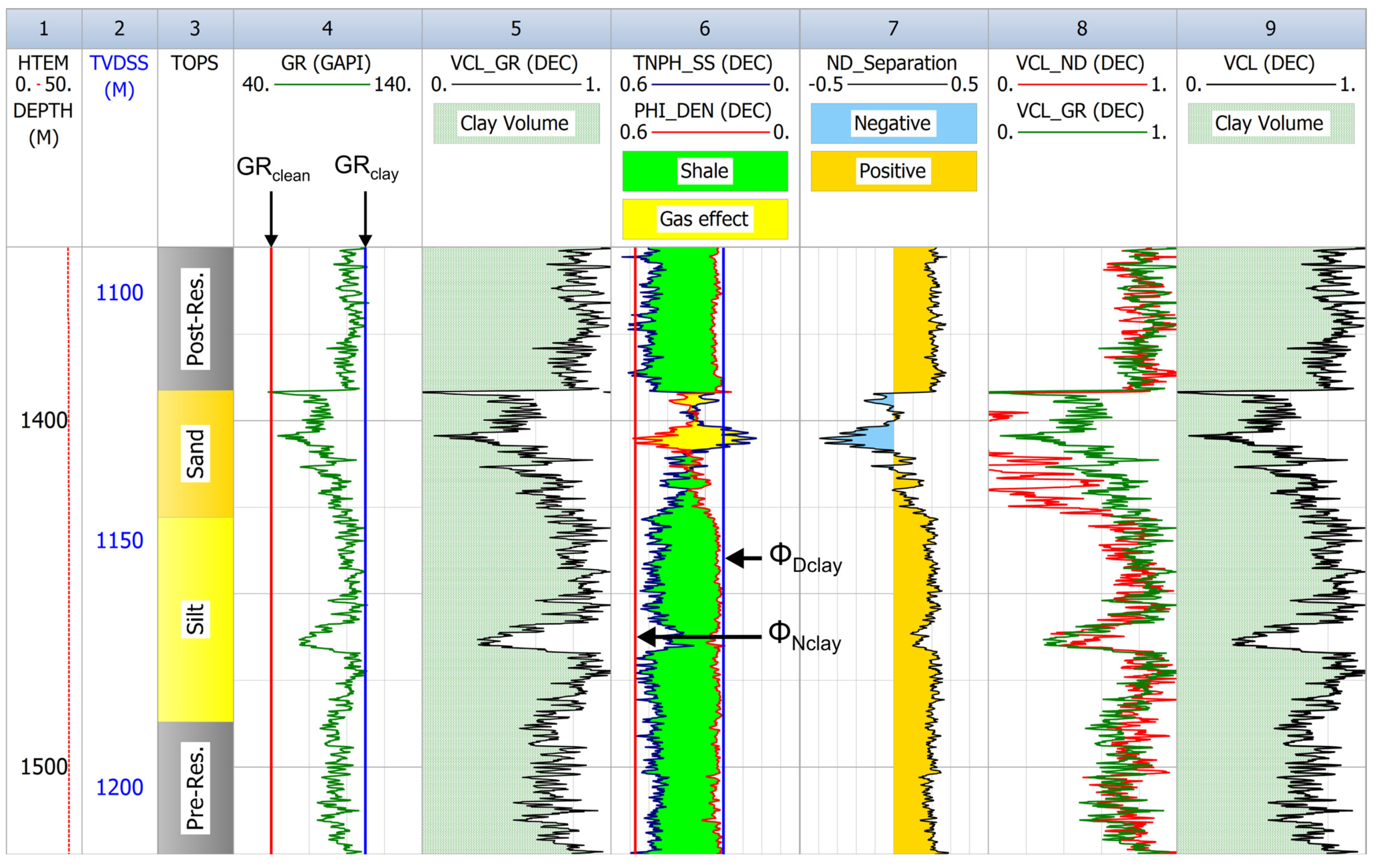
4.1.2. Quantitative Interpretation of Well Logs

A deterministic quantitative interpretation workflow was adopted, based on the combined responses of the density and neutron logs (Figure 5). For this ρ_b = f(ϕ_N) log combination, the hydrocarbon (gas) effects can be accurately corrected and taken into account and ϕ_e is obtained after an iterative and convergent hydrocarbon correction, at each depth level. Unlike sonic logs, neutron and density responses are not affected by the lack of compaction characteristic for young and shallow-depth sands, like the Pliocene reservoirs from “A” and “B” fields.

The “shaly-sands” model used (Figure 6) consists of clean matrix (V_ma) + wet clay (V_clay) + effective porosity (ϕ_e), being defined in terms of fractional volumes as:

$$V_{ma}+V_{clay}+{\varphi }_e=1$$

(10)

$${\varphi }_e={\varphi }_t-V_{CBW}={\varphi }_t-V_{clay}{\varphi }_{clay}$$

(11)

where V_CBW is the volume of clay-bound water and ϕ_clay is the wet clay porosity. A clear distinction is made between the terms “clay” (fraction composed of dry clay minerals and clay-bound water) and “shale” (in the sense of sedimentary rock consisting of a clay fraction and silt-sized particles). The ratio of clay and silt-sized particles in shales is highly variable and one can define a clay:shale ratio (CSR = V_clay/V_shale) or, alternatively, a silt index (I_SILT = V_silt/V_shale). Usually, the clay content in shales may be 40–80%, the silt fraction (V_silt) being treated as part of the clean matrix and having similar properties [31].

The general responses of the density and neutron logs are expressed as:

$${\rho }_b={\rho }_{ma}-V_{clay}\left({\rho }_{ma}-{\rho }_{clay}\right)-{\varphi }_e\left[{\rho }_{ma}-{\rho }_{mf}{S}_{xo}-{\rho }_{hApp}\left(1-S_{xo}\right)\right]$$

(12)

$${\varphi }_N=V_{clay}{\varphi }_{Nclay}+{\varphi }_e\left[{\varphi }_{Nmf}{S}_{xo}+{\varphi }_{NhApp}\left(1-S_{xo}\right)\right]-\Delta {\varphi }_{Nma}-\Delta {\varphi }_{Nex}-\Delta {\varphi }_{Nsal}$$

(13)

where ρ_clay [g/cm³] is the wet clay density, ρ_hApp [g/cm³] is the hydrocarbon (gas) apparent density, ϕ_Nclay [V/V] is the wet clay neutron porosity, ϕ_Nmf [V/V] is the mud filtrate neutron porosity, ϕ_NhApp [V/V] is the hydrocarbon (gas) apparent neutron porosity, Δϕ_Nma [V/V] is the neutron matrix effect (for lithologies other than limestone), Δϕ_Nex [V/V] the neutron excavation effect, Δϕ_Nsal [V/V] is the neutron formation salinity effect, and S_xo [V/V] is the flushed zone water (mud filtrate) saturation. The ϕ_NhApp and ρ_hApp are related to true hydrocarbon density ρ_h [g/cm³] [25,32,33].

The S_xo and S_w water saturations were evaluated in the effective porosity system using the “Indonesia” model [34]:

$$\frac{1}{R_{xo}}=S_{xo}^{n/2}{\left[\frac{V_{clay}^{1-V_{clay}/2}}{\sqrt{R_{clay}}}+\frac{{\varphi }_e^{m/2}}{\sqrt{a R_{mf}}}\right]}^2$$

(14)

$$\frac{1}{R_t}=S_w^{n/2}{\left[\frac{V_{clay}^{1-V_{clay}/2}}{\sqrt{R_{clay}}}+\frac{{\varphi }_e^{m/2}}{\sqrt{a R_w}}\right]}^2$$

(15)

where R_mf [Ω m] and R_w [Ω m] are the mud filtrate resistivity and the formation water resistivity at reservoir temperature and R_clay [Ω m] is the wet clay resistivity. These expressions, which account for the excess conductivity due to clays, are well suited for water saturation evaluation in formations with high clay content and low-salinity formation waters, as expected in the “A” and “B” fields. In Equations (14) and (15), R_xo and R_t were approximated by the MCFL or MLL R_A curves and the deepest-reading Laterolog R_A curves, respectively.

Because ϕ_e and S_xo cannot be determined independently in gas-bearing intervals, an iterative correction is performed using Equations (12)–(14) until ϕ_e and S_xo convergence, then S_w is derived from Equation (15) and the converged ϕ_e solution.

To provide an independent and continuous V_clay estimation as input in Equations (12) and (13), GR logs were used as main clay indicators. Several studies [31,35,36] have shown that the GR response in shaly formations should increase linearly with the clay volume fraction. The linear V_clayGR [V/V] clay volume estimator is defined via a gamma-ray index I_GR [V/V] [22,27,37]:

$$V_{clayGR}=I_{GR}=\frac{GR-G{R}_{clean}}{G{R}_{clay}-G{R}_{clean}}$$

(16)

where GR_clean [gAPI] is the gamma-ray background radioactivity of clean reservoir rocks and GR_clay [gAPI] is the gamma-ray radioactivity of clays. To verify that the relatively low-contrast GR logs recorded in the analyzed wells can be used as valid clay volume estimators, V_clayGR were checked against independently derived neutron–density V_clayND [V/V] estimations:

$$V_{clayND}=\frac{{\varphi }_N-{\varphi }_D}{{\varphi }_{Nclay}-{\varphi }_{Dclay}}$$

(17)

$${\varphi }_{Dclay}=\frac{{\rho }_{ma}-{\rho }_{clay}}{{\rho }_{ma}-{\rho }_{mf}}$$

(18)

where ϕ_N is the matrix-corrected neutron apparent porosity (referenced to sandstone lithology), ϕ_D is given by Equation (5), and ϕ_Dclay [V/V] is the wet clay density porosity. The neutron–density combination is one of the best clay indicators in good hole conditions and water-bearing intervals but is affected by washouts or rugose zones and computes negative V_clayND values in gas-bearing intervals where distinctive crossovers (ϕ_N < ϕ_D) occur. The clay indicators comparison allowed the tuning of the GR_clean and GR_clay endpoints, using as a reference (V_clay = 1) the maximum and repeatable separations ϕ_Nclay − ϕ_Dclay, to obtain V_clayGR ≈ V_clayND over the largest part of the intervals. For the analyzed wells, the GR_clean range was 45–60 gAPI, the GR_clay range was 100–114 gAPI, and the reference ϕ_Nclay − ϕ_Dclay maximum separation range was 0.23–0.29. Figure 7 shows an example of the V_clay indicators comparison for the A-2 well, over an interval that includes the post-reservoir, reservoir, and pre-reservoir sections. No nonlinearity was observed on V_clayGR = f(V_clayND) crossplots for any of the wells, thus validating the adopted linear V_clayGR estimator.

The wet clay parameters (ρ_clay, ϕ_Nclay, R_clay) were statistically derived from ρ_b, ϕ_N, and R_t histograms and GR = f(ρ_b), GR = f(ϕ_N), and GR = f(R_t) frequency crossplots, as the most repeatable readings in the shaliest intervals delineated through a GR > GR_cut-off criterion. The mean ρ_ma, m, and n values measured on cores at quasi-reservoir overburden pressure were used for all the wells, along with the R_w values estimated in the pre-interpretation phase and confirmed or slightly refined during the interpretation. Gas density (ρ_h) was estimated considering the true vertical depths (TVDs) of the reservoirs, the hydrostatic pressures, and the measured temperatures.

Table 4. Main log-derived and core-derived parameters used for the effective porosity (ϕ_e) and water saturations (S_xo, S_w) evaluation in the reservoir intervals of “A” and “B” fields.

Well	ρma [g/cm3]	ρmf [g/cm3]	ρh [g/cm3]	ρclay [g/cm3]	ϕNclay [V/V]	a	m	n	Rclay [Ω m]	Rw [Ω m]	Rmf @ Tmf [Ω m @ °C]
A-1	2.68	1.050	0.082	2.26	0.46	1	1.71	1.67	6.00	0.600	0.123 @ 12
A-2	2.68	1.020	0.082	2.25	0.49	1	1.71	1.67	7.90	0.600	0.185 @ 25
B-1	2.71	1.060	0.080	2.26	0.50	1	1.54	1.32	8.50	1.100	0.081 @ 18
B-2	2.72	1.049	0.085	2.26	0.50	1	1.54	1.32	7.50	1.040	0.115 @ 17
B-3	2.71	1.036	0.084	2.26	0.45	1	1.54	1.32	5.20	0.950	0.116 @ 25
B-4	2.71	1.026	0.082	2.25	0.48	1	1.54	1.32	7.80	1.175	0.137 @ 28

R_mf @ T_mf—Mud filtrate resistivity at surface measurement temperature.

synthesizes the main log-derived and core-derived interpretation parameters.

4.2. Wireline Formation Pressure Data Processing and Analysis

In favorable conditions, wireline formation pressure data allow the identification of the reservoir fluid contacts (gas–water contact—GWC, oil–water contact—OWC and gas–oil contact—GOC), the classification of fluid types (in situ densities), and, also, the assessment of fluids separation via permeability barriers.

The depths of the fluid contacts are critical for calculating the volume of hydrocarbons in the reservoirs and important for increasing the accuracy of well log interpretations, such as porosity evaluation in the case of reservoirs with multiple fluids and different physical properties. The available methods for locating the fluid contacts include fluid sampling (from drill stem tests or wireline formation testers), analysis of log-derived or core-derived fluid saturations variation with depth, and pressure profile surveys.

The normal (hydrostatic) pore pressure p measured at a particular depth z = TVDSS (true vertical depth subsea) is given by:

$$p={\rho }_f g z$$

(19)

where ρ_f is the fluid density and g is the acceleration of gravity (≈9.81 m/s²). If the pressures p₁ and p₂ are measured at different depths z₁ and z₂,

$$p_2-p_1={\rho }_f g \left(z_2-z_1\right)\to \Delta p={\rho }_f g \Delta z \to \frac{\Delta p}{\Delta z}={\rho }_f g$$

(20)

one can define a pressure–depth gradient (trend) Δp/Δz, where Δp = p₂ − p₁ and Δz = z₂ − z₁. If a single fluid is present in the pore space of the formations, successive pressure measurements carried out at various depths will define a single pressure–depth gradient. For multiple fluids with significantly different densities, a p = f(z) plot will show changes in the slope corresponding to multiple pressure–depth gradients, e.g., (Δp/Δz)₁ and (Δp/Δz)₂. The depths where the pressure trends are changing define the position of the fluid contacts (Figure 8) and the density of the reservoir fluids can be inferred from the gradients (e.g., ρ_f1 = (Δp/Δz)₁/g and ρ_f2 = (Δp/Δz)₂/g).

Regression analysis was performed using the wireline pressure datasets of the wells from “A” and “B” fields, for deriving meaningful pressure–depth trends related to reservoir fluids type and their in situ densities. The trends were subsequently used to locate the likely GWCs, which were compared with the results of quantitative well log interpretation and of NMR data processing.

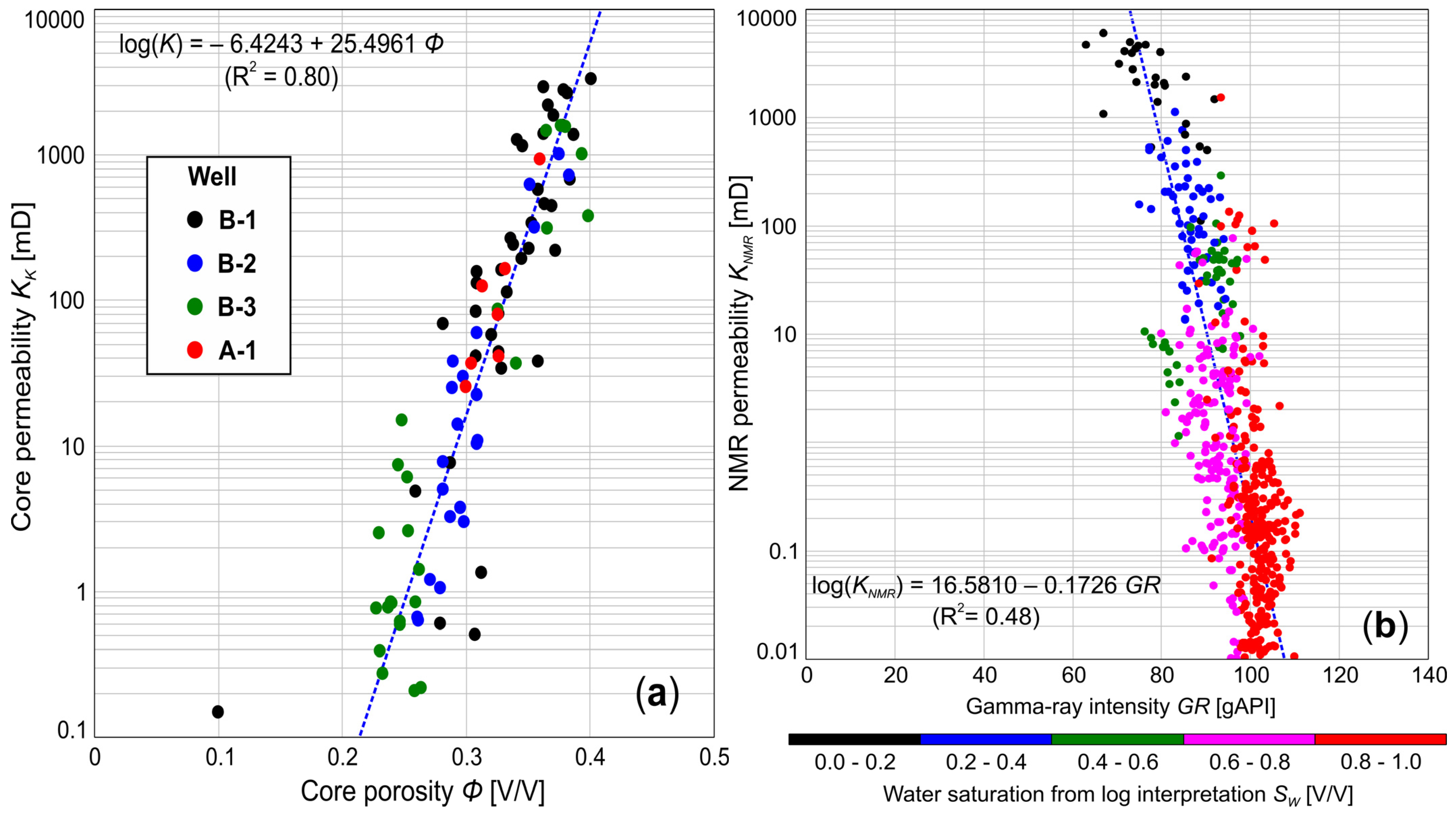
4.3. Permeability Modeling

The analysis of core data from “A” and “B” fields shows a strong correlation between K_k and ϕ (Figure 9a), indicating that porosity is the main factor controlling the formations permeability. The inverse correlation between permeability and shaliness (i.e., permeability decreases with increasing clay content) is illustrated via well logging data by the K_NMR = f(GR) dependency from Figure 9b, which also shows the inverse correlation between K_NMR and S_w.

For all the wells from “A” and “B” fields, continuous permeability curves were modeled via a multiple linear regression (MLR) technique, by fitting in the least-squares sense exponential functions of the type K = f(ϕ_e, V_clay) or K = f(ϕ_e, V_clay, S_w). The predicted permeability curves that were tested had the form:

$$K={10}^{\left(a+b {\varphi }_e+c V_{clay}\right)}$$

(21)

$$K={10}^{\left(a+b {\varphi }_e+c V_{clay}+d S_w\right)}$$

(22)

where a, b, c, and d are computed polynomial regression coefficients that allow the best possible reconstruction of the input control (reference) permeability datasets.

The control data for the best fit of permeability functions was provided by: (a) the sets of depth-shifted and log-matched permeability measurements on core plugs available for the A-1, B-1, B-2, and B-3 wells; (b) the NMR-derived formation permeability estimated for the A-2 well. The permeability modeling was carried out both for each well and also at the field level, by jointly fitting synthetic K curves to the multiple discrete-continuous (core- and NMR-derived) or solely discrete (core-derived) control datasets from fields “A” and “B”, respectively.

5. Results and Discussion

The Early Pliocene gas-bearing reservoirs from the “A” and “B” fields (Figure 3 and Figure 4) appear on well logging data with a characteristic signature, i.e., a coarsening upward and suppressed gamma-ray configuration (limited contrast between the reservoir and non-reservoir intervals), few intervals with neutron-density gas crossover as a consequence of clay content, and locally suppressed resistivity response but with a clear increased sonic Δt_c response (low P-wave velocity). There is a large discrepancy between the maximum recorded deep R_A resistivities in the “Sand” main reservoir unit from the two fields: A-1 well—170 Ω m, A-2 well—371 Ω m, B-1 well—16 Ω m, B-2 well—17 Ω m, B-3 well—26 Ω m, B-4 well—82 Ω m. The likely underestimated R_A readings may be explained by an averaging effect upon the Laterolog tools, when investigating thin beds with a thickness less than the vertical resolution (a core extracted from the “Sand” unit in well B-3 shows sand/silt laminations with thicknesses ranging from few mm to 10–15 cm, interbedded with muds). This limitation could be mitigated in future studies by investigating the ability of advanced resistivity logging tools, such as the Rt Scanner service (Schlumberger Ltd.), to resolve the thinly laminated reservoir sand beds and provide more realistic resistivity readings for accurate water and gas saturations determination.

The main results of the wireline logging data processing for the analyzed wells are presented and discussed in the following sections.

5.1. Formation Waters

Figure 10a,b show examples of Hingle-type crossplots corresponding to B-2 and B-4 wells, constructed in the pre-interpretation phase and including the “Sand”, “Silt”, and short post-reservoir Pliocene intervals comprising clean sand beds. Data points are color-coded according to the GR intensity. The input porosity ϕ = ϕ_D was computed for a matrix density ρ_ma = 2.71–2.72 g/cm³ (mean of core-derived measurements) and a pore fluid density ρ_mf ≈ 1.04 g/cm³; the Archie parameters used were derived from SCAL measurements (m = 1.54, n = 1.32). Rt was approximated by the deep investigation Laterolog R_A curves (LLD and RLA5). The datasets were filtered via gamma-ray and caliper cut-offs (GR < 70 gAPI, d < 9 in), to retain reasonably clean levels with good hole conditions. Forced least-squares regressions through the matrix point (ϕ = 0, R_t → ∞) and the linear trend of NW located data points identified the water-bearing levels (S_w = 1 “water line”) and yielded from the maximum slope 1/R_w^(1/m): R_w = 1.04 Ω m (equivalent salinity: 3932 ppm NaCl) for B-2 well and R_w = 1.175 Ω m (equivalent salinity: 3475 ppm NaCl) for B-4 well. The data points that define the linear water-bearing trends belong not only to clean sand beds in the post-reservoir sections, but also to few levels within the “Sand” and “Silt” units. This indicates that the main reservoirs and the post-reservoir Pliocene deposits in their proximity likely host similar or identical formation water in the pore space. Consequently, the R_w values obtained from the resistivity–porosity analyses are suitable for the quantitative evaluation of the main reservoirs in terms of fluid saturations.

Figure 11a presents an example of Pickett-type crossplot for B-3 well, including data from the “Sand”, “Silt”, and post-reservoir intervals (caliper cut-off applied to the data: d < 9 in). The final ϕ_e resulting from log interpretation was used and Rt was approximated by the RLA5 deep Laterolog curve. Figure 11b shows the same crossplot with a GR < 70 gAPI cut-off applied, to retain only the relatively clean levels. A robust least-squares regression through the linear trend of the lowermost data clearly defined the S_w = 1 line, confirmed the SCAL-derived cementation exponent from the slope (−1/m) of the best-fit line, and provided R_w = 0.95 Ω m (equivalent salinity: 4320 ppm NaCl). The data points defining the linear aquifer trend correspond to clean sand beds from the post-reservoir section and also to some levels from the “Sand” and “Silt” reservoirs, suggesting again that the formation waters have a constant resistivity and salinity throughout the analyzed sequence.

In Figure 11a, it can be noticed that the location of the S_w = 1 line coincides with the onset of the log(ϕ) = f(log(R_t)) change of trend, from a quasi-vertical data distribution in claystones and mudstones/shales towards a slight R_t increase in the gas-bearing reservoir. In the specific petrophysical context of fields “A” and “B”, this feature has a methodological importance if such crossplots are used over intervals with very limited porosity and resistivity variation range, when it is difficult to identify a clear linear trend of the water-bearing data.

A comparable result was obtained for B-1 well using the same approach: R_w = 1.10 Ω m at formation temperature (equivalent salinity: 3719 ppm NaCl). One may observe that the formation water resistivities and salinities obtained for the wells of field “B” are almost identical, regardless of: (a) the different porosity and resistivity ranges that defined the water-bearing trend (Figure 10) and (b) the input porosity type or the type of resistivity–porosity crossplot.

Figure 12a,b show Pickett-type crossplots for A-1 and A-2 wells, including data from the “Sand”, “Silt”, and post-reservoir intervals (caliper cut-off applied to the data: d < 9 in). The crossplots were constructed using the final ϕ_e from log interpretation, Rt approximated by the RLA5 deep Laterolog R_A curve, and Archie parameters obtained from the SCAL measurements. An S_w = 1 linear regression with a fixed slope (m = 1.71) fitted through the start of the data distribution change of trend provided R_w = 0.6 Ω m for both wells (equivalent salinity: 7000 ppm NaCl).

The presented R_w results, determined over slightly larger depth intervals than the main reservoir units of the “A” and “B” fields, may be considered as representative for the Pliocene deposits including the reservoirs. These R_w values were used for S_w evaluation for all the analyzed wells.

5.2. Petrophysical Interpretation

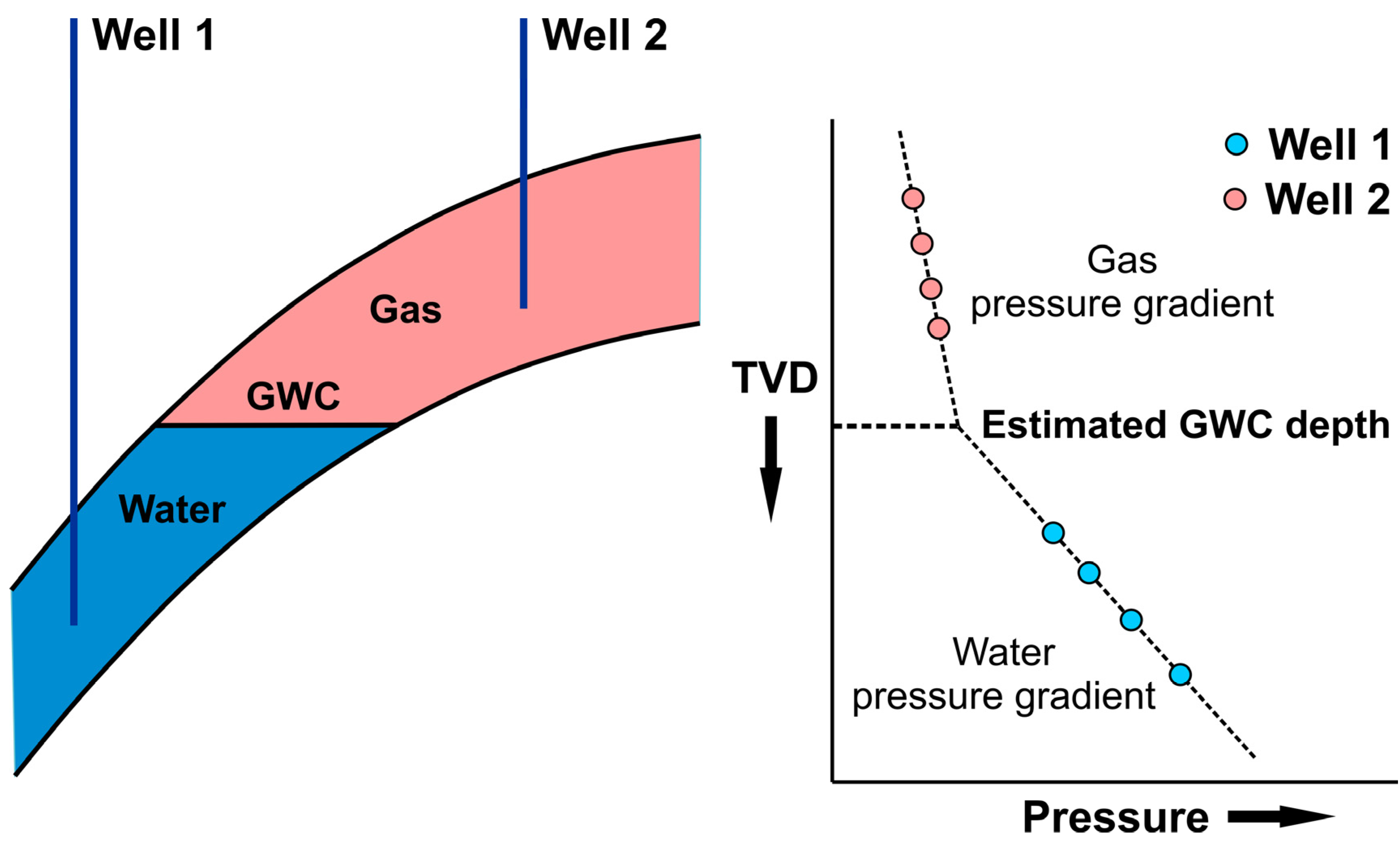
Figure 13, Figure 14 and Figure 15 illustrate examples of deterministic quantitative interpretation results for the wireline logging data recorded in the final sections of A-1, A-2, and B-2 wells. The main interpretation parameters were presented in Table 4, with ρ_ma, m, and n obtained from measurements on core plugs at quasi-reservoir overburden pressure.

The final petrophysical solutions are presented in Figure 13—tracks 7–9, Figure 14—tracks 6–8, and Figure 15—tracks 7–9: computed S_w and S_xo water saturations, bulk volumes of formation fluids (water in the uninvaded zone ϕ_eS_w, water in the flushed zone ϕ_eS_xo, movable hydrocarbons ϕ_e(S_xo − S_w), residual hydrocarbons ϕ_e(1 − S_xo), and the lithological fractions (V_clay, V_silt, V_ma, ϕ_e). Tracks 9–10 from Figure 14 show the raw NMR data (normalized T₂ transverse relaxation time distribution) and the NMR interpretation results in terms of clay-bound water (CBW), capillary-bound water (BVI), and free fluid (FFI) volumes, as well as the NMR-derived permeability (NMR_K).

Two distinct gas-bearing reservoir intervals separated by permeability barriers were identified in the conventional “Sand” and “Silt” units from both fields (R1 and R2 in Figure 13, Figure 14 and Figure 15), the reservoirs’ separation being more evident in field “A”. The upper reservoir located in the “Sand” unit is better developed, with a 29 m thickness in well A-1 and 24.5 m in well A-2, and characterized by higher overall porosities (well A-1: maximum ϕ_e = 37%, mean ϕ_e = 21.6%; well A-2: maximum ϕ_e = 32%, mean ϕ_e = 15.7%). The thickness of the secondary reservoir ranges from 17 m in well A-1 to 6 m in well A-2, the porosities being lower (well A-1: maximum ϕ_e = 26%, mean ϕ_e = 14.0%; well A-2: maximum ϕ_e = 24%, mean ϕ_e = 14.8%). In well B-2 (field “B”), the gas-bearing reservoirs delineated within the “Sand” and “Silt” conventional units are comparable, with a 12.5–13 m thickness, mean ϕ_e of 14.4–15.2%, and maximum ϕ_e of 27–36%.

The minimum water saturations (maximum gas saturations) computed in the reservoir intervals from the “Sand” units were: A-1 well—S_w,min = 8.2% (S_h,max = 91.8%), A-2 well—S_w,min = 4.4% (S_h,max = 95.6%), B-1 well—S_w,min = 34.8% (S_h,max = 65.2%), B-2 well—S_w,min = 33.8% (S_h,max = 66.2%), B-3 well—S_w,min = 34.9% (S_h,max = 65.1%), B-4 well—S_w,min = 9.1% (S_h,max = 90.9%). Rapid alternations of resistive (gas-bearing sands) and conductive (claystones or mudstones/shales) thin beds or laminations, as the ones observed in cores extracted from the field “B” wells, may not be correctly resolved by the Laterolog tools used. Due to this resistivity suppression (the maximum R_A readings in the gas-bearing intervals of field “B” field are one order of magnitude lower than those recorded in the wells from field “A”), the S_w,min values computed for B-1, B-2, and B-3 wells may be overestimated and the S_h saturations underestimated.

The NMR log interpretation results revealed additional sources of resistivity suppression and possible S_h underestimation even in clean, thick reservoirs. In the wells A-2, B-2, B-3, and B-4, the deep R_A maximum readings and the corresponding S_w,min and S_h,max computed saturations do not occur at the tops of the gas-bearing intervals but below them (e.g., the top of R1 reservoir—tracks 5 and 6 in Figure 14). This is caused by a large amount of irreducible capillary-bound water trapped in small pores and hosted at the top of the reservoir intervals (note the 13% capillary-bound water volume at 1125 m TVDSS, in Figure 14—track 10). The presence of silt layers on top of underlying sands, possibly due to underwater sediment gravity flows followed by graded bedding, could explain such abnormal low-resistivity zones, which, however, may produce water-free gas.

The validity of the quantitative log interpretations was evaluated by: (a) comparison between log-derived petrophysical parameters and the same parameters resulted from RCAL and SCAL core measurements at quasi-reservoir overburden pressure; (b) reconstruction of the theoretical response of water-saturated formations by means of a “wet resistivity” curve R₀ = F R_w = a ϕ_e^−m R_w and its comparison with the recorded deep investigation Laterolog R_A curves. An example of the comparison and good agreement between log-derived S_w and ϕ_e and the core-derived equivalents (CORE_SW—water saturation measured on core plugs at 1200 psig pressure, CORE_PHI—porosity measured on core plugs at 1400 psig pressure) is shown in Figure 13—tracks 11 and 12. The resistivity comparison control criterion is illustrated in Figure 13—track 6, Figure 14—track 5, and Figure 15—track 6. The close match between the measured deep resistivities (RLA5, RLLD) and the theoretical R₀ curves, except in gas-bearing intervals, indicates that the log-derived (R_w, ρ_clay, ϕ_Nclay) and core-derived (ρ_ma, m, n) interpretation parameters were adequate, and the saturation model used was realistic—Equations (14) and (15).

At the scale of the analyzed reservoirs, the MLR technique was found to be effective in predicting continuous permeability curves, with control provided by any available set of permeability measurements. Track 13 from Figure 13 illustrates the fit of a function K = f(ϕ_e, V_clay, S_w) simultaneously for A-1 and A-2 wells, by jointly using multiple control datasets: the Klinkenberg-corrected permeabilities (CORE_K) measured on core plugs from well A-1 at 1400 psig overburden pressure and the continuous K_NMR curve from A-2 well (NMR_K in Figure 14—track 10). The modeled permeability curve MLR_K [mD] = 10^(8.730999 − 11.858403 ϕ_e − 6.703942 V_clay − 5.804627 S_w) is shown in track 12. Another example is presented in Figure 15—track 10, where a synthetic permeability curve MLR_K [mD] = 10^(0.44883338 + 9.57922687 ϕ_e + 0.18209513 V_clay − 3.25371721 S_w) provided a close fit to the set of Klinkenberg-corrected permeabilities (CORE_K) measured on core plugs from well B-2 at quasi-reservoir pressure.

It is noticeable that slight background gas saturations resulted from the log interpretation in the pre-reservoir (Late Miocene/Pontian, generally argillaceous deposits) sections of the analyzed wells (e.g., Figure 14 and Figure 15), confirming gas shows reported while drilling. Taking into account the widespread methane seepage phenomena in the younger sediments of the Black Sea offshore area, we consider these minor gas saturations as petrophysical evidences of an active/ongoing gas migration process from the deeper levels of the Miocene pelitic deposits.

5.3. Fluid Contacts

Figure 16 and Figure 17 show the wireline formation pressure datasets from fields “A” and “B” (three outlying pressure readings from well B-1 at TVDSS 1784.4, 1787.4, and 2461.9 m were removed). For both fields, the depth coverage with pressure readings (including pre-reservoir Pontian deposits and post-reservoir Dacian–Romanian deposits) allowed an adequate definition of the formation water trend. The contrasting gas trend was better outlined in field “A” than in field “B”, due to the larger amount of data and higher gas saturations. At a field-level scale, the intersection of the hydrostatic pressure trends corresponding to the two reservoir fluids suggest GWC depths of 1157.5 m TVDSS for field “A” and 1123.1 m TVDSS for field “B” (for relatively permeable and gas-bearing reservoirs, the GWC depths normally correspond to the free water levels—FWLs). The pressure–depth gradients computed for field “A” were (Δp/Δz)₁ = 0.396 psia/ft (0.089 bar/m) and (Δp/Δz)₂ = 0.071 psia/ft (0.016 bar/m), corresponding to in situ fluid densities ρ_f1 = 0.913 g/cm³ (water) and ρ_f2 = 0.163 g/cm³ (gas). For field “B”, the computed gradients were (Δp/Δz)₁ = 0.439 psia/ft (0.099 bar/m) and (Δp/Δz)₂ = 0.116 psia/ft (0.026 bar/m), corresponding to fluid densities ρ_f1 = 1.013 g/cm³ (water) and ρ_f2 = 0.267 g/cm³ (gas). Except the water density obtained for field “B” (aquifer trend defined by p [psia] = 1.441 TVDSS [m] + 24.267), the other inferred fluid densities are either too low or too high with respect to the likely ρ_w (≥ 1 g/cm³) and to the ρ_h predicted by the ideal gas law (≈ 0.08 g/cm³). The inaccuracy of reservoir fluid densities estimation implies the uncertainty of GWC depths estimation from wireline pressure data.

The results of a detailed pressure data analysis performed for each well of the “A” and “B” fields are synthesized in

Table 5. Results of wireline formation pressure data processing and interpretation: pressure–depth gradients, fluid densities, and GWC depths estimated from the gradients’ slope and intersection.

Well	Fluid 1 (Water) Pressure Trend [psia] [m TVDSS]	Fluid 1 (Water) Density [g/cm3]	Fluid 2 (Gas) Pressure Trend [psia] [m TVDSS]	Fluid 2 (Gas) Density [g/cm3]	GWC Estimated Depth [m TVDSS]
A-1	Pressure = Depth ∙ 1.372 + 106.353	0.964	Pressure = Depth ∙ 0.197 + 1465.902	0.139	1157.7
A-2	Pressure = Depth ∙ 1.227 + 275.749	0.863	Pressure = Depth ∙ 0.304 + 1344.683	0.214	1158.4
B-1	Pressure = Depth ∙ 1.442 + 30.645	1.014	N/A	N/A	N/A
B-2	Pressure = Depth ∙ 1.444 + 18.131	1.015	Pressure = Depth ∙ 0.090 + 1540.003	0.064	1124.4
B-3	Pressure = Depth ∙ 1.453 + 2.950	1.022	N/A	N/A	N/A
B-4	Pressure = Depth ∙ 1.451 + 0.798	1.020	Pressure = Depth ∙ 0.230 + 1380.782	0.162	1130.3

.

For wells B-1 and B-3, the insufficient data coverage in the “Sand” and “Silt” reservoir units allowed the delineation of a single pressure trend related to formation water. For the wells of field “A”, the estimated density of “fluid 1” (water) was lower than the anticipated ρ_w and the estimated density of “fluid 2” (gas) was significantly higher than the likely gas density ρ_h. For the wells of field “B”, the estimated ρ_w was veridical but ρ_h was lower or higher than expected. This uncertainty can be partially explained by the small number of pressure measurements in the reservoir intervals of field “B”. However, for field “A”, the deviations of estimated ρ_w and ρ_h from the expected values cannot be explained by insufficient pressure data.

The quantitative well log interpretation proved extremely useful for evaluating the validity of GWC estimations based on pressure data. The formation pressure measurements and the pressure–depth trends for the wells A-1, A-2, and B-2 are displayed in Figure 13—track 10, Figure 14—track 11, and Figure 15—track 11 (the horizontal dashed line marks the pressure trends intersection, i.e., the GWC estimated from pressure data). The petrophysical analysis results indicate that distinct fluid contacts should be considered within each of the reservoirs, instead of a single “averaging” GWC obtained exclusively from a pressure survey. The log-based fluid contact depths (GWC1, GWC2) were delineated at the base of the gas column in each reservoir, where a significant decrease in the computed S_w values occurs. As observed, there are significant depth differences between the two types of estimations, ranging from 4.1 to 15.4 m. Besides the questionable fluid densities, an additional indication regarding the uncertainty of pressure-based fluid contact depths was provided by the NMR log available for well A-2 (Figure 14—tracks 9, 10). The GWC estimated from the formation water and gas pressure trends at 1158.4 m TVDSS is located in an impermeable mudstone/shale interval that separates the two gas-bearing reservoirs. At that depth, the NMR results show no free fluids but only bound (immobile) water.

Especially for field “A”, the ρ_w underestimation and ρ_h overestimation may be explained by considering that the wireline testers did not read pressures corresponding to true formation water and gas, but to mixtures of water (mud filtrate) and gas or gas and water, respectively. Additionally, the small number of pressure readings outside the “Sand” and “Silt” units, in the pre-reservoir and post-reservoir intervals of field “A”, did not allow a better definition of the water trend. The more realistic ρ_w values estimated for field “B” and the GWC depth obtained for well B-2 (1124.4 m TVDSS), closer to the log-based fluid contacts, could be attributed to actually lower gas saturations in the “Sand” and “Silt” units of that field.

6. Conclusions

This study aimed to present and discuss the main issues related to the petrophysical evaluation of two biogenic dry gas fields of Early Pliocene (Dacian) age from the Romanian continental shelf—Western Black Sea basin (conventionally denoted “A” and “B”). The sands and silts reservoirs have a better quality in field “A”, developed in a shallow marine environment, than in the marginal marine (deltaic) field “B”, which shows a higher silt content, fewer thick sand intervals, and frequent thinly laminated sand-shale sequences. A vertical, coarsening upward, variability of the reservoirs generally exists in both fields, with silty deposits in the lower part of the reservoir intervals overlain by sands.

The quantitative interpretation of the wireline well logs recorded in six exploration wells was performed using a deterministic workflow. Some of the interpretation parameters (ρ_ma, m, and n) were derived from routine and special analyses carried out on core plugs at quasi-reservoir confining pressure, whereas the other parameters (ρ_clay, ϕ_Nclay, R_clay, R_w) were estimated statistically or via crossplot techniques from the logs. The formation pressure data measured in all the wells were processed and interpreted in terms of probable gas–water contact (GWC) depths, which were evaluated by comparison with the results of well log interpretation.

A significant problem that affected the well log interpretation in the analyzed fields was the uncertainty related to R_w values and, consequently, to S_w and S_h evaluation. Without representative water samples collected (uncontaminated by drilling mud filtrate) no accurate and direct R_w information was available. On the other hand, no obvious water-bearing beds were discernible within the Dacian reservoir intervals. The approach used in this study for obtaining realistic R_w values was the analysis of resistivity–porosity dependencies over slightly extended depth intervals, which included the Dacian reservoirs and short sections of post-reservoir Pliocene deposits where clean and probably water-bearing sand beds were present.

The main conclusions emerging from this study are:

• The integration of core measurements in the well log interpretation methodology had a major impact on the validity of the obtained results. Core-derived petrophysical measurements were used both as input computation parameters and also to check and validate the main reservoir parameters resulted from the interpretation (ϕ, S_w, K). Additionally, the core-derived ρ_ma and m provided the necessary constraints for the realistic estimation of R_w from resistivity–porosity dependencies;
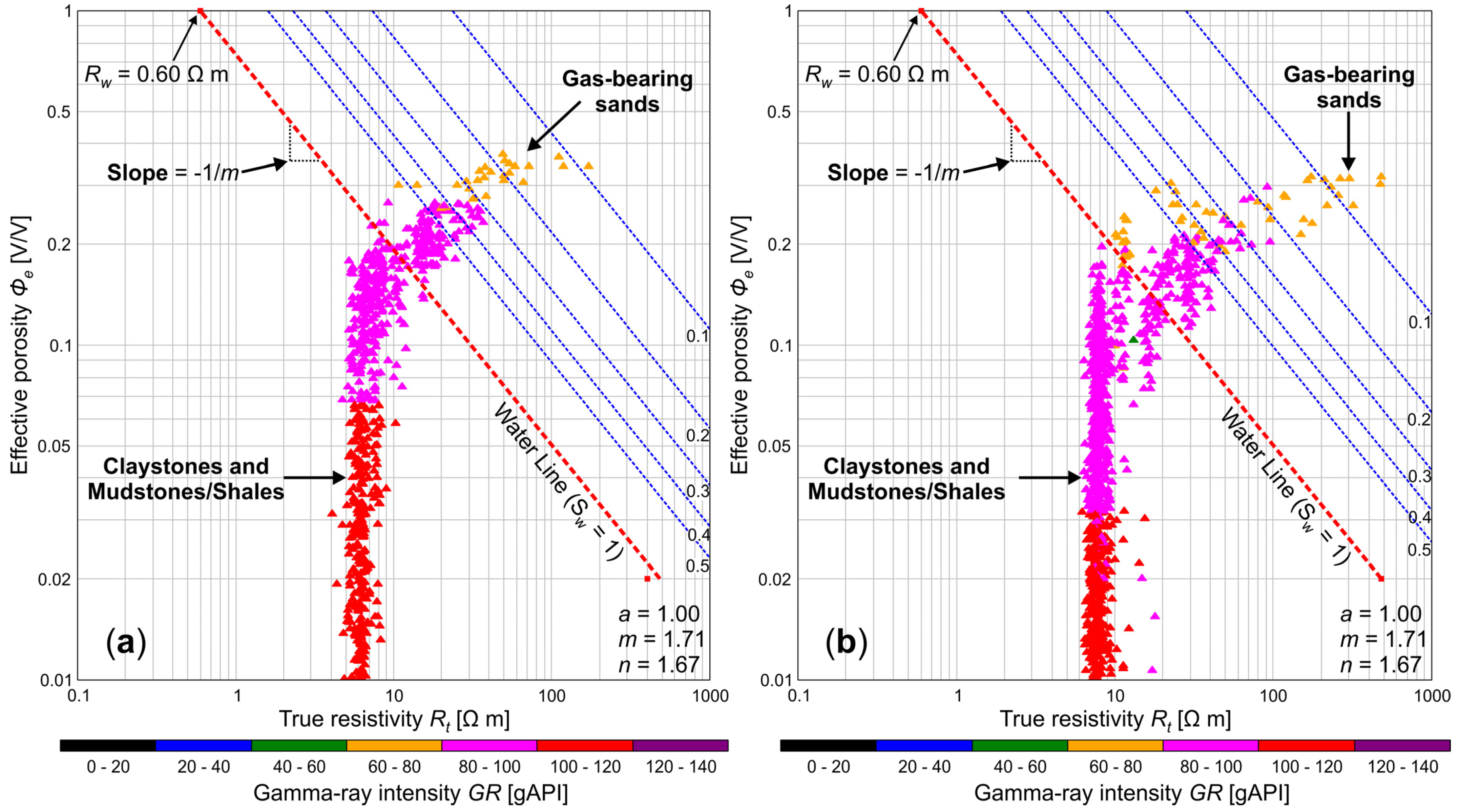
• The approach used for R_w estimation, i.e., the use of resistivity–porosity dependencies and the extension of the analysis interval to segments of Pliocene deposits above the gas-bearing reservoirs, proved to be effective. The capability of R_t–ϕ dependencies to reveal linear data trends in clean water-bearing formations with constant R_w showed that parts of the Dacian reservoirs (the very limited bottom water zones underneath the gas columns) and the adjacent post-reservoir Pliocene sections host similar formation waters. This allowed the determination of realistic R_w values, which were used for S_w evaluation in the analyzed wells;
• Particularly in the “B” field, the Laterolog (DLL and HALS) resistivity curves are likely suppressed to varying degrees in each well, leading to possible S_w overestimation and S_h underestimation and negatively impacting gas reserve evaluation. One cause of this problem may be represented by the alternance of thin (millimeter to decimeter thick) resistive and conductive layers of sand and mudstone/shale, which are averaged by the resistivity tools due to their limited vertical resolution;
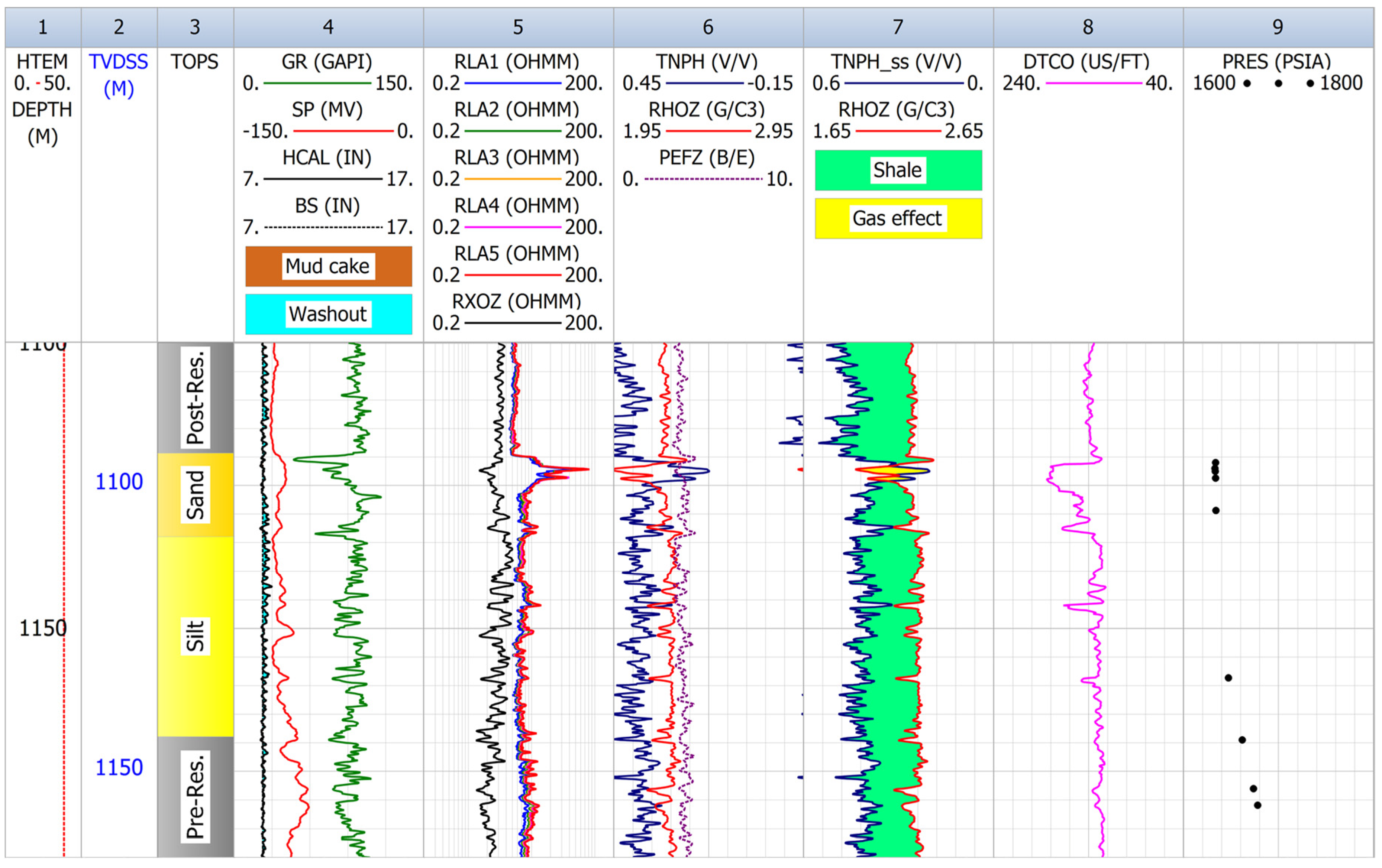
• An additional source of resistivity logs suppression, both in “A” and in “B” fields, is represented by a high content of capillary-bound water, probably trapped in the small pores of silt intervals. The NMR logging performed in well A-2 from field “A” was essential for understanding the cause of these low-resistivity intervals, sometimes located at the top of resistive gas-bearing reservoirs sands;
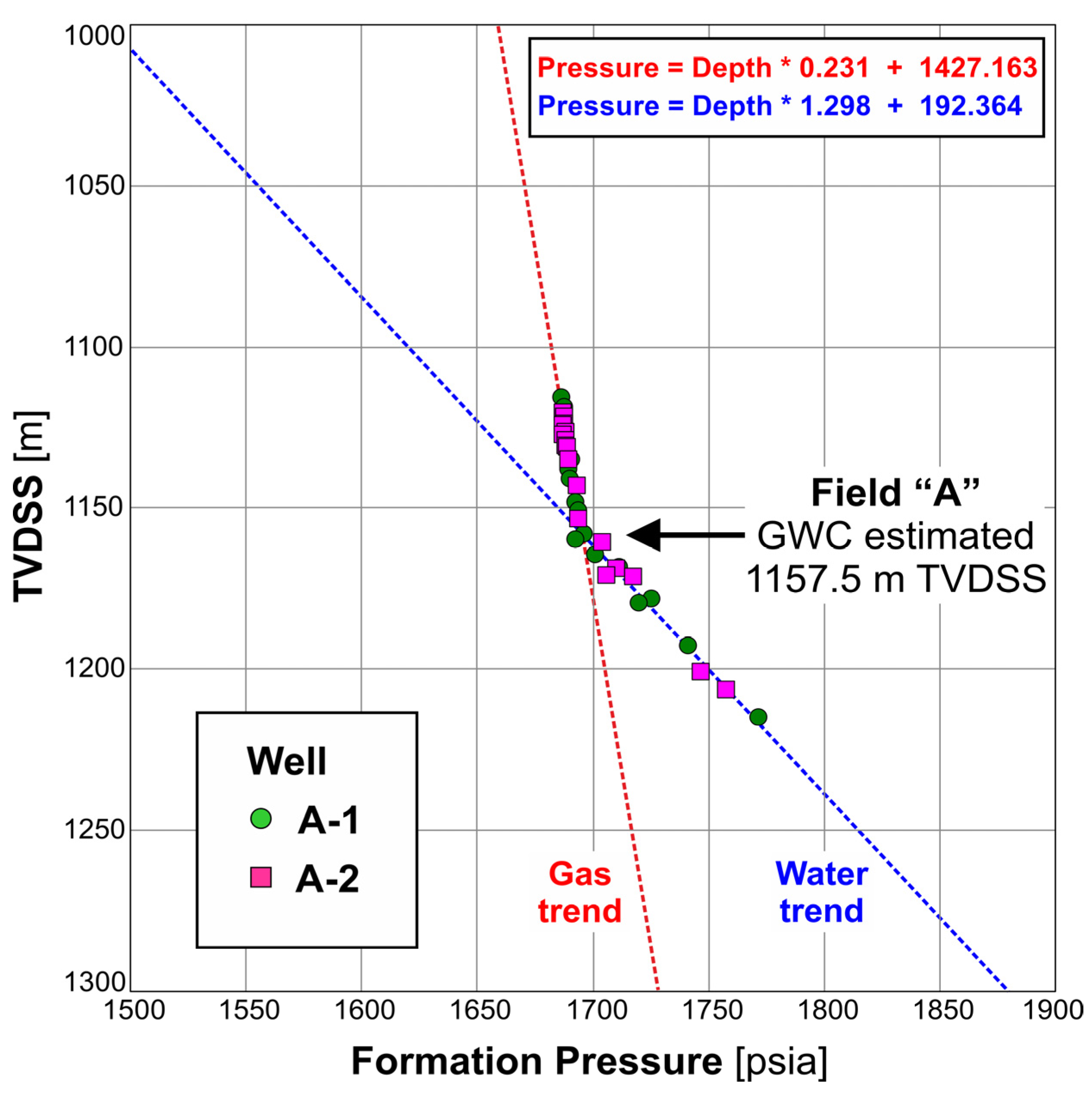
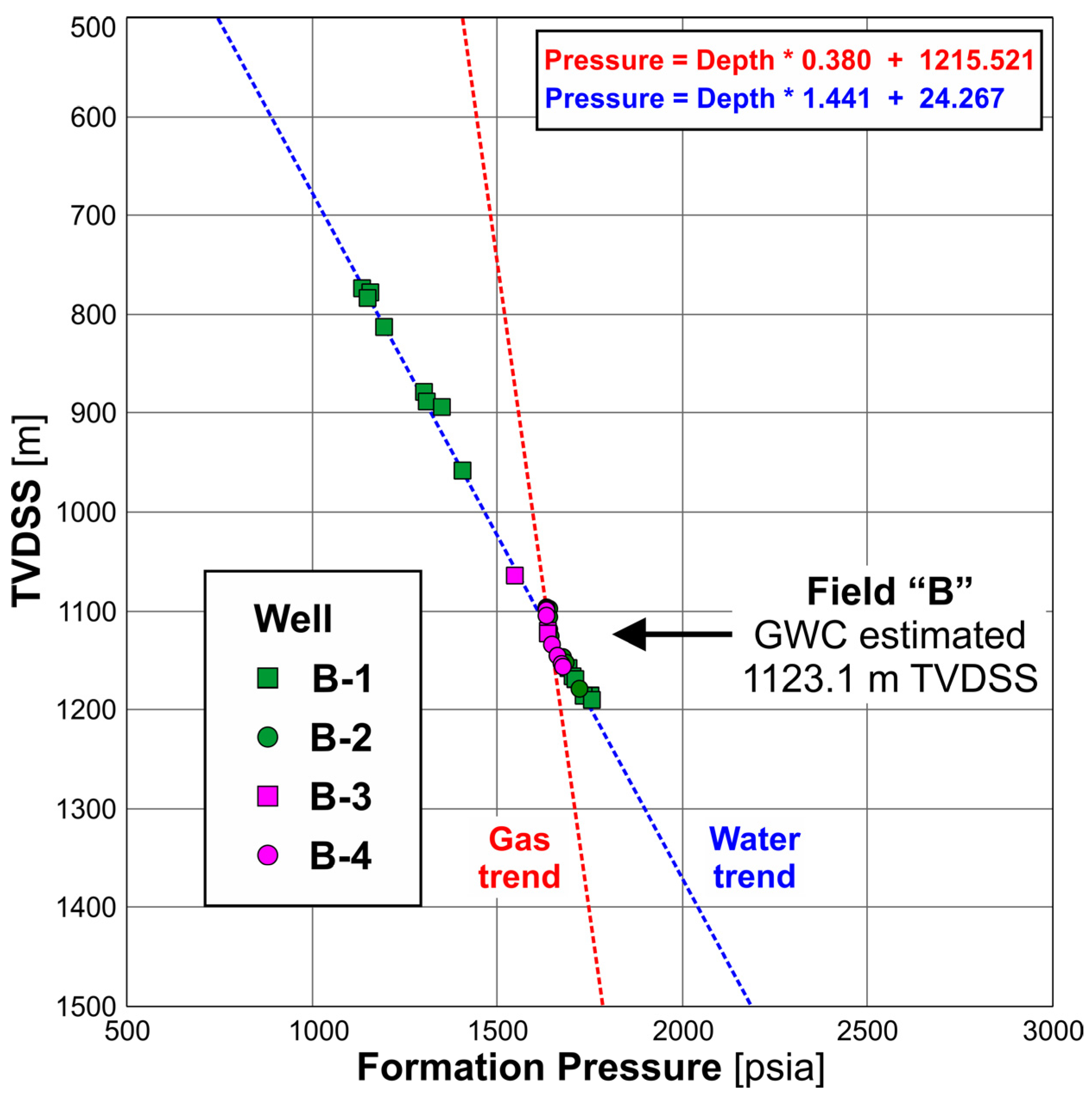
• The estimation of GWC depths using formation pressure surveys (frequently considered the main and preferred source of data for defining the fluid contacts) should always be checked and validated using the well log interpretation results. There is a significant degree of uncertainty in using the hydrostatic pressure trends identified in the analyzed wells to estimate the fluid contact position, due to the possibility that the pressures read by the wireline testers are not representative of formation water and gas, but might reflect mixtures of water (or mud filtrate) and gas in various ratios. The NMR log recorded in well A-2 provided valuable insight into the intervals with free fluids and with bound (immobile) water and allowed an assessment of the pressure-derived GWC validity;
• The well log interpretation results indicate that the Dacian reservoirs from fields “A” and “B” cannot be treated as single units, because they include two distinct reservoir intervals separated by permeability barriers of various thicknesses. Consequently, separate fluid contacts should be considered for each reservoir interval, instead of a single GWC obtained from the pressure gradients analysis.

References

1. Robinson, A.; Spadini, G.; Cloetingh, S.; Rudat, J. Stratigraphic evolution of the Black Sea: Inferences from basin modelling. Mar. Pet. Geol. 1995, 12, 821–835. [Google Scholar] [CrossRef]
2. Robinson, A.G.; Rudat, J.H.; Banks, C.J.; Wiles, R.L.F. Petroleum geology of the Black Sea. Mar. Pet. Geol. 1996, 13, 195–223. [Google Scholar] [CrossRef]
3. Moroşanu, I.C. Extensional Tectonics in the Tertiary of the Black Sea Shelf—Romanian Offshore. Geo-Eco-Marina 1998, 3, 153–158. [Google Scholar]
4. Moroşanu, I.C. Romanian Continental Plateau of the Black Sea: Tectonic-Sedimentary Evolution and Hydrocarbon Potential; Oscar Print: Bucharest, Romania, 2007; 176p, ISBN 978-973-668-167-X. [Google Scholar]
5. Moroşanu, I.C. The hydrocarbon potential of the Romanian Black Sea continental plateau. Rom. J. Earth Sci. 2012, 86, 91–109. [Google Scholar]
6. Dinu, C.; Wong, H.K.; Ţambrea, D.; Maţenco, L. Stratigraphic and structural characteristics of the Romanian Black Sea shelf. Tectonophysics 2005, 410, 417–435. [Google Scholar] [CrossRef]
7. Bega, Z.; Ionescu, G. Neogene structural styles of the NW Black Sea region, offshore Romania. Lead. Edge 2009, 28, 1082–1089. [Google Scholar] [CrossRef]
8. Crânganu, C.; Villa, M.A.; Şaramet, M.; Zakharova, N. Petrophysical Characteristics of Source and Reservoir Rocks in the Histria Basin, Western Black Sea. J. Pet. Geol. 2009, 32, 357–372. [Google Scholar] [CrossRef]
9. Georgiev, G. Geology and Hydrocarbon Systems in the Western Black Sea. Turkish J. Earth Sci. 2012, 21, 723–754. [Google Scholar]
10. Tari, G.; Bega, Z.; Fallah, M.; Kosi, W.; Krézsek, C.; Schléder, Z. The opening of the Western Black Sea Basin: An overview. In Proceedings of the 19th International Petroleum and Natural Gas Congress and Exhibition of Turkey, Ankara, Turkey, 15–17 May 2013. [Google Scholar] [CrossRef]
11. Nikishin, A.M.; Okay, A.I.; Tüysüz, O.; Demirer, A.; Amelin, N.; Petrov, E. The Black Sea basins structure and history: New model based on new deep penetration regional seismic data. Part 1: Basins structure and fill. Mar. Pet. Geol. 2015, 59, 638–655. [Google Scholar] [CrossRef]
12. Nikishin, A.M.; Okay, A.; Tüysüz, O.; Demirer, A.; Wannier, M.; Amelin, N.; Petrov, E. The Black Sea basins structure and history: New model based on new deep penetration regional seismic data. Part 2: Tectonic history and paleogeography. Mar. Pet. Geol. 2015, 59, 656–670. [Google Scholar] [CrossRef]
13. Oaie, G.; Seghedi, A.; Rădulescu, V. Natural marine hazards in the Black Sea and the system of their monitoring and real-time warning. Geo-Eco-Marina 2016, 22, 5–28. [Google Scholar]
14. Boote, D.R.D. The geological history of the Istria ‘Depression’, Romanian Black Sea shelf: Tectonic controls on second-/third-order sequence architecture. In Petroleum Geology of the Black Sea; Special Publications; Simmons, M.D., Tari, G.C., Okay, A.I., Eds.; Geological Society: London, UK, 2018; Volume 464, pp. 169–209. [Google Scholar]
15. Niculescu, B.M.; Andrei, G. Formation evaluation challenges in Pliocene gas-bearing reservoirs from the Romanian Western Black Sea shelf. E3S Web Conf. 2018, 66, 01004. [Google Scholar] [CrossRef]
16. Babskow, A.; Băleanu, I.; Popa, D.; Platon, V.; Mănescu, A. Results Concerning the Use of Seismic and Well Log Data for Defining the Geological Model of the Productive Structures on the Romanian Continental Shelf of the Black Sea. In Proceedings of the AAPG International Convention and Exposition Meeting, Nice, France, 10–13 September 1995. [Google Scholar]
17. Riedel, M.; Freudenthal, T.; Bergenthal, M.; Haeckel, M.; Wallmann, K.; Spangenberg, E.; Bialas, J.; Bohrmann, G. Physical properties and core-log seismic integration from drilling at the Danube deep-sea fan, Black Sea. Mar. Pet. Geol. 2020, 114, 104192. [Google Scholar] [CrossRef]
18. Stephenson, R.; Schellart, W.P. The Black Sea back-arc basin: Insights to its origin from geodynamic models of modern analogues. In Sedimentary Basin Tectonics from the Black Sea and Caucasus to the Arabian Platform; Special Publications; Sosson, M., Kaymakci, N., Stephenson, R.A., Bergerat, F., Starostenko, V., Eds.; Geological Society: London, UK, 2010; Volume 340, pp. 11–21. [Google Scholar]
19. Săndulescu, M. Geotectonics of Romania; Technical Publishing House: Bucharest, Romania, 1984; 336p. (In Romanian) [Google Scholar]
20. Săndulescu, M. Structure and Tectonic History of the Northern Margin of Tethys between the Alps and the Caucasus. In Evolution of the Northern Margin of Tethys: The Results of IGCP Project 198; Rakus, M., Dercourt, J., Nairn, A.E.M., Eds.; Société géologique de France: Paris, France, 1989; pp. 3–16. [Google Scholar]
21. Mutihac, V. Geological Structure of the Romanian Territory; Technical Publishing House: Bucharest, Romania, 1990. (In Romanian) [Google Scholar]
22. Bateman, R.M. Openhole Log Analysis and Formation Evaluation, 2nd ed.; Society of Petroleum Engineers: Richardson, TX, USA, 2012; 653p, ISBN 978-1-61399-269-2. [Google Scholar]
23. Klinkenberg, L.J. The permeability of porous media to liquids and gas. In Proceedings of the Drilling and Production Practice, New York, NY, USA, 1 January 1941; paper API-41-200. pp. 200–213. [Google Scholar]
24. Archie, G.E. The Electrical Resistivity Log as an Aid in Determining Some Reservoir Characteristics. Trans. Am. Inst. Min. Metall. Pet. Eng. 1942, 146, 54–62. [Google Scholar] [CrossRef]
25. Schlumberger Ltd. Log Interpretation Principles/Applications; Schlumberger Educational Services: Houston, TX, USA, 1991. [Google Scholar]
26. Hingle, A.T. The use of logs in exploration problems. In Proceedings of the SEG 29th International Annual Meeting, Los Angeles, CA, USA, 9–12 November 1959. [Google Scholar]
27. Asquith, G.; Krygowski, D. Basic Well Log Analysis, 2nd ed.; AAPG: Tulsa, OK, USA, 2004; 244p, ISBN 0-89181-667-4. [Google Scholar]
28. Pickett, G.R. Pattern Recognition as a Means of Formation Evaluation. Log Anal. 1973, 14, 3–11. [Google Scholar]
29. Coates, G.R.; Xiao, L.; Prammer, M.G. NMR Logging Principles and Applications; Halliburton Energy Services: Houston, TX, USA, 1999; 235p. [Google Scholar]
30. Mao, Z.Q.; Xiao, L.; Wang, Z.N.; Jin, Y.; Liu, X.G.; Xie, B. Estimation of permeability by integrating nuclear magnetic resonance (NMR) logs with mercury injection capillary pressure (MICP) data in tight gas sands. Appl. Magn. Reson. 2013, 44, 449–468. [Google Scholar] [CrossRef]
31. Spooner, P. Lifting the Fog of Confusion Surrounding Clay and Shale in Petrophysics. In Proceedings of the SPWLA 55th Annual Logging Symposium, Abu Dhabi, United Arab Emirates, 18–22 May 2014. paper SPWLA-2014-VV. [Google Scholar]
32. Schlumberger Ltd. Log Interpretation Charts; Schlumberger Ltd.: Houston, TX, USA, 2013; ISBN 978-1-937949-10-5. [Google Scholar]
33. Serra, O. Well Logging and Reservoir Evaluation; Editions Technip: Paris, France, 2007; ISBN 978-2-7108-0881-7. [Google Scholar]
34. Poupon, A.; Leveaux, J. Evaluation of water saturation in shaly formations. Log Anal. 1971, 12, 3–8. [Google Scholar]
35. Heslop, A. Gamma-ray log response of shaly sandstones. In Proceedings of the SPWLA 15th Annual Logging Symposium, McAllen, TX, USA, 2–5 June 1974. paper SPWLA-1974-M. [Google Scholar]
36. Katahara, K.W. Gamma Ray Log Response in Shaly Sands. Log Anal. 1995, 36, 50–56. [Google Scholar]
37. Ellis, D.W.; Singer, J.M. Well Logging for Earth Scientists, 2nd ed.; Springer: Dordrecht, The Netherlands, 2008; 692p, ISBN 978-1-4020-4602-5. [Google Scholar]
Figure 1. Simplified map of the Romanian Black Sea shelf indicating the main plays, leads and structural–tectonic elements. 1—Pelican, 2—Sfântul Gheorghe, 3—Sacalin, 4—Sturion, 5—Egreta, 6—Portiţa, 7—Heracleea, 8—Venus, 9—Sinoe, 10—Lebăda West, 11—Lebăda East, 12—Minerva, 13—Albatros, 14—Iris, 15—Lotus, 16—Tomis, 17—Ovidiu, 18—Cobălcescu, 19—Vadu, 20—Corbu, 21—Midia, 22—Meduza, 23—Neptun, 24—Neptun East, 25—Delfin, 26—Jupiter, 27—Pescăruş, 28—Doina, 29—Ana, 30—Muridava (Olimpyska), 31—Domino, 32—Eugenia. SGF—Sfântul Gheorghe fault, PCF—Peceneaga–Camena fault, COF—Capidava–Ovidiu fault, IMF—Intramoesian fault, RF—Razelm fault, LRF—Lacul Roşu fault, HF—Heracleea fault. A–A’—Geological cross-section. (adapted from [4,5,13,15]).
Energies 14 06629 g001
Figure 2. A–A’ Geological cross-section with W–E direction through the Romanian Black Sea shelf area, based on seismic reflection and well data (redrawn and modified from [9]).
Energies 14 06629 g002
Figure 3. Example of wireline geophysical logs recorded in an exploration well (A-2) from the Early Pliocene gas field “A” (adapted from [15]).
Energies 14 06629 g003
Figure 4. Example of wireline geophysical logs recorded in an exploration well (B-4) from the Early Pliocene gas field “B” (adapted from [15]).
Energies 14 06629 g004
Figure 5. Neutron–density crossplot corresponding to the Pliocene (“Sand”, “Silt”, and post-reservoir) deposits of field “A” and including data from A-1 and A-2 wells (7180 data levels). A caliper cut-off (d < 9 in) was used to eliminate the bad hole levels. The approximate location of a clay point (ϕNclay, ρclay) representative for the entire Pliocene sequence is indicated. SS, LS, and DOL are theoretical ρb = f(ϕN) response curves for the main reservoir lithologies (sandstone, limestone, dolomite) [32].
Energies 14 06629 g005
Figure 6. Volumetric representation of the “shaly sands” petrophysical model adopted for the quantitative interpretation of well logs.
Energies 14 06629 g006
Figure 7. Clay volume derived from GR log (track 4) and from the neutron–density logs combination (track 6). VclayGR (track 5) is referenced against the ϕNclayϕDclay separation (tracks 6 and 7) to provide VclayGRVclayND in the shaly water-bearing intervals (track 8) and is used as the final clay indicator (track 9). TNPH_SS is the matrix-corrected (sandstone) neutron log.
Energies 14 06629 g007
Figure 8. Estimation of fluid contact depths by means of formation pressure measurements, even if the actual contact is not intercepted by exploration wells.
Energies 14 06629 g008
Figure 9. (a) Core permeability–core porosity relationship for the pre-reservoir, “Sand”, “Silt”, and post-reservoir deposits of “A” and “B” fields; (b) NMR permeability–gamma ray intensity dependence for the same sequence of deposits in the A-2 well (567 data levels). The color code corresponds to Sw values resulting from the petrophysical interpretation of well logs.
Energies 14 06629 g009
Figure 10. Hingle-type resistivity–porosity crossplots based on log-derived density porosity (ϕD) and parameters (ρma, m, n) obtained from core analyses (RCAL and SCAL). (a) B-2 well (528 data levels), showing water-bearing intervals with large porosity and resistivity range; (b) B-4 well (581 data levels), showing water-bearing intervals with narrow porosity and resistivity range.
Energies 14 06629 g010
Figure 11. Pickett-type resistivity–porosity crossplots based on the effective porosity (ϕe) resulted from well log interpretation and parameters (ρma, m, n) obtained from core analyses (RCAL and SCAL). (a) B-3 well (2080 data levels); (b) B-3 well with a gamma-ray cut-off applied (GR < 70 gAPI) (113 data levels).
Energies 14 06629 g011
Figure 12. Pickett-type resistivity–porosity crossplots based on the effective porosity (ϕe) resulting from well log interpretation and parameters (ρma, m, n) obtained from core analyses (RCAL and SCAL). (a) A-1 well (681 data levels); (b) A-2 well (933 data levels).
Energies 14 06629 g012
Figure 13. Example of deterministic log interpretation results for well A-1. HTEM—borehole temperature, GR—gamma-ray intensity, HCAL—caliper, BS—bit size, RLA5—deep Laterolog apparent resistivity, RoRec—reconstructed R0 resistivity, SW—uninvaded zone water saturation, SXO—flushed zone water saturation, PHIE—effective porosity, BVW—uninvaded zone bulk volume of water, BVWSXO— flushed zone bulk volume of water, VWCL—wet clay volume, VSILT—silt volume (silt index), PRES—formation pressure readings, CORE_SW—core-derived water saturation, CORE_PHI—core-derived porosity, CORE_K—core-derived permeability, C1—cored interval.
Energies 14 06629 g013
Figure 14. Example of deterministic log interpretation results for well A-2. HTEM—borehole temperature, GR—gamma-ray intensity, HCAL—caliper, BS—bit size, RLA5—deep Laterolog apparent resistivity, RoRec—reconstructed R0 resistivity, SW—uninvaded zone water saturation, SXO—flushed zone water saturation, PHIE—effective porosity, BVW—uninvaded zone bulk volume of water, BVWSXO— flushed zone bulk volume of water, VWCL—wet clay volume, VSILT—silt volume (silt index), T2_NORM—normalized NMR T2 distribution, NMR_PHIT—NMR total porosity, NMR_PHIE—NMR effective porosity, NMR_FFI—NMR Free Fluid Index, NMR_K—Permeability derived from NMR, PRES—formation pressure readings. The upward arrow indicates a possible active gas migration from deeper levels.
Energies 14 06629 g014
Figure 15. Example of deterministic log interpretation results for well B-2. TEMP—borehole temperature, GR—gamma-ray intensity, CAL—caliper, BS—bit size, RLLD—deep Laterolog apparent resistivity (≈ Rt), RoRec—reconstructed R0 resistivity, SW—uninvaded zone water saturation, SXO—flushed zone water saturation, PHIE—effective porosity, BVW—uninvaded zone bulk volume of water, BVWSXO— flushed zone bulk volume of water, VWCL—wet clay volume, VSILT—silt volume (silt index), MLR_K—predicted permeability from Multiple Linear Regression analysis, CORE_K—core-derived permeability, PRES—formation pressure readings, C1–C4—cored intervals. The upward arrow indicates a possible active gas migration from deeper levels.
Energies 14 06629 g015
Figure 16. Estimation of gas–water contact (GWC) for field “A” by jointly using pressure measurements from available wells.
Energies 14 06629 g016
Figure 17. Estimation of gas–water contact (GWC) for field “B” by jointly using pressure measurements from available wells.
Energies 14 06629 g017