The Carbon Dioxide Emission as Indicator of the Geothermal Heat Flow: Review of Local and Regional Applications with a Special Focus on Italy

Abstract

We review the methods based on the measurement of CO₂ emissions for the computation of geothermal heat flow, both at a local (hydrothermal sites, a few km²) and regional scale (hundreds km²). At the local scale, we present and discuss the cases of the Latera caldera and Torre Alfina (Italy) geothermal systems. At Torre Alfina and Latera, the convection process sustains a CO₂ emission of ~1 kg s⁻¹ and ~4 kg s⁻¹, and heat flows of 46 MW and 130 MW, respectively. At the regional scale, we discuss the case of the central Apennine (Italy), where CO₂ mass and enthalpy balances of regional aquifers highlights a wide and strong thermal anomaly in an area of low conductive heat flow. Notably, the CO₂/heat ratios computed for the central Apennines are very similar to those of the nearby geothermal systems of Latium and Tuscany, suggesting a common source of CO₂-rich fluids ascribed to the Tyrrhenian mantle.

1. Introduction

Since the late seventies numerous studies have pointed to high carbon dioxide emissions in tectonically active regions frequently hosting geothermal systems [1,2,3]. High-temperature geothermal systems form in active magmatic regions, where a large amount of heat is lost from the Earth’s interior. The heat and mass transfer from a cooling magmatic intrusion to the groundwater drives fluid convection, boiling, and steam separation [4]. In the low-permeability and high-temperature ductile rocks hosting the intrusion, the heat transfer is dominated by conduction. Contrarily, convection dominates heat transfer in the permeable rocks of geothermal systems. The boiling of the convecting liquids produces a vapor-dominated phase with a significant amount of CO₂, which flows towards the surface. Consequently, geothermal regions represent prevalent emitters of both geogenic CO₂ and heat [5,6,7,8,9].

In these areas, CO₂ is either emitted in the atmosphere through focused fumarolic vents, boiling pools, and areas of diffuse soil degassing [10,11,12], or dissolved in groundwater [13,14]. In the late 1990s, Kerrick et al. [5] developed a methodology based on convective heat flow measurements to estimate the relative flux of CO₂ from geothermal systems. Subsequently, the development of techniques for measuring CO₂ fluxes from volcanic and geothermal soil, such as the accumulation chamber [15] and eddy covariance [16], enabled the convective heat flow to be estimated by applying the reverse approach.

The aim of this study was to synthesize in a unique document the principles and results of CO₂-based techniques for the estimation of heat flow, referring to published and unpublished cases. In detail we will show how the measurement of soil CO₂ degassing can be used to compute both the thermal emission from the hot soils of hydrothermal sites and the total heat associated with the convection of geothermal liquids. The published results obtained at Latera caldera (Italy) are presented and discussed together with those obtained from unpublished CO₂ flux measurements performed at the Torre Alfina geothermal area (Italy). These cases show that CO₂ flux measurements find useful applications in geothermal prospecting because they allow one to cheaply estimate the natural advective-convective heat flow.

Finally, we re-elaborated the published data of a regional investigation on the aquifers of the central Apennine (Italy) [17] computing, aquifer by aquifer, the total deeply derived CO₂ emission and the geothermal heat flow from these hundreds of square kilometers wide areas. The results, supported by the CO₂ concentrations and enthalpies of geothermal fluids of the region, indicate the presence of a geothermal source particularly rich in CO₂ in central Italy.

2. Geothermal Heat Flow from the Diffuse Emission of CO₂

According to [5], in geothermal systems heat and CO₂ are transferred from depth to the surface through the convection of geothermal liquids (Figure 1). Based on this conceptual model, Kerrick et al. [5] used the heat flow measured at the surface to calculate the CO₂ emission from the Taupo geothermal zone (New Zealand). Assuming the same conceptual model, in reverse the measured emission of CO₂ can be used to compute the thermal energy of the upflowing geothermal fluids.

Considering that the CO₂ flow towards the surface (Q_CO2 in kg s⁻¹) is sustained by the depressurization and boiling of the geothermal liquid during its upflow (Figure 1), the mass flow rate of the liquid (Q_L in kg s⁻¹) and the associated thermal energy (Q_H in MW) can be computed, rearranging the original relation of [5] as:

Q_L = Q_CO2/(m_CO2 × 0.044)

(1)

Q_H = 10⁻³ × Q_L × H_L

(2)

where H_L (in kJ kg⁻¹) is the original enthalpy of the liquid, m_CO2 (in mol kg⁻¹) is the original CO₂ concentration, and 0.044 is the factor to convert moles to kg. During the boiling of the upflowing liquid, the original energy is divided into a fraction associated with the residual liquid, which is possibly discharged by thermal springs or returned into the system with the descending columns of convective cells (Q_res and Q_H,res in Figure 1), and a fraction transported toward the surface by the separated vapor. This ascending vapor-dominated phase condenses near the surface heating the soil, whereas the low-soluble CO₂ is emitted in the atmosphere.

According to this model, geothermal areas often host sites characterized by emissions of hydrothermal CO₂ from hot soils (steaming ground), which extend over their fumarolic fields. To measure the heat flow from these hot soils, several techniques have been developed since the 1950s [18] (and references therein). In these pioneer works, the heat flow is calculated by measuring soil temperatures at fixed depths and using empirical relations derived from long, time-consuming heat flow measurements with suitable calorimeters. For example, Fridriksson et al. [10] following [18], proposed that q_s = 5.2 × 10⁻⁶ × t₁₅⁴, where q_s is the heat flow (in W m⁻²) and t₁₅ is the soil temperature (in °C) at a depth of 15 cm. However, this method is not generally valid because the empirically derived relation depends on local conditions, such as soil thermal conductivity and ambient temperature.

More recently Chiodini et al. [6,19] proposed an approach based on the measurement of the diffuse emission of hydrothermal CO₂ from hot soils. In this approach the equivalent amount of steam that condenses in the subsurface (Q_cond in kg s⁻¹) and the associated heat release (Q_H,cond in MW) is computed using the following equations:

Q_cond = Q_CO2 × R_H2O/CO2

(3)

Q_H,cond = 10⁻³ × Q_cond × (H_{V, Tcond} − H_{L, Tamb})

(4)

where R_H2O/CO2 is the H₂O/CO₂ weight ratio of the original (precondensation) vapor phase, and H_{V, Tcond} and H_{L, Tamb} are the enthalpies of the steam at the condensation temperature (2676 kJ kg⁻¹ for a condensation temperature of 100 °C; [20]) and of the liquid at the ambient temperature (83.9 kJ kg⁻¹ for an ambient temperature of 20 °C; [20]), respectively. These equations are solved assuming a R_H2O/CO2 equal to that of the fumaroles located in the zone degassing CO₂ [6].

In the next sections we present and discuss the results obtained in different hydrothermal areas where Q_CO2 is used for the estimation of Q_H,cond and Q_H.

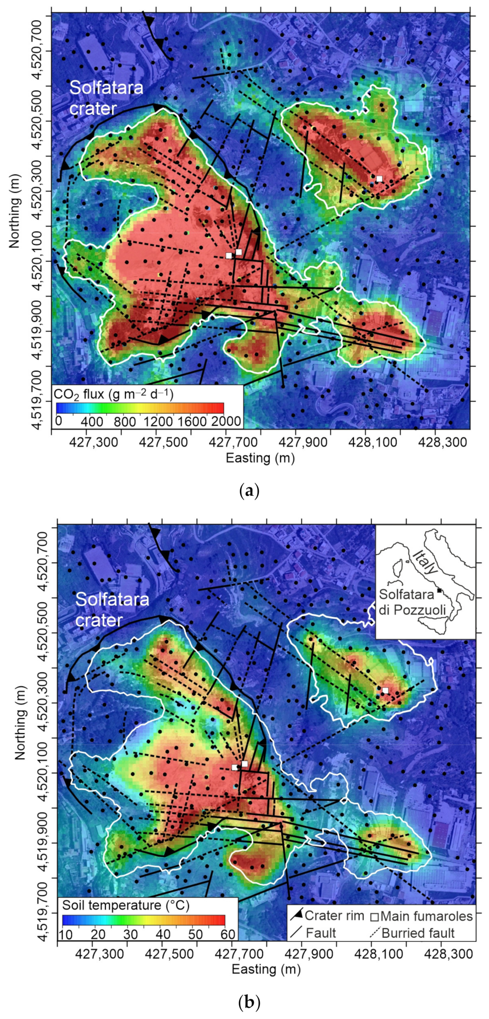
2.1. Thermal Energy Release from Soils Heated by Steam Condensation (Q_H,cond)

The approach based on the application of Equations (3) and (4) is strongly supported by the spatial correspondence between hot soils and CO₂ emissions, which frequently characterize the hydrothermal areas of active volcanoes and geothermal sites. Figure 2 shows, e.g., the map of CO₂ fluxes and soil temperature (at 10 cm of depth) of the Solfatara di Pozzuoli (Campi Flegrei caldera, Italy), where this approach was first tested in 1998 [19]. These maps, as well as those reported in the following figures, were elaborated using the sequential Gaussian simulations (sGs; [21]) method. Equations (3) and (4) were solved with the measured Q_CO2 (17.6 kg s⁻¹) and R_H2O/CO2 (2.2) obtaining the energy released by steam condensation from the Solfatara di Pozzuoli (Q_H,cond~100 MW, [19]). This thermal energy was released from an area of ~0.5 km² (

Table 1. Thermal energy associated with the CO₂ degassing from hot soils from some geothermal/hydrothermal systems and relevant parameters for its calculation.

Volcano (DDS)	Date	DDS Extent a km2	RH2O/CO2	QCO2 kg s−1	Qcond kg s−1	QH,cond MW	Reference
Campi Flegrei, Solfatara	12/1998	0.454 b	2.20	17.6	38.72	100.4	[19]
Campi Flegrei, Solfatara	07/2000	0.455 b	2.27	17.13	38.88	100.8	[6]
Ischia, Donna Rachele	04/2001	0.058	147	0.11	15.48	40.1	[6]
Vesuvio, cone	04/2000	0.331	3.66	1.75	6.40	16.6	[6]
Vulcano, crater	07/1998	0.415	4.42	1.83	8.08	21.0	[6]
Vulcano, PL Beach	03/2002	0.018	5.24	0.22	1.15	3.0	[6]
Pantelleria, Favara Grande	07/2004	0.058	17.2	0.08	1.39	3.6	[6]
Masaya, Comalito	03/2003	0.010	1.60	0.22	0.35	0.9	[6]
Yellowstone, Mud volcanoes	08/2003	0.400	3.49	3.36	11.82	30.6	[6]
Yellowstone (HSB)	-	0.160	15.63	0.80	12.48	32.3	[23]
Yellowstone (HLGB)	-	0.040	250	0.02	5.79	15.0	[23]
Yellowstone (CH)	08/2014	<0.035 c	13.44	0.97	13.1	33.9	[24]
Nisyros-Stefanos	10/2018	0.086	36.0	0.19	7.00	18.1	[25]
Nisyros-Kaminakia	10/2018	0.164	6.90	0.16	1.08	2.8	[25]
Nisyros-Polibote	10/2018	0.031	26.0	0.07	1.68	4.4	[25]
Nisyros-Phlegeton	10/2018	0.053	21.2	0.04	0.85	2.2	[25]
Nisyros Lofos	10/2018	0.196	27.3	0.23	6.31	16.4	[25]
Nisyros-Ramos	10/2018	0.048	16.5	0.12	2.01	5.2	[25]
Nisyros-NEfault	10/2018	0.124	6.9	0.10	0.66	1.7	[25]
Nisyros-SENWline	10/2018	0.123	27.3	0.05	1.30	3.4	[25]
Nisyros-NESWline	10/2018	0.029	27.3	0.02	0.59	1.5	[25]
Nisyros, all DDSs	10/2018	0.825	6.9–36	1.06	23.40	60.7	[25]
Nisyros, all DDSs	02/2000	0.690	6.1–36	0.79	16.44	42.6	[26]
Copahue-Las Máquinas	03/2014	<0.321 c	15.8	0.43	6.73	14.9	[27]
Copahue-Las Maquinitas I+II	03/2014	<0.079 c	17.3	0.19	3.30	7.3	[27]
Termas Copahue	03/2014	<0.576 c	16.6	1.05	17.45	38.7	[27]
Terceira-Furnas do Enxofre	08/2014	<0.024 c	14.9	0.03	0.44	1.1	[28]
Teide	07/2016	<0.560 c	2.24	2.44	5.47	14.2	[29]
Peteroa	01/2020	<0.08 c	12.9	0.08	0.77	2.6	[30]

^a For the criteria used to define the DDS extent see the original works; ^b DDS extent from [22]; ^c survey areas are reported when DDS extent is not defined in the original works.

) and constituted the main part of the total energetic budget of the Campi Flegrei caldera. In fact, it was much higher than (i) the conductive heat flux over the ~100 km² of the entire caldera, (ii) the energy of the earthquakes, and (iii) the energy associated with ground deformation [19]. Subsequently, this method was applied to many geothermal sites in the world. Some examples and their relative references are reported in Table 1, where the acronym DDS (Diffuse Degassing Structure) indicates the areas diffusively emitting the hydrothermal, deeply derived CO₂. The cases reported in Table 1 were selected based on the availability of (i) detailed CO₂ flux surveys, (ii) estimation of the deeply derived emission (note that in the literature often is reported the total emission but not that related to the deep source), and (iii) the composition of the fumaroles located in the area.

2.2. Thermal Energy of Convective Geothermal Liquid (Q_H)

In

Table 2. Thermal energy associated with the convection of geothermal fluids. The cases were selected based on the availability of T_L and m_CO2 of the original geothermal liquid.

Name	QCO2 kg s−1	mCO2 mol kg−1	TL °C	HL kJ kg−1	QL kg s−1	QH MW
Reykjanes 1	0.156	0.0284	290	1289	125	161
Nisyros 2	1.060	0.29	340	1594	83.9	134
Torre Alfina	1.064	0.33	150	632.2	73.3	46
Latera	4.050	0.73	238	1028	126.1	130

¹ data from [10]; ² data from [25].

we report some results of the method for the estimation of the total thermal energy Q_H involved in the convective generation of gas emissions (Figure 1) using published [10,12,25] and unpublished data. Equations (1) and (2) were solved assuming H_L and m_CO2 of the hottest geothermal well as representative of the original convecting liquid. The computations completed at Latera caldera and Torre Alfina starting from the CO₂ emission measurements are then described in detail in the following sections. Latera and Torre Alfina are two geothermal systems located in the Quaternary volcanic region of central Italy [31] (and references therein) which emit a low-temperature and dry gas phase, dominated by CO₂. We use published measurements of the diffuse CO₂ emission at Latera [12], while, in the case of Torre Alfina we use unpublished data.

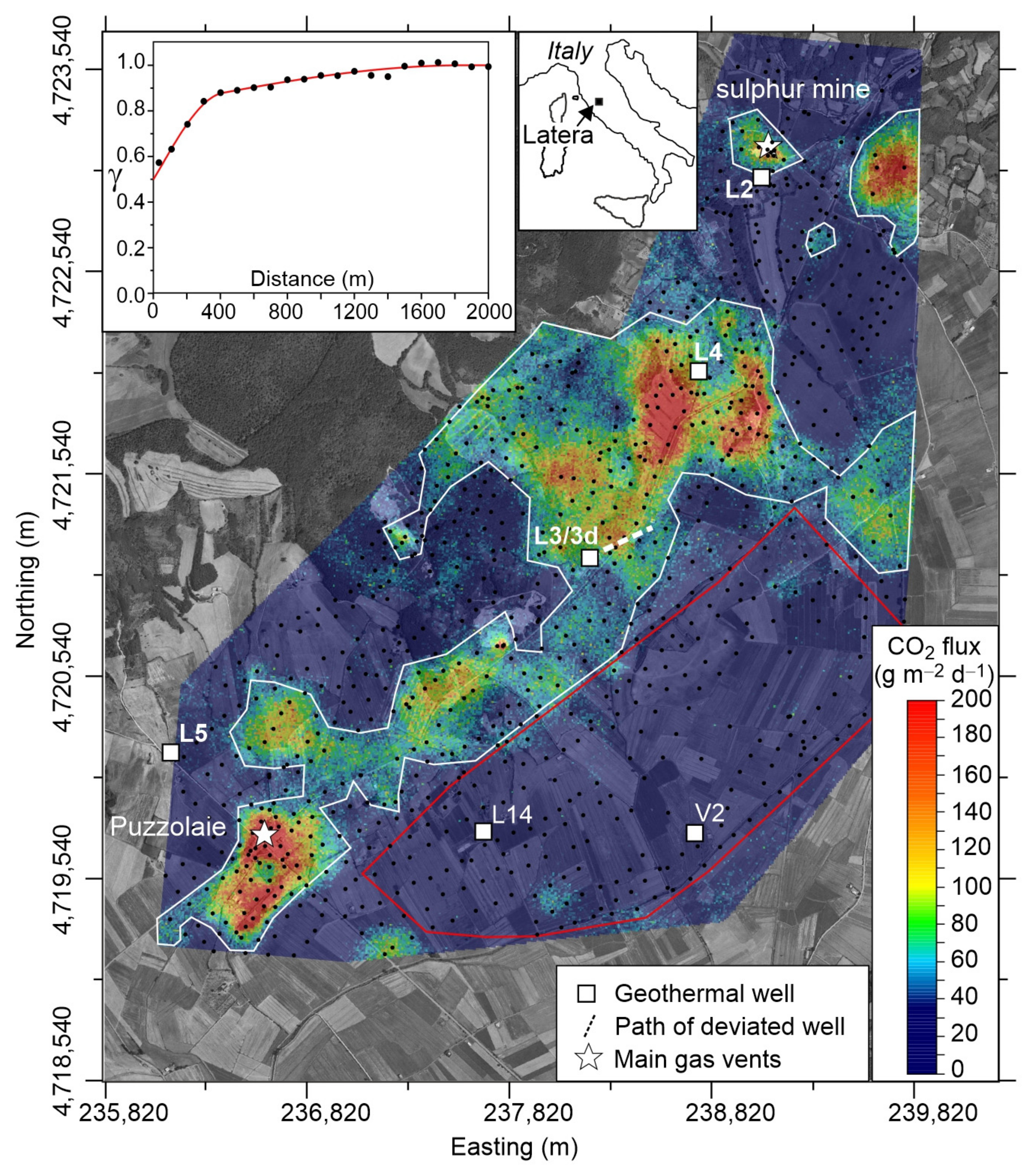
2.2.1. CO₂ Emission and Convective Heat Release from the Latera Caldera

Results of a detailed investigation of the CO₂ degassing from the Latera caldera [12] are here synthesized and discussed. The Latera geothermal system is hosted in permeable Mesozoic carbonates covered by impermeable flysch layers and volcanic products (see [12] for a detailed geological setting). Surface manifestations of the active fluid circulation consist of CO₂-rich shallow groundwaters, areas of strong soil diffuse CO₂ emission, and low-temperature (from 19 °C to 31 °C) CO₂-rich gas vents. The CO₂ emission was quantified and mapped through 930 flux measurements performed with the accumulation chamber over an area of ~10.8 km² (Figure 3; [12]). The CO₂ flux map shows a NE-SW band of high CO₂ emission (Latera DDS), corresponding to the structural high hosting the geothermal reservoir [12,32,33]. Notably, the productive wells of Latera (L3/3D, L2 and L4 in Figure 3) are located in this anomalous band.

The total CO₂ emission computed from the map resulted in 497 t d⁻¹, including both the geothermal and biogenic flux contributions. The mean soil biogenic production, which was characterized using a subset of measurements performed in an area far from the main degassing zones (red contour in Figure 3), resulted in 15.7 g m⁻² d⁻¹. Removing the biogenic CO₂ contribution, the deep CO₂ emission from Latera resulted in 328 t d⁻¹ [12]. Then, integrating this large-scale survey with the results of a detailed CO₂ flux campaign focused on the biggest gas manifestation in Latera, that is the Puzzolaie area, these authors concluded that the total deep CO₂ emission accounted for ~350 t d⁻¹ (4.05 kg s⁻¹).

The total thermal energy involved in the convective upflow and boiling of the geothermal liquids was calculated with Equations (1) and (2), using the published T-m_CO2 data of the hottest geothermal liquid (Latera 3D well, T = 238 °C, m_CO2 = 0.73 mol kg⁻¹; [34,35]). The geothermal fluid upflow rate (Q_L), feeding the CO₂ emission of 4.05 kg s⁻¹, resulted in 126 kg s⁻¹ and the correspondent thermal energy (Q_H) in 130 MW.

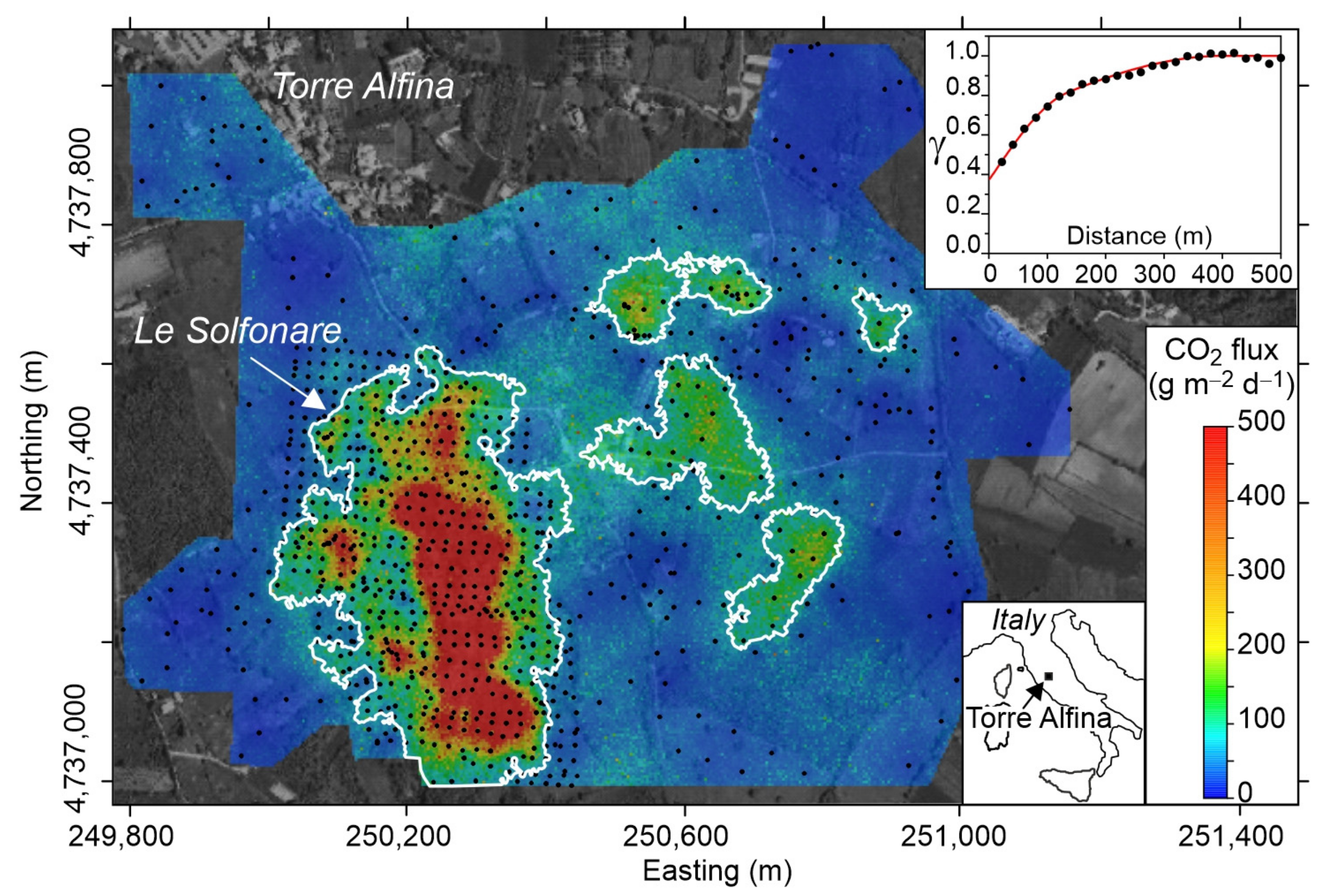
2.2.2. CO₂ Emission and Convective Heat Release from Torre Alfina, Italy

The Torre Alfina system consists of both a geothermal liquid water reservoir with temperatures between 125 and 150 °C and an overlying gas-cap, mainly CO₂, at a pressure of about 40 bars [36], located at ~400 m of depth. Similarly to Latera, the reservoir is hosted in a structural high of the Mesozoic carbonate formations overlaid by flysch impermeable layers and by quaternary volcanic products [36,37]. The area above the geothermal system is characterized by high pCO₂ groundwaters circulating in the volcanic products [38], CO₂-rich gas vents, and areas with visible soil CO₂ emissions. Soil CO₂ diffuse degassing was investigated with the accumulation chamber method [15] in 2009–2010. This survey consisted of (i) 917 CO₂ flux measurements performed in the main CO₂ emission area located southward of the Torre Alfina village (named “Le Solfonare” by [39]; Figure 4), (ii) 119 measurements in a peripheral area with slightly high flux values (named “small degassing area”), and (iii) 262 measurements of low CO₂ flux randomly distributed in a larger area and specifically performed to quantify the background soil CO₂ emissions (Table S1, Supplementary Material).

The CO₂ flux map of Le Solfonare, constructed with the sGs method [21], highlights a main NNW-SSE degassing structure and weaker anomalies located eastward (Figure 4). In total, these two anomalous zones emit 104.7 t d⁻¹ of CO₂, which become 107.0 t d⁻¹ summing the 2.3 t d⁻¹ released by the small degassing area. This value includes both the geothermal CO₂ and the background emission due to the biologic activity in the soil. To separate these two contributions, we applied the GSA (Graphic Statistic Approach described in [15] and in [21]), which is based on the Sinclair’s partitioning method of lognormal polymodal distribution of data [40]. The CO₂ flux measurements are reported in the log-probability plot of Figure 5 (grey points), where, for comparison, are also reported the 262 background values as a separated data set (blue points). The distribution of the CO₂ fluxes is explainable by the overlapping of the background population (defined only with the blue points) and two other lognormal populations of higher fluxes, representing the deep CO₂ contribution (

Table 3. Statistical parameters of the individual partitioned populations.

Population	Mean Log CO2 Flux	σ	%	Mean CO2 Flux * g m−2 d−1
1	1.05	0.30	33	14.2 (13.3–15.2)
2	1.62	0.29	46	52.1(49.4–54.8)
3	2.15	0.75	21	626 (441–905)

* The mean of the CO₂ flux was then estimated using a Monte Carlo simulation procedure. Between brackets are reported the 5th and 95th percentile of the mean CO₂ flux values returned by the Monte Carlo simulation procedure [41].

). Based on the statistical parameters of the Population 1, we estimate an average background CO₂ emission of 14.2 g m⁻² d⁻¹ which, interestingly, is very similar to the CO₂ background flux of Latera, closely located to Torre Alfina and characterized by a similar type of vegetation and use of soil. Considering this background CO₂ emission we estimate the total deep CO₂ emission at 91.9 t d⁻¹ (1.06 kg s⁻¹). We assume that 35 g m⁻² d⁻¹ (95th percentile of Population 1) reflects the threshold value above which the gas emission is totally geogenic-derived. This value is used to delimitate the structures degassing deeply derived CO₂ (Torre Alfina DDS, white contour in Figure 4).

The thermal energy involved in the upflow of the geothermal liquid of the Torre Alfina system was computed with Equations (1) and (2), considering temperature and m_CO2 data of the wells reported in [34]. Among these data we selected the maximum temperature (150 °C) at which corresponds a m_CO2 equal to 0.33 mol kg⁻¹. Considering the CO₂ diffuse emission of 1.06 kg s⁻¹, we estimated a geothermal fluid upflow (Q_L) equal to 73.2 kg s⁻¹ and an associated thermal energy (Q_H) equal to 46 MW.

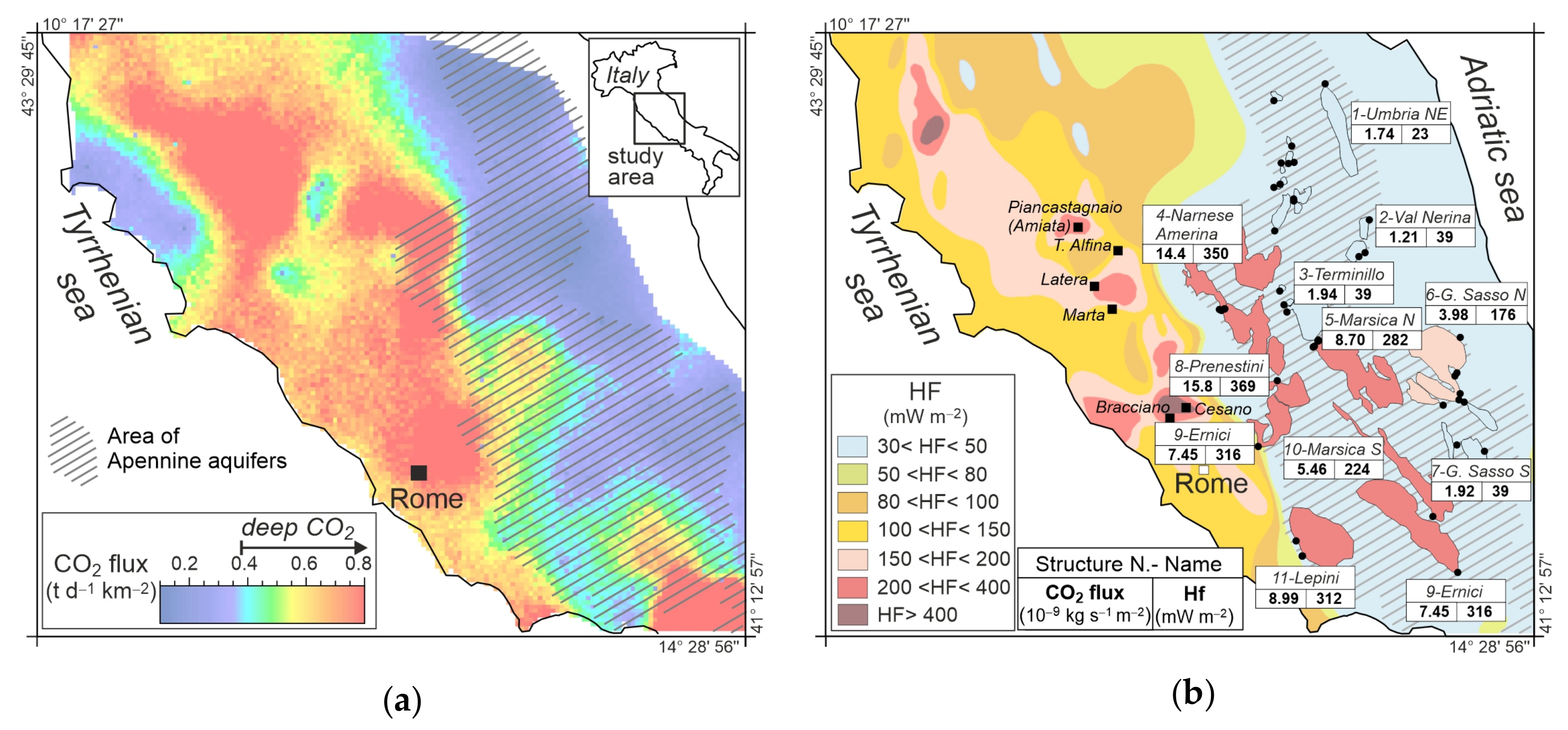
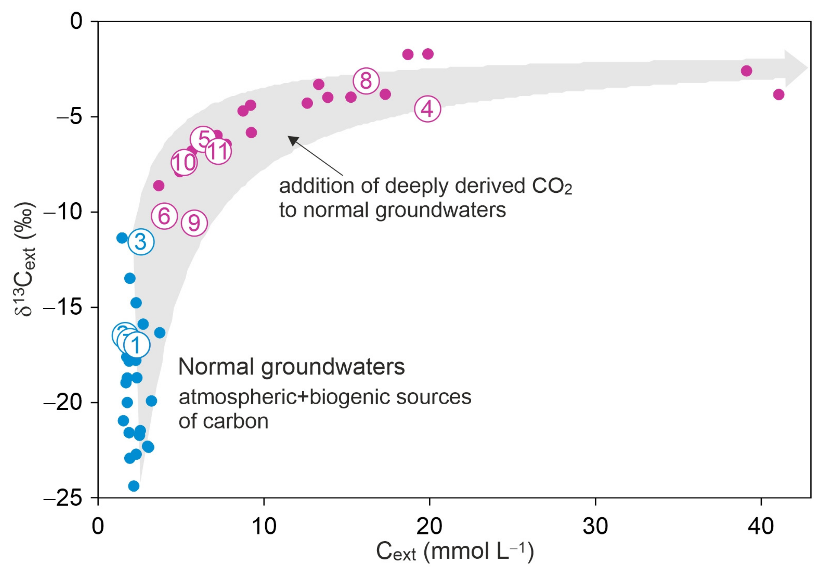
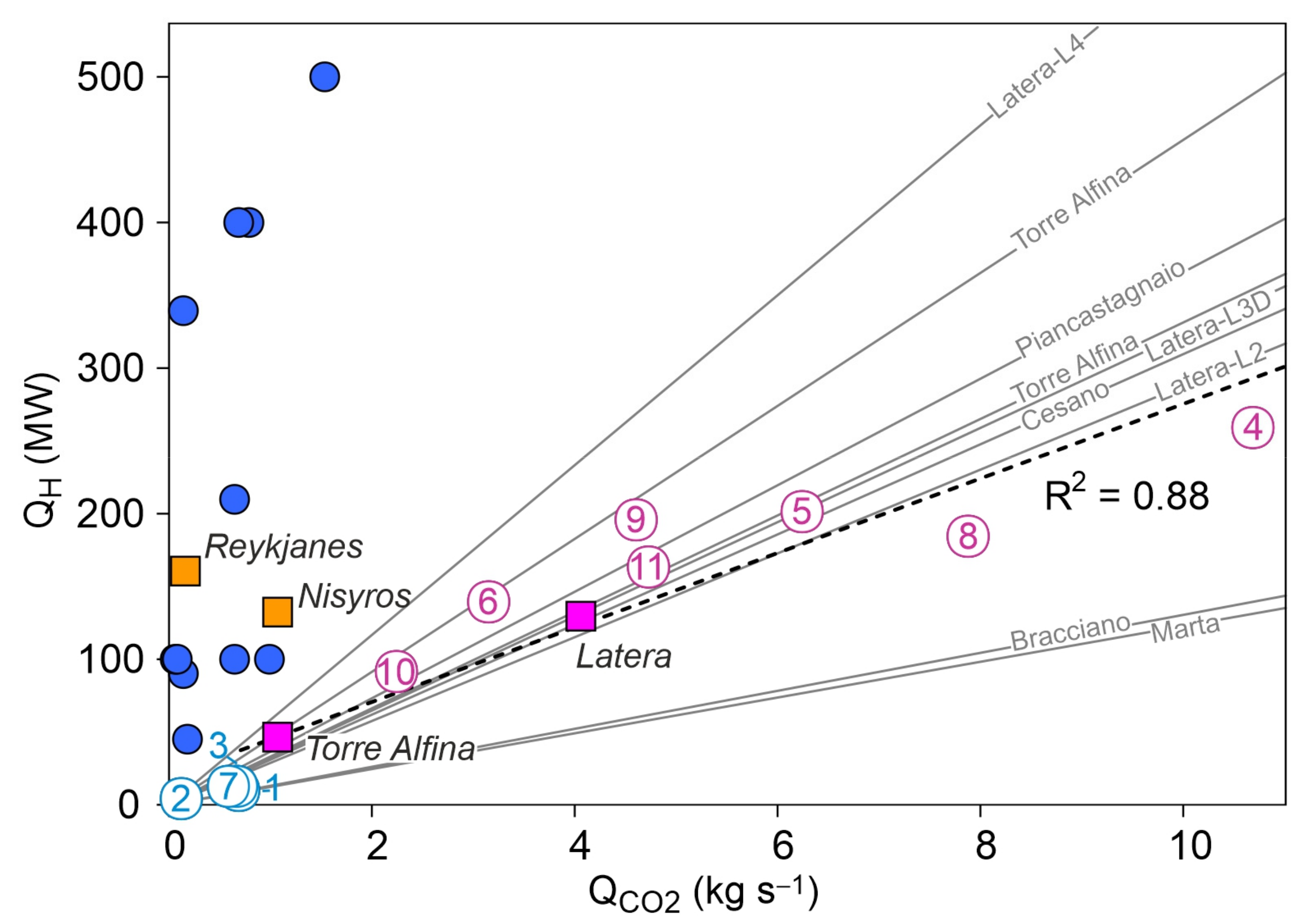
3. Enthalpy and CO₂ Mass Balances of Regional Aquifers

In the previous section we combined surface measurements of the CO₂ flux with the enthalpy and CO₂ content of deep liquids to calculate the heat release and the thermal energy of the geothermal fluids exsolving CO₂. When the upflowing fluids dissolve in aquifers, we do not need any direct information about the deep fluids to estimate the heat flux and the amount of injected CO₂, as they can be calculated through the carbon mass and enthalpy balances of groundwaters.

This approach was used in central Italy [17] where the comparison of the CO₂ flux map [42] with the conductive heat flux map [43] points out that the area of anomalous CO₂ degassing extends eastward beyond the thermal anomaly (Figure 6). The heat flux shows in fact a sharp decrease from values higher than 100 mW m⁻², typical of the Tyrrhenian side, to values lower than 50 mW m⁻² in the area of the regional aquifers of the Apennine chain. Here, the large amounts of infiltrating waters that circulate in the permeable carbonate formations possibly cools the crust and causes the low conductive heat flux measured in the area [17,44].

To investigate the heat transfer in this area, Chiodini et al. [17] applied carbon mass and enthalpy balances to 46 springs of high-flow rate located in 11 large carbonate aquifers (Figure 6b). The carbon mass balance of the springs allowed [17] to differentiate the components contributing to the total dissolved inorganic carbon (TDIC), i.e., the carbon deriving from carbonate minerals dissolution (C_carb) and that from sources external to the aquifers (C_ext).

The diagram of δ¹³C_ext vs. C_ext (Figure 7) highlights two groups of waters: one characterized by low C_ext (mean = 2.3 mmol L⁻¹) and light carbon isotope compositions (δ¹³C_ext from −10‰ to −25‰; blue points), the other by higher C_ext (mean = 12.7 mmol L⁻¹) and heavier carbon isotope compositions (δ¹³C_ext from −10‰ to −5‰; magenta points). The first group reflects normal groundwaters with C_ext deriving from a mixture of atmospheric CO₂ and carbon produced by biogenic sources present in the soil of the recharge areas. The second group forms by the addition of an isotopically heavier carbon (δ¹³C ~ −1.5‰) source to normal groundwaters. This heavier carbon source is ascribed to the deeply derived CO₂ typically emitted from this region, where the numerous and large natural gas emissions of central Italy show a mean δ¹³C value of about −1.5‰ [45]. The mass flow rate of C_ext (Q_CO2 in kg s⁻¹) in each aquifer is computed by multiplying its concentration by the discharge rate of the structure and the CO₂ flux by dividing Q_CO2 by the surface area of the aquifer.

The enthalpy balance was performed using the method of [46], based on the temperature difference between the recharge water and the water discharged from the spring (ΔT). This is expressible as:

ΔT = T_s − T_r = (Hf × A)/(ρ_w × C_w × q) + Δz × (g/C_w)

(5)

where T_s and T_r are the temperatures of discharge (springs) and recharge water, respectively, Hf is the geothermal heat flux (W m⁻²), ρw (kg m⁻³) and C_w (J kg⁻¹ K⁻¹) are the density and the heat capacity of the liquid water, q is the spring volumetric flow rate (m³ s⁻¹), A is the surface area (m²) of the hydrogeological basin of the spring, Δz (m) is the difference between the average elevation of the recharge area and the elevation of the spring, and g is the gravitational acceleration (m s⁻²) (see [17] for further details on the computation of the different parameters).

The results of both carbon mass and enthalpy balances for each aquifer are synthesized in

Table 4. Main hydrogeological parameters of the aquifers (total flow rate Q and surface area of the hydrogeological basin A) and results of the carbon mass and enthalpy balances (Hf, Q_H, CO₂ flux, Q_CO2). Data are from [17].

N.	Name	Q m3 s−1	A km2	Hf mW m−2	QH MW	CO2 Flux kg s−1 m−2	QCO2 kg s−1
1	Umbria NE	6.73	399	23	9.3	1.74 × 109	0.69
2	Val Nerina	1.78	105	39	4.1	1.21 × 109	0.13
3	Terminillo	5.79	340	39	13.2	1.94 × 109	0.66
4	Narnese-Amerina	15.00	740	350	259.4	1.44 × 108	10.67
5	Marsica N	22.35	716	282	202.2	8.70 × 109	6.23
6	G Sasso N	17.95	793	176	139.9	3.98 × 109	3.16
7	G Sasso S	7.00	309	39	12.2	1.92 × 109	0.59
8	Prenestini	9.00	499	369	184.3	1.58 × 108	7.87
9	Ernici	18.00	618	316	195.5	7.45 × 109	4.60
10	Marsica S	9.80	411	224	91.9	5.46 × 109	2.24
11	Lepini	14.80	525	312	163.7	8.99 × 109	4.72

. The total heat flow rate from each aquifer (Q_H) was computed by multiplying the mean heat flux Hf by the surface area of the aquifer. The mean values of the CO₂ fluxes and Hf of the aquifers are also reported in the map of Figure 6b. This map shows that the aquifers located in the northern and eastern sector of the study area are characterized by both low CO₂ fluxes and low Hf, close to values reported for the same area by the conductive heat flux map of Italy (Figure 6b). Conversely, all the other aquifers have much higher Hf values (from 180 to 370 mW m⁻²) up to one order of magnitude higher than the conductive heat flux. These high Hf values are observed on the Tyrrhenian side and gently decrease moving eastward. Practically, the thermal anomaly characterizing the Tyrrhenian sector of central Italy is considerably wider and extends toward the east including a large portion of the central Apennine, similarly to the deeply derived CO₂ emission (Figure 6a).

CO₂ and Heat Flows in Central Italy

The heat flow (Q_H) computed for the 11 hydrogeological structures is plotted against the CO₂ mass flow rate (Q_CO2) in Figure 8 where, for comparison, are also reported relevant data relative to the geothermal systems of central Italy and of other zones of the Earth.

It is worth noting that all the measured or derived data from central Italy point to a source characterized by a similar and high CO₂/heat ratio, which is about 0.03 kg of CO₂ per MJ of geothermal heat. Specifically, the studied aquifers affected by the input of the deep CO₂ have a mean CO₂/heat ratio of 0.033 kg MJ⁻¹, the two diffuse CO₂ degassing areas of Torre Alfina and Latera of 0.02 and 0.03 kg MJ⁻¹, respectively, and the geothermal wells of 0.037 kg MJ⁻¹. These similar ratios possibly indicate the existence of a unique original fluid feeding the geothermal systems of central Italy and generating the CO₂ and geothermal heat anomalies that characterize the entire Tyrrhenian sector of the region. The similar CO₂/heat ratio and the large extent of the CO₂ and geothermal heat flux anomalies (thousands of square kilometres) point to a deep source, i.e., the Tyrrhenian mantle wedge that in the region is located at depths of between 20 and 25 km [47,48,49]. The Tyrrhenian mantle, which is rich in fluids produced by the underlying subducted Adria slab, was in fact already recognized as the main source of the CO₂ emission of the area [42,50,51,52,53]. The CO₂/heat ratios measured in central Italy (~0.03 kg MJ⁻¹) would possibly reflect the composition of the fluids emitted from a mantle anomalously enriched in CO₂. Notably, the CO₂/heat ratios measured or derived for the geothermal system in central Italy are very high with respect to other geothermal systems of the world. For example, they are one order of magnitude higher than those of the Taupo and Salton Trough geothermal systems, where the computations of [5] indicate a mean CO₂/heat ratio of 0.003 kg MJ⁻¹.

4. Discussion and Conclusions

The heat flux of a region is a central parameter in geothermal prospecting and it is normally measured through expensive deep drillings. This classical method allows the estimation of the conductive heat flux but not of the convective-advective heat transported by the fluids. In this study, we reviewed the methods based on the measurement of the CO₂ emission for the computation of the convective-advective geothermal heat flow, both at a local (hydrothermal sites, few km²) and regional scale (100–1000 km²).

At the local scale, we first discussed the case of the Campi Flegrei caldera. Here, the CO₂-based method clearly shows that the advective heat associated with the hot soils diffusively emitting CO₂ at Solfatara di Pozzuoli, is by far the main term of the energetic budget of the entire caldera. Subsequently, we focused on the cases of Latera and Torre Alfina where the depressurization of the geothermal liquid, particularly rich in CO₂, causes the separation of a gas phase rich in incondensable gases, which are emitted in the atmosphere by low-temperature manifestations. For these latter cases, the measured CO₂ emission, together with the temperature and the CO₂ concentration in the geothermal deep fluid, allowed us to compute the thermal energy associated with the original convecting geothermal liquid, which resulted in dozens to hundreds of MW (Table 2). These remarkably high values can be considered as minimum estimates of the energy potentially exploitable from a given hydrothermal system because, assuming that the natural process occurs at a steady state condition, the emitted energy equals the energy entering the system. Therefore, the measurement of the CO₂ emission from hydrothermal sites is a valuable tool for geothermal prospection.

At the regional scale, we reported the case of eleven large aquifers (each of hundreds km²) located in the central Apennine. Here, CO₂ and heat fluxes have been derived from carbon mass and enthalpy balances of the groundwaters by combining hydrogeological and hydrogeochemical data. Notably, the thermal anomaly of the Tyrrhenian side of Italy extends eastward in the Apennine area, where the conductive heat flow is very low. Furthermore, the ratios between the deeply derived CO₂ and the heat entering the studied aquifers (CO₂/heat ~0.03 kg MJ⁻¹) are very similar to each other and comparable to those measured in the nearby geothermal fields of Tuscany and Latium (Figure 8). This finding suggests a common CO₂-rich fluid source in central Italy, which is ascribed to the Tyrrhenian mantle. The typical CO₂/heat ratio of central Italy is in fact one order of magnitude higher than that of other geothermal zones of the Earth (e.g., Taupo and Salton Trough geothermal systems).

This comparison introduces a further aspect linked to the study of the CO₂ degassing from geothermal regions, and that is the environmental impact of carbon dioxide and other greenhouse gases (GHG) associated with geothermal power production. In most cases, the emissions of GHG are much lower than those associated with fossil fuel [8,54,55], making geothermal utilization for power production a technology with an extremely low carbon footprint. However, in central Italy and in other regions such as Turkey [56,57,58], geothermal power plants can release significant quantities of GHG into the atmosphere. Since the ratio of CO₂ emissions from power plants to natural emissions is a measure of the environmental impact associated with geothermal power production [8,59], it is very important to evaluate the natural CO₂ degassing rate before and during the exploitation of the geothermal resource. Besides the potentiality in the exploration phase, the measure of the CO₂ emissions can thus find valuable applications in evaluating the environmental impact of geothermal exploitation.

References

1. Barnes, I.; Irwin, P.W.; White, D.E. Global Distribution of Carbon Dioxide Discharges, and Major Zones of Seismicity; U.S. Geologcial Survey: Washington, DC, USA, 1978.
2. Irwin, W.P.; Barnes, I. Tectonic relations of carbon dioxide discharges and earthquakes. J. Geophys. Res. 1980, 85, 3115–3121. [Google Scholar] [CrossRef]
3. Tamburello, G.; Pondrelli, S.; Chiodini, G.; Rouwet, D. Global-scale control of extensional tectonics on CO2 earth degassing. Nat. Commun. 2018, 9, 4608. [Google Scholar] [CrossRef]
4. Hayba, D.O.; Ingebritsen, S.E. Multiphase groundwater flow near cooling plutons. J. Geophys. Res. 1997, 102, 12235–12252. [Google Scholar] [CrossRef]
5. Kerrick, D.M.; McKibben, M.A.; Seward, T.M.; Caldeira, K. Convective hydrothermal CO2 emission from high heat-flow regions. Chem. Geol. 1995, 121, 285–293. [Google Scholar] [CrossRef]
6. Chiodini, G.; Granieri, D.; Avino, R.; Caliro, S.; Costa, A.; Werner, C. Carbon dioxide diffuse degassing and estimation of heat release from volcanic and hydrothermal systems. J. Geophys. Res. 2005, 110, B08204. [Google Scholar] [CrossRef]
7. Werner, C.; Cardellini, C. Comparison of carbon dioxide emissions with fluid upflow, chemistry, and geologic structures at the Rotorua geothermal system, New Zealand. Geothermics 2006, 35, 221–238. [Google Scholar] [CrossRef]
8. Armannsson, H.; Fridriksson, T.; Kristjansson, B.R. CO2 emissions from geothermal power plants and natural geothermal activity in Iceland. Geothermics 2005, 34, 286–296. [Google Scholar] [CrossRef]
9. Shen, L.C.; Wu, K.Y.; Xiao, Q.; Yuan, D.X. Carbon dioxide degassing flux from two geothermal fields in Tibet, China. Chin. Sci. Bull. 2011, 56, 3783–3793. [Google Scholar] [CrossRef] [Green Version]
10. Fridriksson, T.; Kristjansson, B.R.; Armannsson, H.; Margretardottir, E.; Olafsdottir, S.; Chiodini, G. CO2 emissions and heat flow through soil, fumaroles, and steam heated mud pools at the Reykjanes geothermal area, SW Iceland. Appl. Geochem. 2006, 21, 1551–1569. [Google Scholar] [CrossRef]
11. Rogie, J.D.; Kerrick, D.M.; Chiodini, G.; Frondini, F. Flux measurements of nonvolcanic CO2 emission from some vents in central Italy. J. Geophys. Res. 2000, 105, 8435–8445. [Google Scholar] [CrossRef]
12. Chiodini, G.; Baldini, A.; Barberi, F.; Carapezza, M.L.; Cardellini, C.; Frondini, F.; Granieri, D.; Ranaldi, M. Carbon dioxide degassing at Latera caldera (Italy): Evidence of geothermal reservoir and evaluation of its potential energy. J. Geophys. Res. 2007, 112, B12204. [Google Scholar] [CrossRef]
13. Chiodini, G.; Frondini, F.; Cardellini, C.; Parello, F.; Peruzzi, L. Rate of diffuse carbon dioxide Earth degassing estimated from carbon balance of regional aquifers: The case of central Apennine, Italy. J. Geophys. Res. 2000, 105, 8423–8434. [Google Scholar] [CrossRef]
14. Chiodini, G.; Frondini, F.; Kerrick, D.M.; Rogie, J.; Parello, F.; Peruzzi, L.; Zanzari, A.R. Quantification of deep CO2 fluxes from Central Italy. Examples of carbon balance for regional aquifers and of soil diffuse degassing. Chem. Geol. 1999, 159, 205–222. [Google Scholar] [CrossRef]
15. Chiodini, G.; Cioni, R.; Guidi, M.; Raco, B.; Marini, L. Soil CO2 flux measurements in volcanic and geothermal areas. Appl. Geochem. 1998, 13, 543–552. [Google Scholar] [CrossRef]
16. Werner, C.; Wyngaard, J.C.; Brantley, S.L. Eddy-correlation measurement of hydrothermal gases. Geophys. Res. Lett. 2000, 27, 2925–2928. [Google Scholar] [CrossRef]
17. Chiodini, G.; Cardellini, C.; Caliro, S.; Chiarabba, C.; Frondini, F. Advective heat transport associated with regional Earth degassing in central Apennine (Italy). Earth Planet. Sci. Lett. 2013, 373, 65–74. [Google Scholar] [CrossRef]
18. Dawson, G.B. The nature and assessment of heat flow from hydrothermal areas. N. Z. J. Geol. Geophys. 1964, 7, 155–171. [Google Scholar] [CrossRef]
19. Chiodini, G.; Frondini, F.; Cardellini, C.; Granieri, D.; Marini, L.; Ventura, G. CO2 degassing and energy release at Solfatara volcano, Campi Flegrei, Italy. J. Geophys. Res. 2001, 106, 16213–16221. [Google Scholar] [CrossRef]
20. Keenan, J.H.; Keyes, F.G.; Hill, P.G.; Moore, J.G. Steam Tables: Thermodynamic Properties of Water Including Vapor, Liquid, and Solid Phases; John Wiley & Sons: Hoboken, NJ, USA, 1969; p. 162. [Google Scholar]
21. Cardellini, C.; Chiodini, G.; Frondini, F. Application of stochastic simulation to CO2 flux from soil: Mapping and quantification of gas release. J. Geophys. Res. 2003, 108, 2425. [Google Scholar] [CrossRef]
22. Cardellini, C.; Chiodini, G.; Frondini, F.; Avino, R.; Bagnato, E.; Caliro, S.; Lelli, M.; Rosiello, A. Monitoring diffuse volcanic degassing during volcanic unrests: The case of Campi Flegrei (Italy). Sci. Rep. 2017, 7, 6757. [Google Scholar] [CrossRef] [Green Version]
23. Harvey, M.C.; Rowland, J.V.; Chiodini, G.; Rissmann, C.F.; Bloomberg, S.; Hernandez, P.A.; Mazot, A.; Viveiros, F.; Werner, C. Heat flux from magmatic hydrothermal systems related to availability of fluid recharge. J. Volcanol. Geotherm. Res. 2015, 302, 225–236. [Google Scholar] [CrossRef]
24. Lin, P.; Deering, C.D.; Werner, C.; Torres, C. Origin and quantification of diffuse CO2 and H2S emissions at Crater Hills, Yellowstone National Park. J. Volcanol. Geotherm. Res. 2019, 377, 117–130. [Google Scholar] [CrossRef]
25. Bini, G.; Chiodini, G.; Cardellini, C.; Vougioukalakis, G.E.; Bachmann, O. Diffuse emission of CO2 and convective heat release at Nisyros caldera (Greece). J. Volcanol. Geotherm. Res. 2019, 376, 44–53. [Google Scholar] [CrossRef]
26. Caliro, S.; Chiodini, G.; Galluzzo, D.; Granieri, D.; La Rocca, M.; Saccorotti, G.; Ventura, G. Recent activity of Nisyros volcano (Greece) inferred from structural, geochemical and seismological data. Bull. Volcanol. 2005, 67, 358–369. [Google Scholar] [CrossRef]
27. Chiodini, G.; Cardellini, C.; Lamberti, M.C.; Agusto, M.; Caselli, A.; Liccioli, C.; Tamburello, G.; Tassi, F.; Vaselli, O.; Caliro, S. Carbon dioxide diffuse emission and thermal energy release from hydrothermal systems at Copahue–Caviahue Volcanic Complex (Argentina). J. Volcanol. Geotherm. Res. 2015, 304, 294–303. [Google Scholar] [CrossRef]
28. Viveiros, F.; Chiodini, G.; Cardellini, C.; Caliro, S.; Zanon, V.; Silva, C.; Rizzo, A.L.; Hipolito, A.; Moreno, L. Deep CO2 emitted at Furnas do Enxofre geothermal area (Terceira Island, Azores archipelago). An approach for determining CO2 sources and total emissions using carbon isotopic data. J. Volcanol. Geotherm. Res. 2020, 401, 106968. [Google Scholar] [CrossRef]
29. Alonso, M.; Padrón, E.; Sumino, H.; Hernández, P.A.; Melián, G.V.; Asensio-Ramos, M.; Rodríguez, F.; Padilla, G.; García-Merino, M.; Amonte, C.; et al. Heat and Helium-3 Fluxes from Teide Volcano, Canary Islands, Spain. Geofluids 2019, 2019, 3983864. [Google Scholar] [CrossRef] [Green Version]
30. Lamberti, M.C.; Agusto, M.; Llano, J.; Nogues, V.; Venturi, S.; Velez, M.L.; Albite, J.M.; Yiries, J.; Chiodini, G.; Cardellini, C.; et al. Soil CO2 flux baseline in Planchon-Peteroa Volcanic Complex, Southern Andes, Argentina-Chile. J. S. Am. Earth Sci. 2021, 105, 102930. [Google Scholar] [CrossRef]
31. Peccerillo, A. Roman comagmatic province (Central-Italy)—Evidence for subduction-related magma genesis. Geology 1985, 13, 103–106. [Google Scholar] [CrossRef]
32. Barberi, F.; Innocenti, F.; Landi, P.; Rossi, U.; Saitta, M.; Santacroce, R.; Villa, I.M. The evolution of latera caldera (central Italy) in the light of subsurface data. Bull. Volcanol. 1984, 47, 125–141. [Google Scholar] [CrossRef]
33. Bertrami, R.; Cameli, G.M.; Lovari, F.; Rossi, U. Discovery of Latera geothermal field: Problems of the exploration and research. In Proceedings of the International Congress on Geothermal Energy, Florence, Italy, 14–17 May 1984; pp. 1–18. [Google Scholar]
34. Gambardella, B.; Cardellini, C.; Chiodini, G.; Frondini, F.; Marini, L.; Ottonello, G.; Zuccolini, M.V. Fluxes of deep CO2 in the volcanic areas of central-southern Italy. J. Volcanol. Geotherm. Res. 2004, 136, 31–52. [Google Scholar] [CrossRef]
35. Cioni, R.; Marini, L. The Reservoir Liquids. In A Thermodynamic Approach to Water Geothermometry; Springer International Publishing: Cham, Switzerland, 2020; pp. 31–137. [Google Scholar] [CrossRef]
36. Buonasorte, G.; Cataldi, R.; Ceccarelli, A.; Costantini, A.; D’Offizzi, S.; Lazzarotto, A.; Ridolfi, A.; Baldi, P.; Barelli, A.; Bertini, G.; et al. Ricerca ed esplorazione nell’area geotermica di Torre Alfina (Lazio Umbria). Boll. Soc. Geol. Ital. 1988, 107, 265–337. [Google Scholar]
37. Barelli, A.; Celati, R.; Manetti, G. Gas-water interface rise during early exploitation tests in alfina geothermal field (Northern Latium, Italy). Geothermics 1977, 6, 199–208. [Google Scholar] [CrossRef]
38. Chiodini, G.; Frondini, F.; Ponziani, F. Deep structures and carbon-dioxide degassing in central Italy. Geothermics 1995, 24, 81–94. [Google Scholar] [CrossRef]
39. Carapezza, M.L.; Ranaldi, M.; Gattuso, A.; Pagliuca, N.M.; Tarchini, L. The sealing capacity of the cap rock above the Torre Alfina geothermal reservoir (Central Italy) revealed by soil CO2 flux investigations. J. Volcanol. Geotherm. Res. 2015, 291, 25–34. [Google Scholar] [CrossRef]
40. Sinclair, A.J. Selection of threshold values in geochemical data using probability graphs. J. Geochem. Explor. 1974, 3, 129–149. [Google Scholar] [CrossRef]
41. Chiodini, G.; Cardellini, C.; Caliro, S.; Avino, R.; Donnini, M.; Granieri, D.; Morgantini, N.; Sorrenti, D.; Frondini, F. The hydrothermal system of Bagni San Filippo (Italy): Fluids circulation and CO2 degassing. Ital. J. Geosci. 2020, 139, 383–397. [Google Scholar] [CrossRef]
42. Chiodini, G.; Cardellini, C.; Amato, A.; Boschi, E.; Caliro, S.; Frondini, F.; Ventura, G. Carbon dioxide Earth degassing and seismogenesis in central and southern Italy. Geophys. Res. Lett. 2004, 31, L07615. [Google Scholar] [CrossRef]
43. Cataldi, R.; Mongelli, F.; Squarci, P.; Taffi, L.; Zito, G.; Calore, C. Geothermal ranking of Italian territory. Geothermics 1995, 24, 115–129. [Google Scholar] [CrossRef]
44. Della Vedova, B.; Bellani, S.; Pellis, G.; Squarci, P. Deep temperatures and surface heat flow distribution. In Anatomy of an Orogen: The Apennines and Adjacent Mediterranean Basins; Vai, G.B., Martini, I.P., Eds.; Springer: Dordrecht, The Netherlands, 2001; pp. 65–76. [Google Scholar] [CrossRef]
45. Chiodini, G.; Caliro, S.; Cardellini, C.; Frondini, F.; Inguaggiato, S.; Matteucci, F. Geochemical evidence for and characterization of CO2 rich gas sources in the epicentral area of the Abruzzo 2009 earthquakes. Earth Planet. Sci. Lett. 2011, 304, 389–398. [Google Scholar] [CrossRef]
46. Manga, M.; Kirchner, J.W. Interpreting the temperature of water at cold springs and the importance of gravitational potential energy. Water Resour. Res. 2004, 40, W05110. [Google Scholar] [CrossRef] [Green Version]
47. Barchi, M.R.; Minelli, G.R.; Pialli, G. The CROP 03 profile: A synthesis of results on deep structures of the Northern apennines. Mem. Soc. Geol. Ital. 1998, 52, 383–400. [Google Scholar]
48. Ventura, G.; Cinti, F.R.; Di Luccio, F.; Pino, N.A. Mantle wedge dynamics versus crustal seismicity in the Apennines (Italy). Geochem. Geophys. Geosystems 2007, 8, Q02013. [Google Scholar] [CrossRef] [Green Version]
49. Doglioni, C. A proposal for the kinematic modelling of W-dipping subductions—Possible applications to the Tyrrhenian-Apennines system. Terra Nova 1991, 3, 423–434. [Google Scholar] [CrossRef]
50. Minissale, A. Origin, transport and discharge of CO2 in central Italy. Earth Sci. Rev. 2004, 66, 89–141. [Google Scholar] [CrossRef]
51. Chiarabba, C.; Chiodini, G. Continental delamination and mantle dynamics drive topography, extension and fluid discharge in the Apennines. Geology 2013, 41, 715–718. [Google Scholar] [CrossRef]
52. Peccerillo, A.; Frezzotti, M.L. Magmatism, mantle evolution and geodynamics at the converging plate margins of Italy. J. Geol. Soc. 2015, 172, 407–427. [Google Scholar] [CrossRef] [Green Version]
53. Frezzotti, M.L.; Peccerillo, A.; Panza, G. Carbonate metasomatism and CO2 lithosphere–asthenosphere degassing beneath the Western Mediterranean: An integrated model arising from petrological and geophysical data. Chem. Geol. 2009, 262, 108–120. [Google Scholar] [CrossRef] [Green Version]
54. Bertani, R.; Thain, I. Geothermal power generating plant CO2 emission survey. IGA News 2002, 49, 1–3. [Google Scholar]
55. Bonafin, J.; Pietra, C.; Bonzanini, A.; Bombarda, P. CO2 emissions from geothermal power plants: Evaluation of technical solutions for CO2 reinjection. In Proceedings of the European Geothermal Congress, Den Haag, The Netherlands, 11–14 June 2019. [Google Scholar]
56. Haizlip, J.; Tut Haklidir, F.S. High noncondensible gas liquid dominated geothermal reservoir, Kizildere, Turkey. Geotherm. Resour. Counc. Trans. 2011, 35, 615–618. [Google Scholar]
57. Aksoy, N.; Solak Gok, O.; Mutlu, H.; Kılınc, G. CO2 Emission from Geothermal Power Plants in Turkey. In Proceedings of the World Geothermal Congress, Melbourne, Australia, 19–25 April 2015; pp. 1–7. [Google Scholar]
58. Fridriksson, T.; Mateos, A.; Audinet, P.; Orucu, Y. Greenhouse Gases from Geothermal Power Production; World Bank: Washington, DC, USA, 2016. [Google Scholar]
59. Lenzi, A.; Paci, M.; Giudetti, G.; Gambini, R. Tracing Ancient Carbon Dioxide Emission in the Larderello Area by Means of Historical Boric Acid Production Data. Energies 2021, 14, 4101. [Google Scholar] [CrossRef]
Figure 1. Sketch of the conceptual model of CO2 and heat transfer in a geothermal system.
Energies 14 06590 g001
Figure 2. (a) CO2 flux; (b) soil temperature maps of the Solfatara di Pozzuoli in December 1998. The two maps were realised using 200 sGs. In the figure are reported the measurement points (dots) where both CO2 flux and soil temperature were measured and the contour of Solfatara DDS (white line). The DDS has been defined as the area where over 50% of the 200 simulated CO2 fluxes are higher than 50 g m−2 d−1, which is assumed as a reasonable maximum value for CO2 production by biological activity in the soil (see [22]). CO2 flux and soil temperature data from [22]). Coordinates refer to ED 50/UTM zone 33 N.
Energies 14 06590 g002
Figure 3. Map of the CO2 diffuse degassing from Latera obtained through 100 sGs simulations (modified after [12]). In the figure are reported the measurement points (dots); the experimental variogram and the variogram model (red curve) used in the sGs (upper left inset); the contour of the Latera DDS (white line) defined as the area where over 50% of the 100 simulated CO2 flux values are higher than the biogenic CO2 flux threshold (50 g m−2 d−1 [12]); the contour of the area used to define the biogenic CO2 background flux (red line); and the location of the main vents and geothermal wells. Coordinates refer to WGS 84/UTM zone 33 N.
Energies 14 06590 g003
Figure 4. Map of the CO2 diffuse degassing from Torre Alfina obtained through 200 sGs simulations. In the figure are reported the measurement points (dots); the experimental variogram and the variogram model (red curve) used in the sGs (upper right inset); and the contour of the Torre Alfina DDS (white line) defined as the area where over 50% of the 200 simulated CO2 flux values are higher than the biogenic CO2 flux threshold (35 g m−2 d−1, see the text). Coordinates refer to WGS 84/UTM zone 33 N.
Energies 14 06590 g004
Figure 5. Probability plot of Log CO2 fluxes. The entire dataset is reported with grey points while the background CO2 fluxes are reported as blue symbols. The black lines represent the partitioned populations while the dashed red curve represents their mixture in the proportion reported in Table 3.
Energies 14 06590 g005
Figure 6. (a) CO2 flux map of central Italy (modified from [17]); (b) Conductive heat flux map of central Italy ([43] modified from [17]). The location of the investigated aquifers and springs are reported together with the mean of the CO2 flux and of the geothermal heat flux computed for each aquifer. Locations of the Latera and the Torre Alfina geothermal systems and of other geothermal wells are also shown. The area of Apennine aquifers is highlighted in both maps (dashed area).
Energies 14 06590 g006
Figure 7. 13δCext vs. Cext diagram (modified from [17]). The diagram shows the presence of two groups of water: the normal groundwater where the carbon derives from the atmospheric and biogenic CO2 (blue points) and waters generated by the addition of deeply derived CO2 to normal groundwaters (magenta point). In the figure are also reported the mean Cext and δ13Cext of the eleven investigated aquifers (open circles, numbers refer to Table 4). The grey band corresponds to the theoretical compositions computed by adding deep CO2 with a δ13C = −1.5‰ to the normal groundwaters (redrawn from [17]).
Energies 14 06590 g007
Figure 8. CO2 mass flow rates (QCO2) plotted against heat flows (QH). In the figure are reported: the results of the carbon mass and enthalpy balance of the 11 aquifers of Central Italy (open circle; numbers as in Table 4, colours as in Figure 7); the values computed for diffuse degassing areas (magenta and orange squares, see Table 2); the values of the geothermal systems of Taupo (New Zealand) and Salton Trough (USA) (from [5]; blue dots); and the QCO2/QH ratios of central Italy geothermal systems derived from deep wells data (from [34]; grey lines; see Figure 6 for the locations of the wells). The best fit of the aquifers, Torre Alfina and Latera diffuse degassing data is also shown (dashed black line).
Energies 14 06590 g008