
Frequency Estimation for Grid-Tied Inverters Using Resonant Frequency Estimator


Abstract
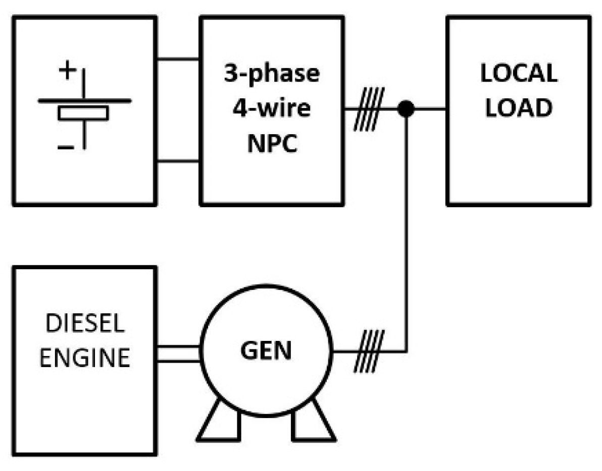
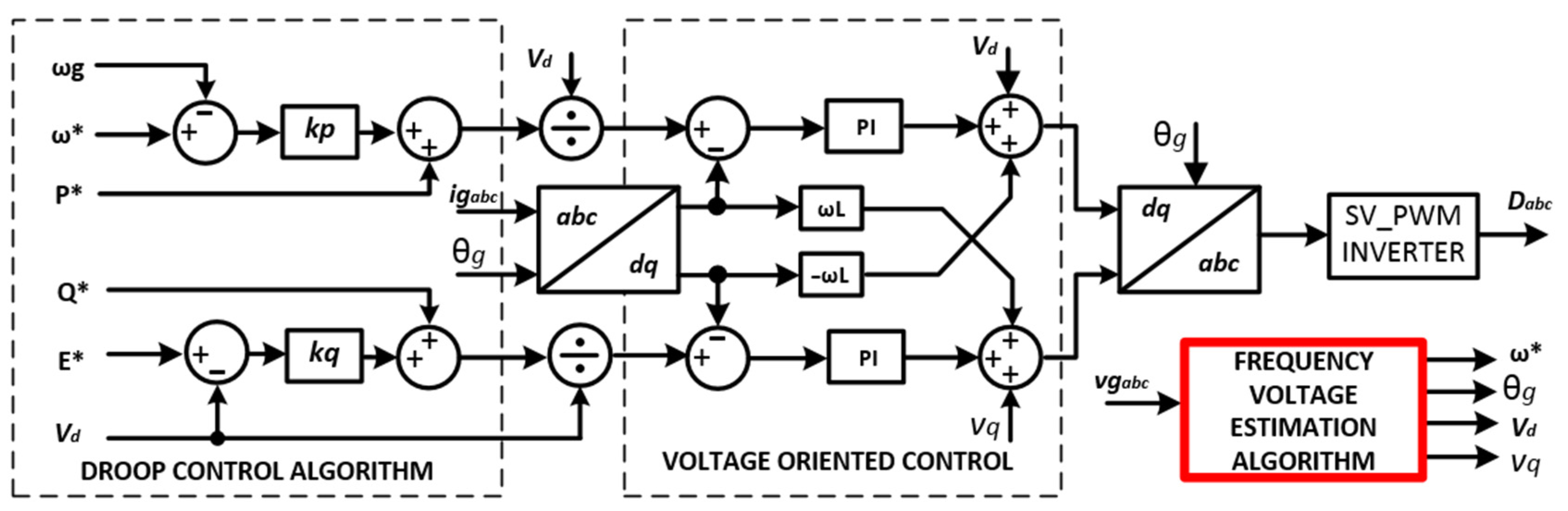
:1. Introduction
2. Frequency Estimation Algorithms
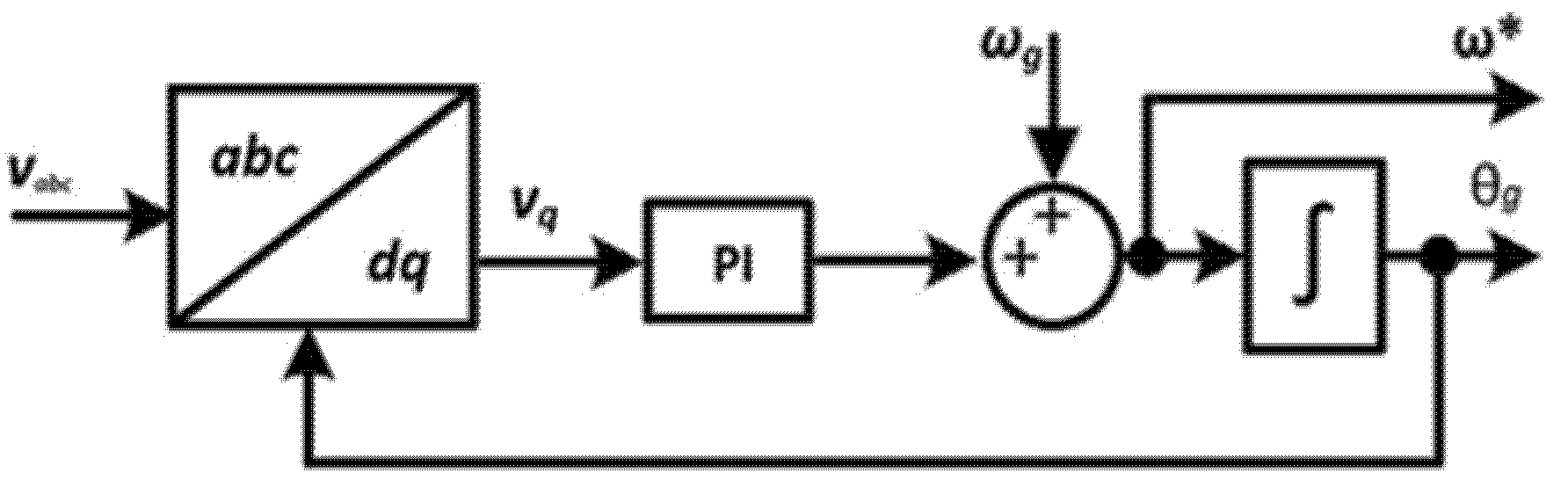
2.1. Synchronous Reference Frame (SRF–PLL)
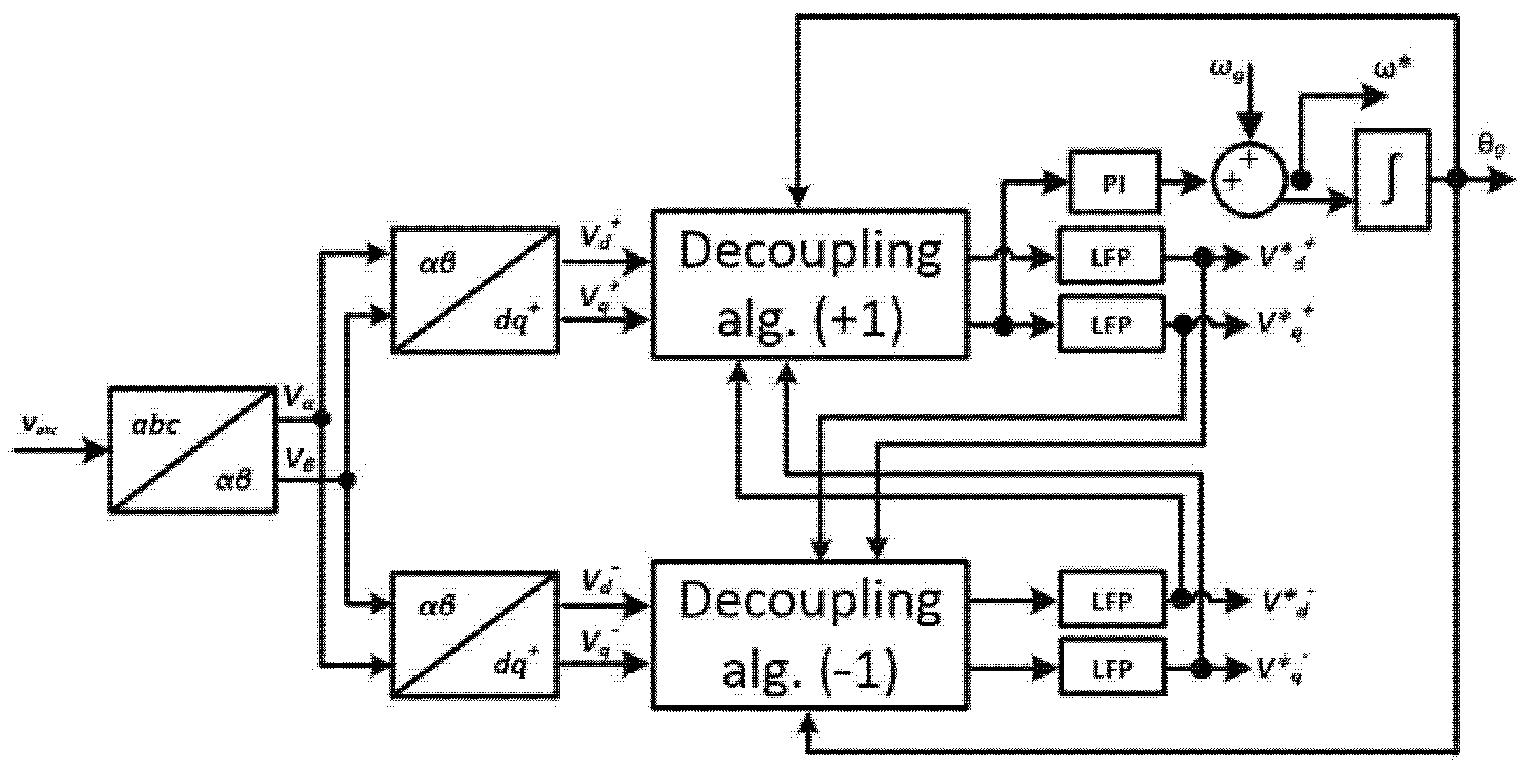
2.2. Double Decoupled Synchronous Reference Frame (DDSRF–FLL)
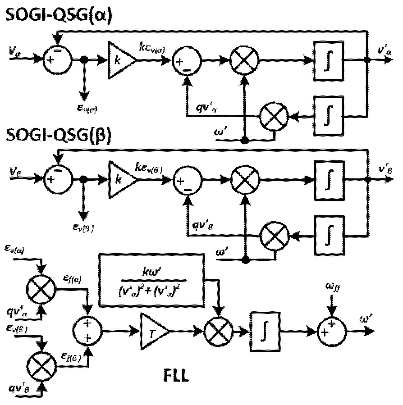
2.3. Double Second Order Generalized Integrator FLL (DSOGI-FLL)
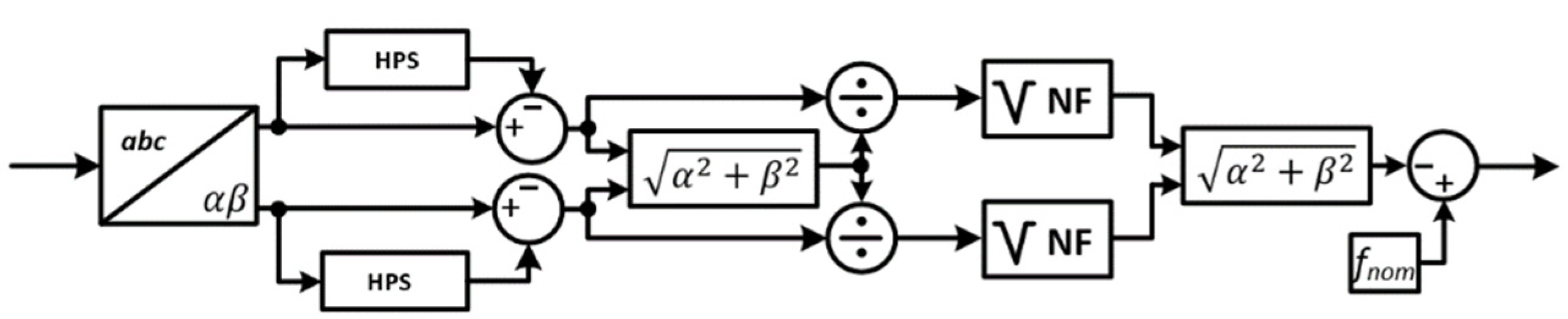
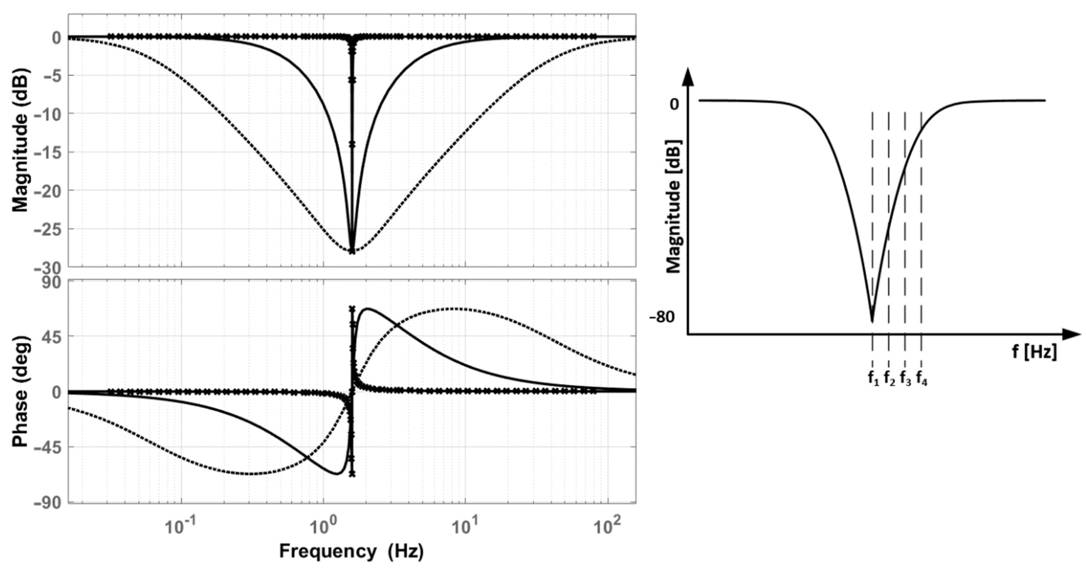
2.4. Resonant Frequency Estimator (RFE)
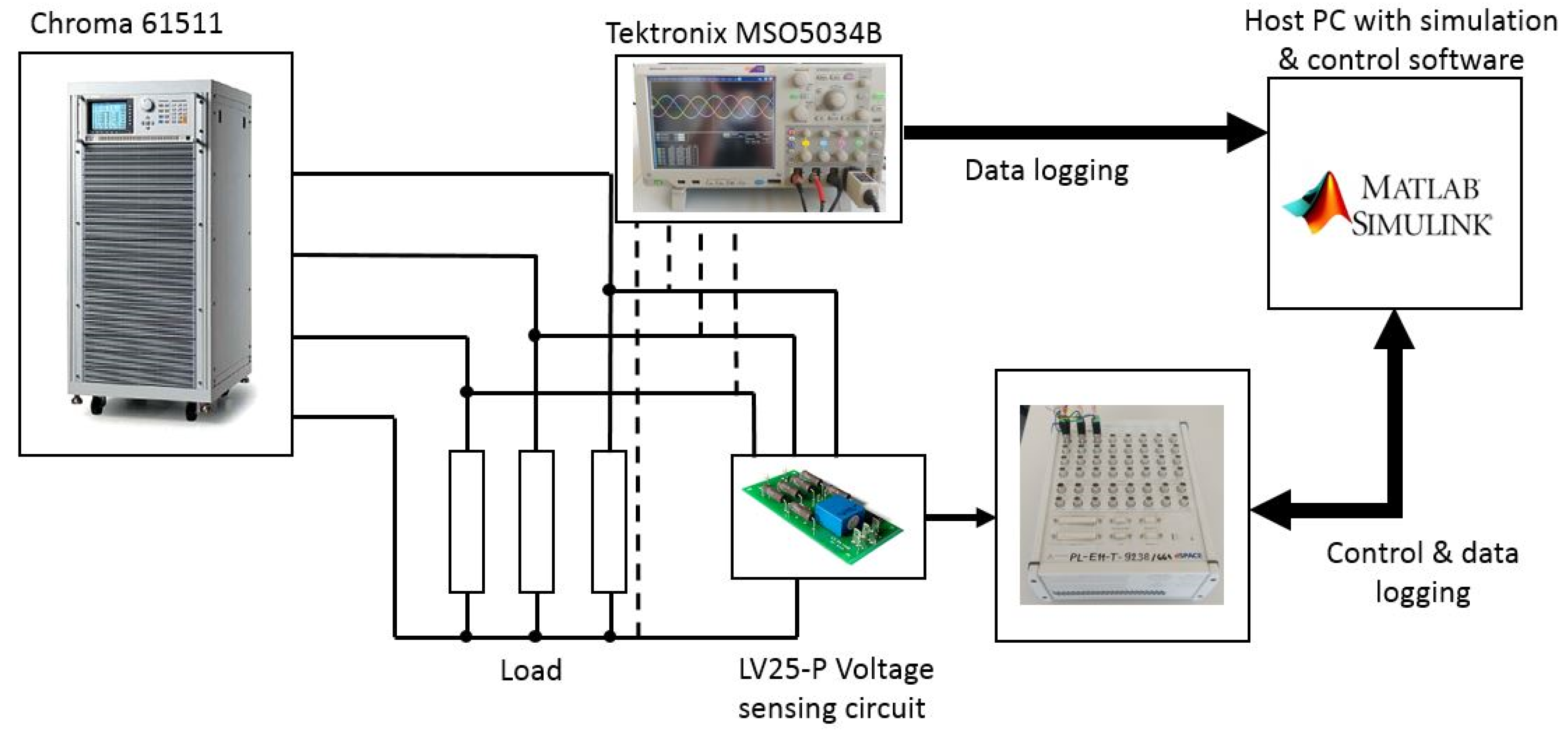
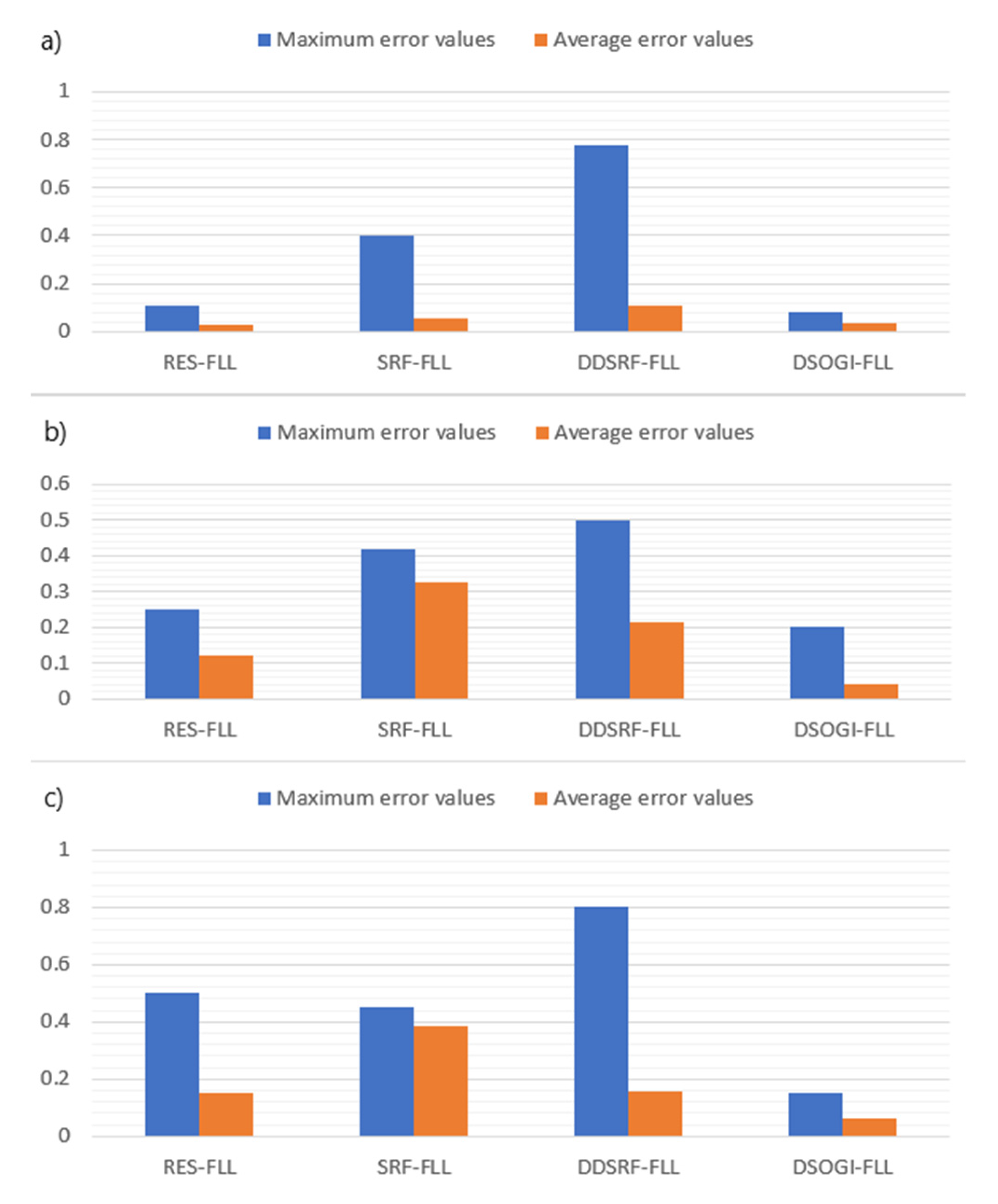
3. Frequency Estimation Testing
- (a)
- 10% frequency swing;
- (b)
- Higher harmonics injection;
- (c)
- Single-phase short circuit.
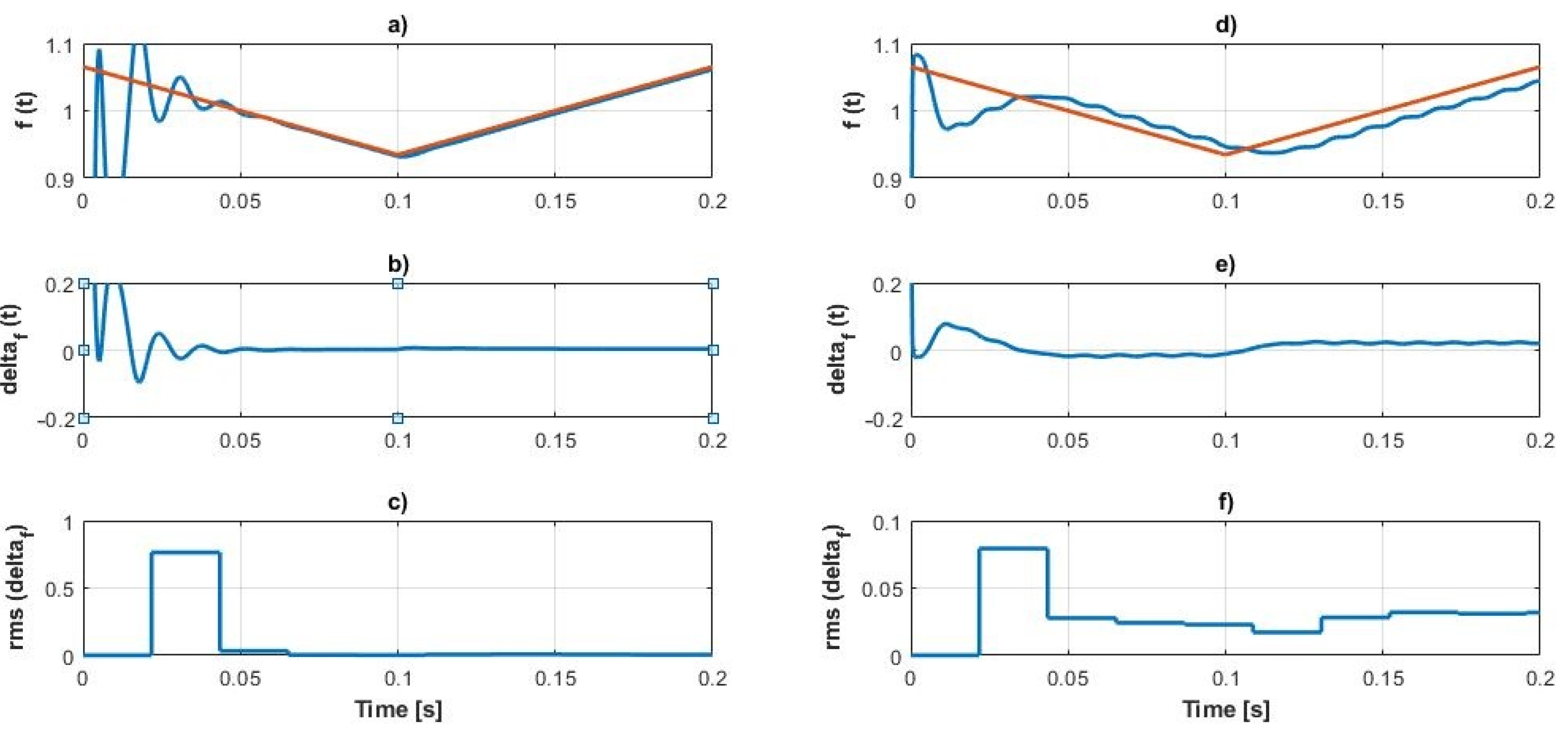
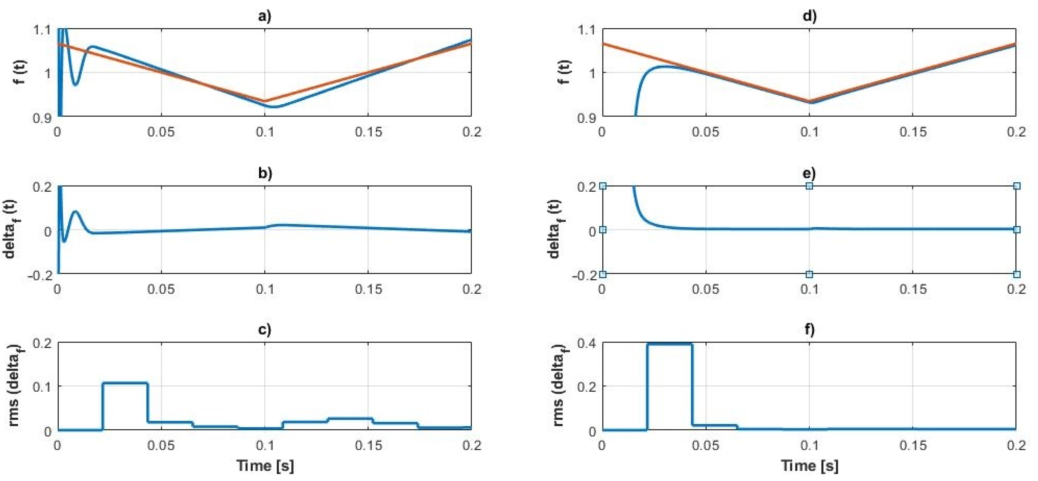
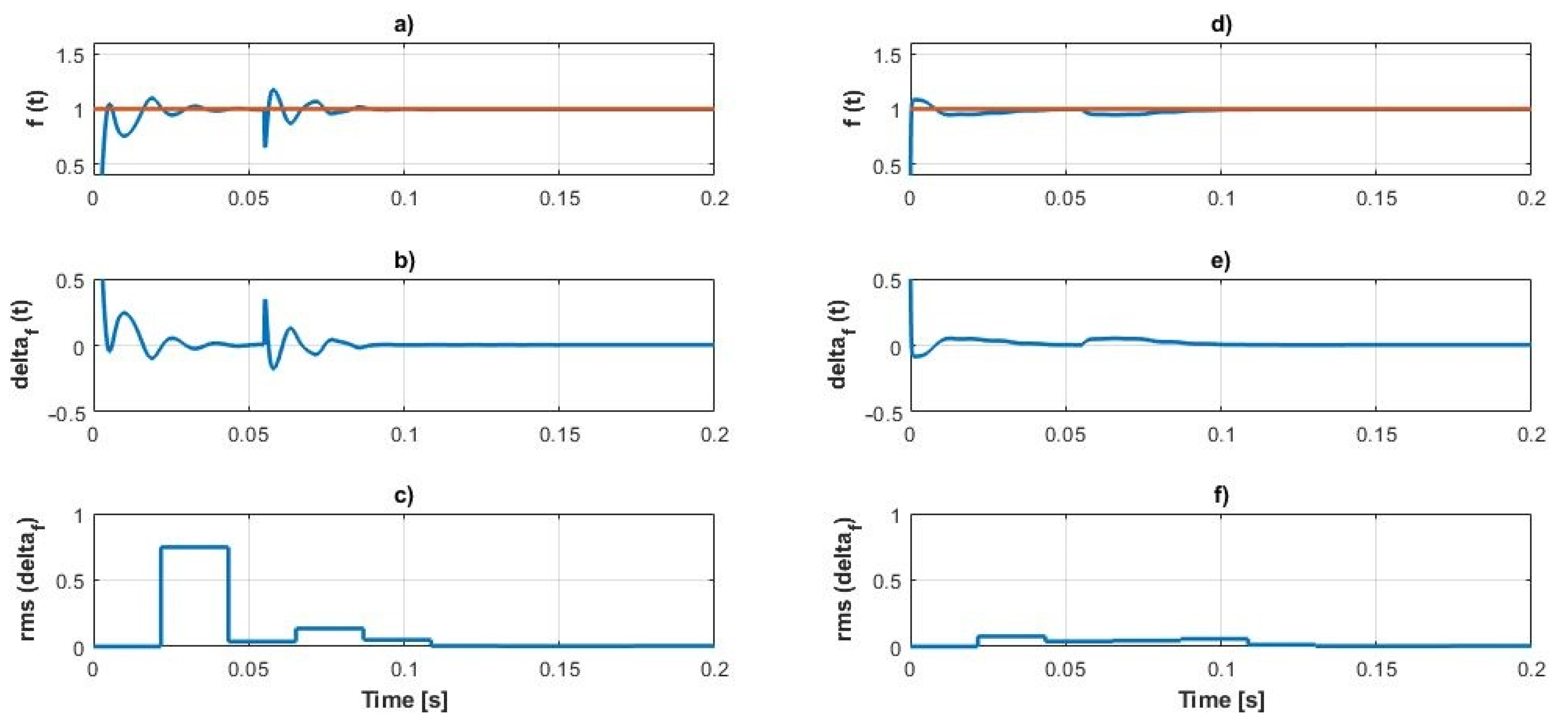
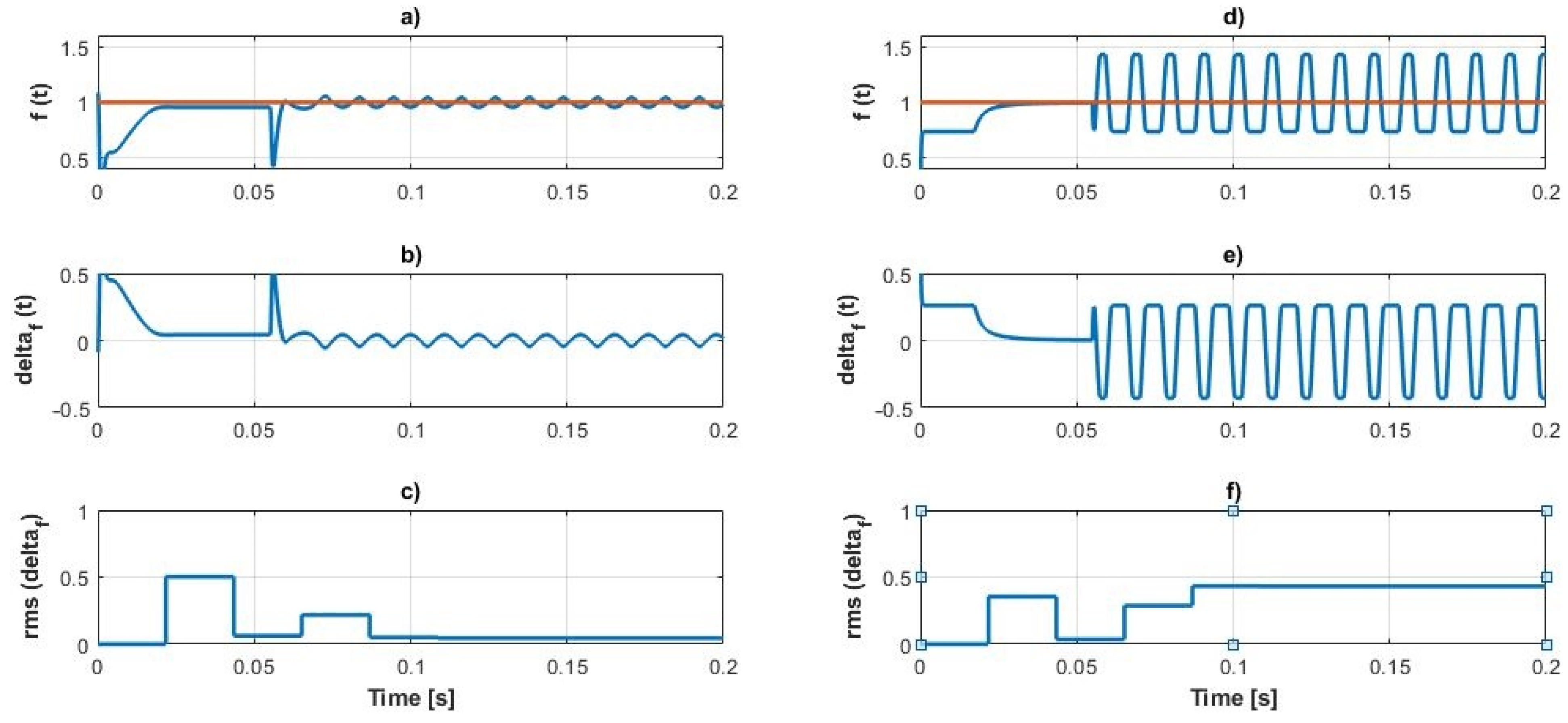
3.1. Frequency Swing
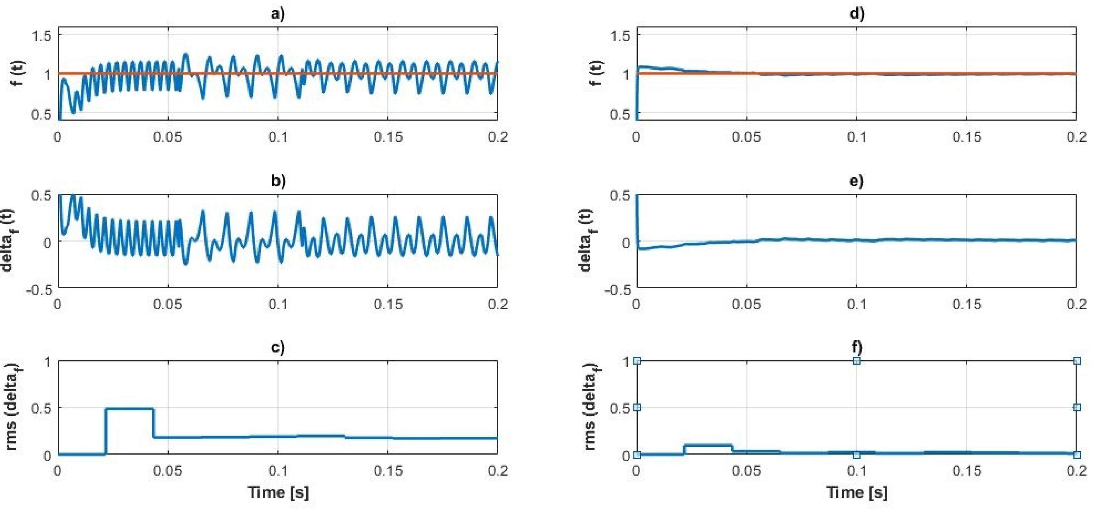
3.2. Harmonics Injection
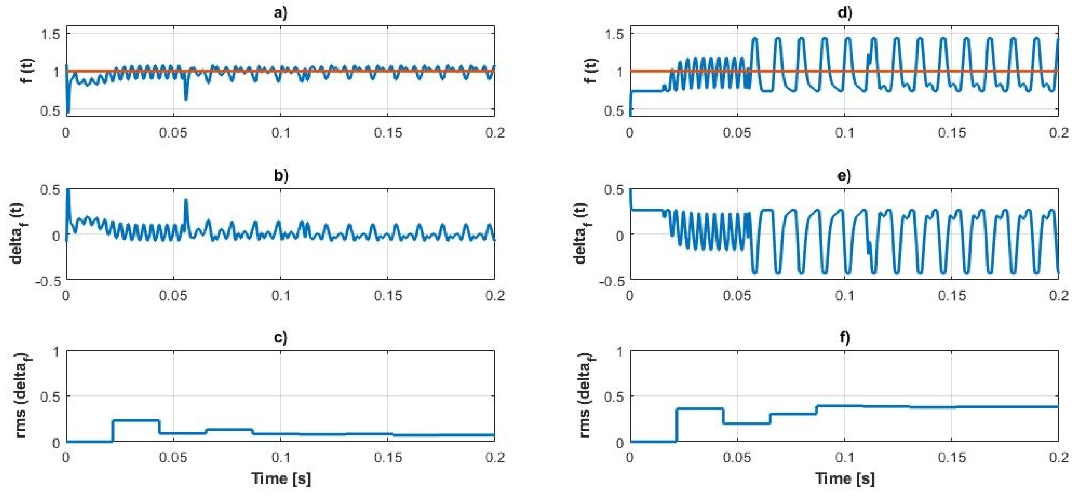
3.3. Asymmetrical Short-Circuit
4. Conclusions
Author Contributions
Funding
Institutional Review Board Statement
Informed Consent Statement
Acknowledgments
Conflicts of Interest
Appendix A. Details of the Test Conditions

| Frequency Swing |
| High frequency: 53 Hz |
| Low frequency: 47 Hz |
| Frequency change rate: ±60 Hz/s |
| Harmonics injection |
| Harmonic frequency: 250 Hz, 350 Hz |
| Total harmonic distortion: 43% of 5th harmonic, 18% of 7th harmonic |
| Asymmetric short-circuit |
| An asymmetric short-circuit was emulated by disconnecting one of voltage measurements from the circuit (resulting in phase voltage readout Vphase = 0 V). |
| SRF-FLL |
| Damping factor ξ = 0.707 |
| Natural frequency ωn = 50 Hz |
| DDSRF-FLL |
| Damping factor ξ = 0.707 |
| Natural frequency ωn = 50 Hz |
| DSOGI-FLL |
| Natural frequency ω = 50 Hz |
| Damping factor k = 0.8 |
| Settling time T = 50 |
| RFE |
| Damping factor ξ1 = 0.001 |
| Damping factor ξ2 = 0.1 |
| Resonant frequency ωn = 42 Hz |
References
- Dragicevic, T.; Alhasheem, M.; Lu, M.; Blaabjerg, F. Improved model predictive control for high voltage quality in microgrid applications. In Proceedings of the Energy Conversion Congress and Exposition (ECCE), Cincinnati, OH, USA, 1–5 October 2017; pp. 4475–4480. [Google Scholar]
- Milczarek, A.; Malinowski, M.; Guerrero, J.M. Reactive power management in islanded microgrid-proportional power sharing in hierarchical droop control. IEEE Trans. Smart Grid 2015, 6, 1631–1638. [Google Scholar] [CrossRef] [Green Version]
- Zhou, J.; Cheng, P.T. A modified Q-V droop control for accurate reactive power sharing in distributed generation microgrid. IEEE Trans. Ind. Appl. 2019, 55, 4100–4109. [Google Scholar] [CrossRef]
- Bałkowiec, T.; Koczara, W.; Moskwa, M. Island operation of a three phase adjustable speed generation system. Int. Trans. Electr. Energy Syst. 2019, 29, e2748. [Google Scholar] [CrossRef]
- Iwański, G.; Bigorajski, Ł.; Koczara, W. Speed control with incremental algorithm of minimum fuel consumption tracking for variable speed diesel generator. Energy Convers. Manag. 2018, 161, 182–192. [Google Scholar] [CrossRef]
- Muljadi, E.; Samaan, N.; Gevorgian, V.; Pasupulati, J. Different factors affecting short circuit behavior of a wind power plant. IEEE Trans. Ind. Appl. 2013, 49, 284–292. [Google Scholar] [CrossRef]
- Labella, A.; Filipovic, F.; Petronijevic, M.; Bonfiglio, A.; Procopio, R. An MPC Approach for Grid-Forming Inverters: Theory and Experiment. Energies 2020, 13, 2270. [Google Scholar] [CrossRef]
- Arul, P.; Ramachandaramurthy; Rajkumar, V.R. Control strategies for a hybrid renewable energy system. Renew. Sustain. Energy Rev. 2015, 42, 597–608. [Google Scholar] [CrossRef]
- Yang, Y.; Blaabjerg, F.; Zou, Z. Benchmarking of grid fault modes in single-phase grid-connected photovoltaic systems. IEEE Trans Ind. Appl. 2013, 49, 2167–2176. [Google Scholar] [CrossRef]
- Luna, A.; Citro, C.; Gavriluta, J.; Hermoso, J.; Candela, I.; Rodriguez, P. Advanced PLL structures for grid synchronization in distributed generation. Renew. Energy Power Qual. J. 2012, 1747–1756. [Google Scholar] [CrossRef]
- Vasquez, J.C.; Guerrero, J.M.; Savaghebi, M.; Eloy-Garcia, J.; Teodorescu, R. Modeling, Analysis and Design of Stationary-Reference Frame Droop-Controlled Parallel Three-Phase Voltage Source Inverters. IEEE Trans. Ind. Electron. 2014, 60, 1271–1280. [Google Scholar] [CrossRef] [Green Version]
- Wen, H.; Guo, S.; Teng, Z.; Li, S.; Yang, Y. Frequency estimation of distorted and noisy signals in power systems by FFT-based approach. IEEE Trans. Power Syst. 2014, 29, 765–774. [Google Scholar] [CrossRef]
- Freijedo, F.; Doval-Gandoy, J.; López, Ó. A Generic Open-Loop Algorithm for Three-Phase Grid Voltage/Current Synchronization With Particular Reference to Phase, Frequency, and Amplitude Estimation. IEEE Trans. Power Electron. 2009, 24, 94–107. [Google Scholar] [CrossRef]
- Xiao, F.; Dong, L.; Xiaozhong, L. A Novel Open-Loop Frequency Estimation Method for Single-Phase Grid Synchronization Under Distorted Conditions. IEEE J. Emerg. Sel. Top. Power Electron. 2017, 5, 1287–1297. [Google Scholar] [CrossRef]
- Xia, Y.; Douglas, S.; Mandic, D. Adaptive Frequency Estimation in Smart Grid Applications: Exploiting Noncircularity and Widely Linear Adaptive Estimators. IEEE Signal Process. Mag. 2012, 29, 44–54. [Google Scholar] [CrossRef] [Green Version]
- Nicastri, A.; Nagliero, A. Comparison and evaluation of the PLL techniques for the design of the grid-connected inverter systems. In Proceedings of the IEEE International Symposium on Industrial Electronics, Bari, Italy, 4–7 July 2010. [Google Scholar]
- Teodorescu, R.; Candela, I.; Liserre, M.; Blaabjerg, F. New Positive-sequence Votlage Detector for Grid Synchronization of Power Converters under Faulty Grid Conditions. In Proceedings of the Power Electronics Specialists Conference, Jeju, Korea, 18–22 June 2006; pp. 1–7. [Google Scholar]
- Blaabjerg, F.; Teodorescu, R.; Liserre, M.; Timbus, A. Overview of control and grid synchronization for distributed power generation systems. IEEE Trans Ind. Electron. 2006, 53, 1398–1409. [Google Scholar] [CrossRef] [Green Version]
- Jaalam, N.; Rahim, N.; Bakar, A.; Tan, C.; Haida, A. Comprehensive review of synchronization methods for grid-connected converters of renewable energy source. Renew. Sustain. Energy Rev. 2016, 59, 1471–1481. [Google Scholar] [CrossRef] [Green Version]
- Guerrero-Rodríguez, N.; Rey-Boué, A.; Bueno, E.; Ortiz, O.; Reyes-Archundia, E. Synchronization algorithms for grid-connected renewable systems. Overview, tests and comparative analysis. Renew. Sustain. Energy Rev. 2017, 75, 629–643. [Google Scholar] [CrossRef]
- Reyes, M.; Rodriguez, P.; Vazquez, S.; Luna, A.; Teodorescu, R.; Carrasco, J. Enhanced decoupled double synchronous reference frame current controller for unbalanced grid-voltage conditions. IEEE Trans Power Electron. 2012, 27, 3934–3943. [Google Scholar] [CrossRef]
- Rodriguez, P.; Pou, J.; Bergas, J.; Candela, J.; Burgos, R.; Boroyevich, D. Decoupled double synchronous reference frame PLL for power converters control. IEEE Trans Power Electron. 2007, 22, 584–592. [Google Scholar] [CrossRef]
- Jarzyna, W.; Zieliński, D.; Gopakumar, K. An evaluation of the accuracy of inverter sync angle during the grid’s disturbances. Metrol. Meas. Syst. 2020, 27, 355–371. [Google Scholar]
- Jarzyna, W. A survey of the synchronization process of synchronous generators and power electronic converters. Bull. Pol. Acad. Sci. 2019, 67, 1069–1083. [Google Scholar]

| SRF-FLL | DDSRF-FLL | DSOGI-FLL | RFE |
|---|---|---|---|
| Frequency swing | |||
|
|
|
|
| Harmonics injection | |||
|
|
|
|
| Asymmetric short-circuit | |||
|
|
|
|
Publisher’s Note: MDPI stays neutral with regard to jurisdictional claims in published maps and institutional affiliations. |
© 2021 by the authors. Licensee MDPI, Basel, Switzerland. This article is an open access article distributed under the terms and conditions of the Creative Commons Attribution (CC BY) license (https://creativecommons.org/licenses/by/4.0/).
Share and Cite
Zieliński, D.; Fatyga, K. Frequency Estimation for Grid-Tied Inverters Using Resonant Frequency Estimator. Energies 2021, 14, 6513. https://doi.org/10.3390/en14206513
Zieliński D, Fatyga K. Frequency Estimation for Grid-Tied Inverters Using Resonant Frequency Estimator. Energies. 2021; 14(20):6513. https://doi.org/10.3390/en14206513
Chicago/Turabian StyleZieliński, Dariusz, and Karol Fatyga. 2021. "Frequency Estimation for Grid-Tied Inverters Using Resonant Frequency Estimator" Energies 14, no. 20: 6513. https://doi.org/10.3390/en14206513
APA StyleZieliński, D., & Fatyga, K. (2021). Frequency Estimation for Grid-Tied Inverters Using Resonant Frequency Estimator. Energies, 14(20), 6513. https://doi.org/10.3390/en14206513