Analysis of the Suitability of Signal Features for Individual Sensor Types in the Diagnosis of Gradual Tool Wear in Turning

Abstract

There are many items in the literature indicating that certain signal features (SFs) of cutting forces, vibrations or acoustic emission are useful for the diagnosis of tool wear in certain single experiments. There is no answer to whether these SFs are universal. The novelty of this article is an attempt to answer these questions and propose a large set of SFs related to tool wear, but without including superfluous SFs. The analysis of the usefulness of the signal properties for the state of the cutting tool in turning was carried out on a large experiment. A number of various SFs obtained for various signal analysis methods were selected for the study. It is found that no SF is always related to the tool wear, so we define many different signal characteristics that can be related to the tool wear (basic set) and automatically select those associated with it in a given machining case. To this end, the relationship between the measures and the wear of the tool was analyzed. Interrelated measures were excluded from it. The obtained results can be used to build a new generation of more effective tool wear diagnostics systems. One of the goals of the tool wear diagnosis system is to save the energy used. The results can also enable the refinement of existing algorithms that predict the energy consumption of a machine.

1. Introduction

The electromechanical industry, including the machining industry [1], is considered one of the main sources responsible for energy consumption. The demand for the energy of machinery centers is determined by design functions, machining processes, energy consumption by auxiliary devices, etc. [2]. In these categories, smaller factors can also be identified, such as the degree of the cutting tool wear. Over the past few years, publications appeared that relate to this issue in the machine tool industry. In the available literature, issues related to identifying appropriate machining strategies [3], planning of machining processes [4] or analyses of new machining methods [5] in the context of energy consumption have been described.

In the paper [6], the impact of the tool wear on the energy consumption of machining processes was analyzed. The presented results showed that an upward trend occurred in energy consumption by the machine tool together with progressive tool wear. In the case of mass production, the development of a solution informing the user about the need to change the tool is very desirable. Tool wear knowledge can be used, for example, in the construction of automatic machine energy monitoring systems [7]. The interest of researchers with the subject of the impact of tool wear on energy consumption also confirms paper [8]. The authors investigate the relationship between the machining speed, tool wear and energy consumption during the machining process.

In the literature, different strategies for minimizing energy consumption can be extracted during machining. They include the selection of optimal process parameters or the development of effective numerical models for machine tools [9]. Strategies aimed at minimizing energy have gained popularity in recent years, and several works refer to energy analysis in various machining processes. Some significant research results on energy modeling and cost reduction and sustainable machining strategies can be found in the following papers [10,11,12].

The study [13] presents a review of literature from the last two decades, dedicated Indirect Tool Condition Monitoring Systems (TCMS). While making a critical analysis of available papers and presenting current trends, the authors concluded that advanced support and monitoring systems of the tools form the way to the development of the machining industry, and as a consequence also to the development of Industry 4.0. This has its justification that one of the overarching goals of TCMS is to optimize parameters such as: tool wear, consumed power and energy, dimensional accuracy, surface quality, manufacturing costs, production time, idle time, amount of waste materials. Therefore, the development of diagnostic systems for machining processes is a very current topic with both scientific and utilitarian significance.

One of the conditions for increasing the autonomy of modern cutting machine tools is the use of a cutting process diagnostic system in them. The issue of tool condition monitoring includes the estimation of gradual tool wear [14], accelerated tool wear detection [15] and catastrophic tool failure detection [16].

The general structure of a tool and cutting process diagnostic system is shown in Figure 1. A number of physical quantities are present in the cutting zone, some of which are correlated with the tool condition. Appropriate sensors convert these quantities into electrical signals, which are subjected to more or less complex processing, starting from filtering, through conversion into digital form, to the determination of SFs useful for diagnostics. Based on the selected SFs, a diagnosis of the tool condition is generated, which can be transmitted to the machine tool control system, which takes appropriate action. Monitoring can be a part of the described structure, from the measurement of physical quantities to the determination of SFs, which can, for example, be displayed as information for the operator. If the tool condition is determined on the basis of the calculated SFs, monitoring becomes diagnostics. On the basis of this tool condition, a command can be worked out, which is automatically transferred to the machine tool control system. Then we are dealing with supervising.

In these systems, the diagnosis of tool wear is usually based on tracking one selected signal feature (usually a mean value) and triggering a tool replacement alarm when it exceeds a threshold value. This value is determined from the value of the SF that it takes when the tool reaches its wear limit, i.e., when the tool is blunted for the first teaching periods of tool life [17,18].

However, commercial diagnostic systems do not currently provide fully satisfactory results [19]. For this reason, many laboratories are still working on improving their diagnostic systems. On the one hand, new features of diagnostic signals are being developed, and on the other hand, new diagnostic methods are being developed as a result.

It is generally acknowledged that reliable process condition monitoring based on a single Signal Feature (SF) is not feasible. Therefore, the calculation of a sufficient number of SFs related to the tool and/or process conditions [20] is a key issue in machining monitoring systems. This is obtained through signal processing methods that comprise the stages shown in Figure 2.

First, pre-processing (filtering, amplification, A/D conversion, segmentation) including, on occasion, signal transformation into frequency or time–frequency domain (Fourier Transform, Wavelet Transform, etc.). The next stage is the extraction of signal features or signal transform features changing with tool or process conditions. There are many diverse descriptors from different sensor signals, but most cannot be easily related to the process being monitored. Thus, SF selection is of critical importance and the identified relevant SFs are finally integrated into the tool or process condition diagnosis system.

In the time domain, statistical features are usually used as features of the signal with the tool state. Where, in addition to the mean or RMS value of the signal, features of the spread of the signal around the mean value such as variance or standard deviation are also used [21,22,23]. There are also publications where, in addition to the above, numerous other statistical features are used [24,25,26,27,28,29,30,31,32,33,34]. The most common are features of the shape and symmetry of the signal distribution (kurtosis and skewness) and values characterizing the size of individual signal deviations (maximum/minimum, crest factor, range or peak-to-peak). However, the latter may result not so much from a change in the state of the tool but, for example, from random mechanical or electrical disturbances, and may therefore be characterized by high randomness.

Although these statistical features characterize many features of a signal, sometimes the nature of a signal cannot be described by simple statistical features. That is why sometimes other features are looked for, e.g., in [35,36] is used Energy entropy. Others, on the other hand, use SFs specific to the type of signal. For example, for cutting force signals, features of the relationship between the cutting force components are proposed [37] or the value of the resultant component of the cutting force [38]. On the other hand, for a raw acoustic emission signal with a specific waveform, very good features are the parameters of exceeding the threshold (of a given value) of the signal [35,36,39] whether [40] (number of occurrences of threshold exceedance and duration of threshold exceedance).

However, methods based solely on the time domain are shown to be insufficiently well correlated with tool wear, hence the need to seek features of the signals undergoing processing. Of these, methods based on frequency domain analysis dominate, of which the Fast Fourier Transform (FFT) is the most commonly used, but there are also more advanced methods, such as Power Spectral Density (PSD) [33]. Various SFs are determined as features of signals in the frequency domain. The most commonly analyzed are the amplitude values of individual frequency bands [22,41,42]. The value of the dominant frequency is often used as an SF [22,27] or the power is determined, or the energy entropy of a given frequency range [27,31]. Sometimes the spectrum of a signal is used as its own signal, and various statistical features are determined for it, such as in [43] where the slant and kurtosis of the signal presented in the frequency domain are determined, or [28] where additionally the mean and variance of the spectrum are determined. In [34] the maximum value, variance and kurtosis of the force signals are determined. In turn, in [33] is the designated mean and standard deviation value of the power spectral density.

However, as numerous studies have shown, the signal during cutting is not stationary—it happens that during stable machining, the signal changes in a non-stationary way, e.g., due to chip breakage, chipping or vibration. As the state of the cutting edge changes, the character of this non-stationarity of the signal can change, therefore all methods that assume the stability of the signal for a specific state of the cutting edge, i.e., based only on the time or frequency domain, may not be sufficient in some situations. That is why it is advisable to use methods based on signal analysis in both time and frequency domains. The simplest of those methods is commonly known as Fast Fourier Transform STFT applied, e.g., in [44]. However, this method has its limitations. Therefore, other methods are being sought. A more advanced method, effectively used to diagnose both natural and catastrophic tool wear, is based on the Hilbert–Huang Transform, used, e.g., in [45,46]. One of the most common methods of time-frequency analysis is the Wavelet Packet Transform (WPT). This method is de facto based on specific filtering of the original signals, which results in a number of band signals (packets). WPT decomposes the signal into the scaling coefficients (approximations A) and the wavelet coefficients (details D) by convolution of the signal and impulse response of the low-pass and high-pass filters. The filter’s outputs are subsampled by 2. At the first level, the original signal is decomposed into A and D packets, then approximation A can be decomposed again into AA and AD and detail can be decomposed again into DA and DD packets. The range of the level of these bands depends on the sampling frequency and the level. A three-level WPT decomposition tree is presented in Figure 3. The principle of the Wavelet Packet Transform is described, e.g., in [36].

Since, in contrast to a signal in the frequency domain represented as a spectrum, the result of the WPT resembles a series of time waveforms, similar SFs as for signals in the time domain are usually used as SFs of individual packets (bandpass signals). Most often RMS is used as the only feature [29,47,48]. However, some publications also use other statistical features like standard deviation [22,27,32] kurtosis [35,36], skewness [35,36], peak-to-peak value [32], crest factor [27] and others [49]. A popular SF used in many publications as a feature of packages is Energy entropy. For example, in [50] Energy entropy is used as an SF of vibration signals during longitudinal turning; in [27,35] is used as SF of force and modulated acoustic emission signal during face turning, in [36] is used as SF of raw acoustic emission signal during face turning.

In some works, several methods of signal analysis are used simultaneously, e.g.:

• in the time and frequency domain: e.g., time domain and FFT spectrum was used to SFs calculation for tool condition monitoring during milling [28,34], turning [31] and drilling [51]; in [33] time domain and PSD spectrum was used to SFs calculation during milling;
• in the time domain and time–frequency domain; e.g., time domain and Wavelet Packet was used to SFs calculation in turning [30,35] and milling [32]; in the time, frequency and time–frequency domain [22,27].

In summary, in many publications, it is shown that many different signal features (of cutting forces, vibrations or acoustic emission) obtained by different signal processing methods are useful for the diagnosis of tool wear. However, in each of these publications, the authors usually present only a small number of SFs tested for individual experimental studies. They lack the answer to whether and to what extent these SFs are universal, which features always carry the same practical information, i.e., which are redundant. The novelty of this article is to try to answer these questions and to propose a large set of SFs that may be related to the tool wear, but not including redundant features.

In the literature, the choice of SFs used is made manually by the researcher, usually without justification for the choice. This approach is only possible in a laboratory setting, where the scientist can, for example, make a selection of features based on the nature of the signal obtained. In industrial reality, it is not possible for an operator or technologist to decide on the choice of features for specific processing conditions. Thus, one has to arbitrarily make the choice of features at the design stage of the industrial system. It is therefore possible to select a large number of gauges with the assumption that one of them will be sufficiently useful from the point of view of diagnostics of the tool condition. However, by using a large number of gauges there is a risk of generating a large number of gauges that are completely uncorrelated with the condition of the tool, do not carry any information in the particular case, so they interfere with the operation of the system, or even make the indications completely wrong. Too many SFs also affect the calculation time and potentially overload the system with too many calculations and data. On the other hand, cautious use of too few SFs carries the risk of not using the information potential of the signal and, consequently, also less accurate indications of the system.

When building a supervisory system, one should select in advance SFs that have a high probability of being useful in diagnostic systems, i.e., they have a chance of being correlated with the state of a tool, but also have a chance of being original SFs, not correlated with other SFs, i.e., bringing new information. There are hundreds of possible SFs, testing the usefulness of all of them is computationally expensive, so it is worth making a general initial selection, i.e., selecting SFs that may (but do not have to) be potentially valuable. When selecting SFs, the way of further diagnostics and the resulting model of dependence of a given signal feature on the state of the tool are important. The simplest model assumes a monotonic increase in the feature with the progress of the tool wear. However, as reality shows, such an assumption is very simplified. It does not assume, e.g., decreasing, or non-monotonic changes of SFs, which greatly limits the accuracy of its indications. Therefore, many laboratories are currently working on algorithms for diagnosing tool wear based on more complex models of dependence of SFs on the condition of the tool. This model is not generic but is built for each new machining case on the basis of learning data. As with commercial systems, these data are taken from one or more of the first periods of tool life performed under operator supervision. Neural networks have been used as a model for a very long time, most commonly a multilayer perceptron [52]. Newer more effective solutions are now being used as a model. For example, in [14] applied ensemble learning (EL) classifier to establish a nonlinear mapping relationship between the SFs and the tool wear level, in [53] which is then modelled by a recurrent neural network, capturing the evolutive pattern of wear over time, in [54] stacked sparse autoencoder neural network was used to monitor the tool wear state.

Each of these models is built on a selected set of SFs. In most work in the field of tool condition diagnostics, the SFs are still chosen arbitrarily [55]. Depending on the machine tool, tool or workpiece material used, different SFs are best evaluated. For example, it was shown that for coated tools, the average values of the feed and feed-rate components of the cutting force are SFs of cutting forces that can act as wear symptoms, while for uncoated tools the standard deviations of all three components of the cutting force can act as wear symptoms [56]. In [57] using linear discriminant analysis to select the SFs, it was shown that for different workpiece materials, different SFs related to the condition of the tool were obtained. The need to apply a data selection algorithm to a diagnostic system was recognized as early as the mid-1990s [58]. A popular solution to this problem is to determine the Pearson linear correlation coefficient between a single SF and tool wear [59]; however, this coefficient tells whether an SF is related to tool wear according to a linear relationship. An SF that is very closely related to tool wear according to a non-linear relationship gets a low score, which is an inadequacy of the Pearson coefficient for the assessment of SFs. A better solution is to use Spearman’s rank correlation coefficient [60]. However, even this is a coefficient that only tells whether there is a monotonic relationship between the SF and tool wear. Attempts have also been made to use more universal indicators that could recognize a relationship of any form, such as the coefficient of determination [61]. Discriminant analysis and the associated Fischer linear discriminator (FDA) were also used to select SFs [62]. Other methods of assessing SFs such as linear regression were also used [63] whether Taguchi’s method of orthogonal arrays [64].

The SFs selection methods discussed above do not consider the subsequent integration of SFs. It is by no means obvious that the best SFs for a given integration method will turn out to be equally beneficial for another one, or that a given feature selection method is at all suitable for a given feature integration method. Instead, it is obvious that the best set of SFs for a given integration model is the set on which the model achieves the best diagnostic results. Thus, the best criterion for the evaluation of a feature is its influence on the accuracy of the tool state estimation. An example of this type of solution can be the pruning of FFBP neural network weights described in [65].

In this article, the authors determine the usefulness of a feature for diagnosing tool wear based on the accuracy of estimating tool wear on a given feature. The research was carried out for four different turning operations thus selecting SFs characterized by high efficiency and universality.

2. Tests of the Usefulness of Diagnostic Signal Features

2.1. Experimental Setup

It was decided to analyze the usefulness of signal features for tool condition diagnostics during turning using experiments representing the widest possible variety of machining variations and conditions. The description of the experiments is presented in

Table 1. Cutting conditions of experiment.

	Exp 1	Exp 2	Exp 3	Exp 4
Machine type	Lathe VENUS 450	Lathe FAMOT 50	Lathe TKX 50N	Lathe TKX 50N
cooling	NO	YES	YES	YES
Workpiece material	1.0503	1.2063	Inconel 625	1.2063
Tool holder	PCLNR 3225P 12	DCLNL-22045-12	CRSNL 3225P12	L 114.16
Tool insert	CNMG 120408	CNMG 120408	RNGN 120700T01020	TNMM 220412
ap [mm]	1.5/2	1	2.5	1
f [mm/rev]	0.1	0.1	0.2	0.1/0.15
vc [m/min]	150	280	220	120
Cutting force sensor	Kistler 9601A31		Kistler 9017B	Kistler 9601 A31
Cutting forces signals	Fx, Fy, Fz	Fx, Fy, Fz	Fx, Fz	Fx, Fy, Fz
AE sensor	Kistler 8152 B121	Kistler 8152B	Kistler 8152 B1	Kistler 8152 B121
AE signals	AErms	AErms	AErms	AErms
Vibration sensor	-	PCB PIEZOTRONICS 356A16	PCB PIEZOTRONICS 356A16	-
Vibrations signals	-	Vx, Vy, Vz,	Vy, Vz	-
Sound sensor	-	MIC-01;SENNHEISER E825S	-	-
Sound signals	-	C1, C2	-	-
Total No. of tool lives	9	5	7	4

Note: C1—electret microphone, C2—dynamic microphone.

and Figure 4.

2.2. Signal Processing

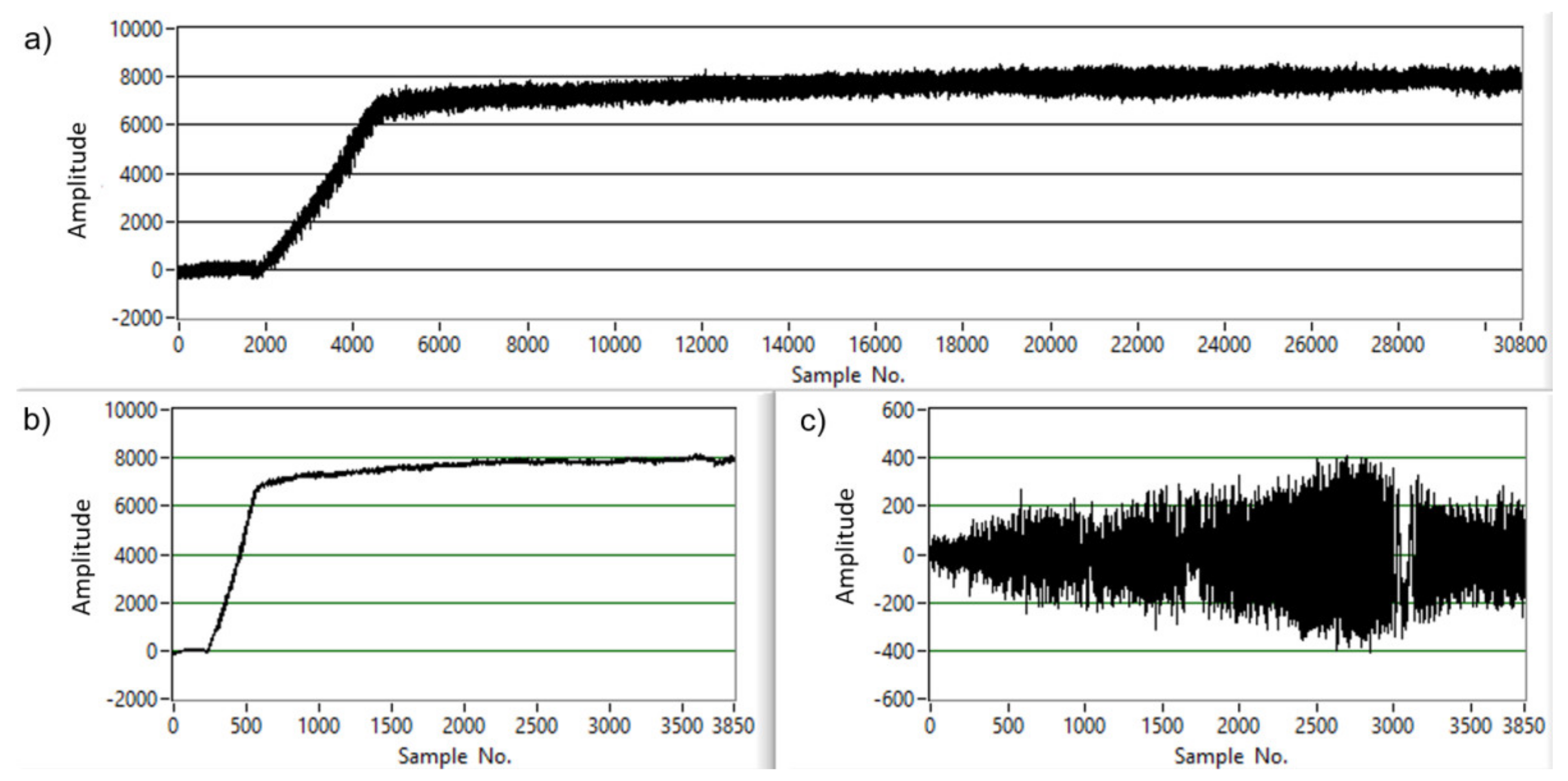
2.2.1. Preprocessing—Signal Segmentation

Before the signal features can be determined, the relevant parts of the original signal, hereafter called segments, must be selected. Suitable signal fragments are those originating from the cutting operation (without run-up, coasting, input and output) and as constant as possible, undisturbed by, e.g., depth changes. The selection of segments is usually performed manually by a researcher (laboratory work) or a machine tool operator, which is difficult, unique and requires a lot of experience. In the Department of Automation and Metal Cutting at Warsaw University of Technology, an algorithm was developed for the automatic selection of segments from stable machining fragments well suited for tool condition diagnostics. A detailed description of the segment selection procedure is described in [66]. Each segment represented a separate diagnostic signal, subjected to determination and SFs.

2.2.2. Feature Extraction

Using previous experience and building on the information described in Section 2.1, it was decided to determine signal features in the time, frequency, and time–frequency domains for each experiment. The general description of signal features used in this research for particular types of signals is presented in

Table 2. General description of signal features.

Equation/ Description of SF	Used for Signal/WP Packet Type
	F			V, C		AErms
	Raw Signal	Packets A, AA, AAA	Packets not A, AA, AAA	Raw Signal	All WP Packet	Raw Signal	All WP Packet
$\overline{x}=\frac{{\displaystyle {{\displaystyle \sum }}_{i=1}^n}{x}_i}{n}$	X	X	-	-	-	X	X
$rms=\sqrt{\frac{{\displaystyle {{\displaystyle \sum }}_{i=1}^n}{x}_i^2}{n}}$	X	X	X	X	X	X	X
$\sigma =\sqrt{\frac{{\displaystyle \sum }_{i=1}^n{\left(x_i-\overline{x}\right)}^2}{n-1}}$	X	X	-	-	-	X	-
$v={\sigma }^2$	X	X	X	X	X	X	X
${\mu }^3=\frac{1}{n}{\displaystyle {\displaystyle \sum }_{i=1}^n}{\left(x_i-\overline{x}\right)}^3$	X	X	X	X	X	X	X
${\mu }^4=\frac{1}{n}{\displaystyle {\displaystyle \sum }_{i=1}^n}{\left(x_i-\overline{x}\right)}^4$	X	X	X	X	X	X	X
$Sk=\frac{{\mu }^3}{{\sigma }^3}$	X	X	X	X	X	X	X
$K=\frac{{\mu }^4}{{\sigma }^4}$	X	X	X	X	X	X	X
$P=\frac{1}{n}{\displaystyle {\displaystyle \sum }_{i=1}^n}{x}^2$	X	X	X	X	X	X	X
$PP=max-min$	X	X	X	X	X	X	X
$CF=\frac{max}{rms}$	X	X	X	X	X	X	X
Perc90: Signal value below which 90% of samples were	X	X	X	X	X	X	X
Perc50: Signal value below which 50% of samples were	X	X	-	-	-	X	X
$E=\frac{{{\displaystyle \sum }}_{i=1}^n\log x_i^2}{n}$	X	X	X	X	X	X	X
$Shan=\frac{{{\displaystyle \sum }}_{i=1}^n{x}_i^2\log x_i^2}{n}$	X	X	X	X	X	X	X
$Incr=\frac{rm{s}_k-rm{s}_1}{rm{s}_1}$	X	X	X	X	X	X	X
Count1: for threshold = 30% max1	-	-	X	X	X	X	X
Count2: for threshold = 50% max1	-	-	X	X	X	X	X
Count3: for threshold = 70% max1	-	-	X	X	X	X	X
Pulse1: for threshold =30% max1	-	-	X	X	X	X	X
Pulse2: for threshold = 50% max1	-	-	X	X	X	X	X
Pulse3: for threshold = 70% max1	-	-	X	X	X	X	X
$E=\frac{{{\displaystyle \sum }}_{k=1}^m\log x_k^2}{m}$	X	-	-	X	-	X	-
	X	-	-	X	-	X	-
$F_1=\frac{F_f}{F_c}$	X	-	-	-	-	-
$F_2=\frac{F_p}{F_c}$	X	-	-	-	-	-
$F_3=\frac{F_c}{\sqrt{F_f^2+F_p^2}}$	X/-	-	-	-	-	-
SUMMARY	21/20	16	19	21	19	24	21

*—determined when there are three components of cutting forces.

. The number of segments per single operation for each experiment is shown in

Table 3. General number of SFs for particular experiments.

Title	Exp No 1	Exp No 2	Exp No 3	Exp No 4
Signals Type	Fx, Fy, Fz, AErms	Fx, Fy, Fz, AErms,Vx, Vy, Vz, C1, C2	Fx, Fz,AErms, Vy, Vz	Fx, Fy, Fz, AErms
No. of segments	5	4	4	3
No. of SFs per segment	1146	2581	1444	1146
General No. of SFs	5730	10,324	5776	3438

.

Time Domain

From the time domain, i.e., from the raw, unprocessed signal, it was decided to determine the number of statistical features: RMS, standard deviation (σ), variance (v), mean value ($\overline{x}$), skewness (Sk), kurtosis (K), third-degree moment (μ3), fourth-degree moment (μ4), power (P), peak-to-peak value (PP), crest factor (CF), percentile 90% (Perc90), percentile 50% (Perc50). It was also decided to use the Energy entropy feature (E), Shannon entropy (Shan) and the incremental value Incr (Table 2).

It was decided to use the number of times the three set thresholds were crossed (Count1, Count2, Count3) and the percentages of time over the three thresholds (Pulse1, Pulse2, Pulse3) as a feature. The individual thresholds: 1, 2, and 3 were set as 30%, 50%, 70%, respectively, of the signal’s maximum value during the first operation and were determined from previous studies to be uncorrelated with each other.

Energy entropy deserves special attention here, which, in contrast to variance (or its derivatives, such as standard deviation), is a feature of dispersion that is not very sensitive to individual disturbances. Figure 5 shows a simulation of different signals and the Energy entropy values and variances of these signals. The first graph shows two waveforms—purple and dark blue. The order of magnitude of both signals is similar, but the dark blue waveform contains single pulses. Below the chart, the values of variance are presented (σ ²) and Entropy energy features (E) for both runs. The results show a strong variance response to single signal perturbations, while the energy value remains unchanged. In graph two, the purple waveform has values an order of magnitude higher than in graph one, while the values of the dark blue waveform remain unchanged. The variance value, in this case, showed no difference, while the Energy entropy shows a difference between the two. The difference is due to the logarithm function, which highlights changes by an order of magnitude. In Figure 5 the signal samples in both runs, apart from a few disturbances, have a similar order of magnitude hence the Energy entropy value is similar. In comparison, the variance shows high sensitivity to single perturbations which translates into a significant value of this feature. In Figure 5, both presented signals significantly differ as for the order of magnitude of signal samples, which immediately influences the value of entropy energy. The variance, in this case, shows no difference between signals of such different nature.

Frequency Domain

FFT and PSD were performed as part of the frequency domain analysis. Looking at the obtained spectra for new and blunted tools for different signals, it was observed that it is not possible to isolate specific single frequency bands for which a change of signal value occurs—usually, this change of signal spectrum value occurs in several or more frequency bands, different depending on the experiment analyzed. On the other hand, analysis of the change of the signal value for all individual bars of the spectrum would be equivalent to the determination of the RMS value of wavelet packets obtained as a result of WPT. Therefore, in contrast to commonly used SFs of the spectrum obtained as a result of FFT or PSD, it was decided to use Energy entropy of FFT or PSD spectrum as a feature in the frequency domain. In this case, a single spectrum bar was treated as a single signal sample.

Time–Frequency Domain

To determine SFs in the time–frequency domain, it was decided to apply the WP3 three-level packet wavelet transform using the db02 wavelet. As a result of the transform, 14 packets (band signals) were obtained. According to the scheme presented in Figure 3, if etc. the raw signal contains information about frequencies 0–1000 Hz, two band signals are obtained as a result of the decomposition at the first level: Approximation A (containing information about frequencies 0–500 Hz) and Detail D (containing information about frequencies 500–1000 Hz). At the second level, we obtain four band signals, with a frequency bandwidth of 250 Hz and at the third level, we obtain eight band signals with a frequency bandwidth of 125 Hz. Thus, for each of the diagnostic signals we receive a total of 14 band signals in addition to the raw signal.

For each of the band signals, similar SFs were determined as for the raw signal in the time domain; however, some distinction was made due to the nature of the signal. Thus—for signals oscillating around zero (raw signals and wavelets for vibrations V and sound pressure C, wavelets other than A, AA, AAA for the signal of forces F), it does not make sense to determine the values characterizing the average value of the signal, such as the arithmetic mean or median. On the other hand, for signals containing a constant component (raw signal F, wavelet packets A, AA, AAA for signal F), it does not make sense to determine values exceeding a given threshold. A certain, worldly incongruity from this rule was applied for signal AE_rms. This signal has a non-zero mean value but its value in comparison with the number of pulses increasing with wear is by the order of magnitude smaller due to the short duration of these pulses. Hence, the determination of the threshold exceedance value seems to make as much sense as possible. Therefore, for the AE_rms. signal it was decided to use all features both for signals with non-zero mean value and those characteristics for signals oscillating around zero. The character of particular signals and packages obtained as a result of WPT on the example of machining forces is presented in Figure 6. The original signal (Figure 6a) contains all frequency components—constant components, low-frequency components and high components. The constant component starts from 0, then slowly rises to a certain level. Around constant components, high frequency oscillates high-frequency components. The AAA package (Figure 6b) contains the constant component and some low-frequency components. Here, a level of force signal can be observed. The DDD package contains only the highest frequencies.

The general number of SFs obtained for each study is shown in Table 3.

2.3. Testing the Suitability of Gauges for Tool Condition Diagnostics

Studies on the Correlation of Signal Features with Tool Wear

As a result of signal analysis, many (several hundred) SFs are obtained for each segment of the individual diagnostic signals. Out of all these SFs, it is necessary to select those that are useful for tool condition diagnostics. The suitability of a particular feature for use in a given tool wear diagnosis system is determined by two factors: firstly, the feature must contain information about the condition of the tool and secondly, the diagnosis algorithm must be able to extract this information. Therefore, the feature selection system must consider the capabilities of the wear estimation algorithm based on the given feature.

Therefore, to begin with, we will briefly present the consumption estimation algorithm that was developed for many years at the Department of Automation and Metal Cutting at Warsaw University of Technology (a detailed description of this algorithm can be found in [67]). This algorithm belongs to the group of tool wear estimation methods discussed in the literature review based on building a model of the dependence of diagnostic signal features on learning data.

Tool wear indicator used by the algorithm is the proportion of tool life used, expressed as a % ΔT. It complements the recently 100% popular RUL (remaining useful life) indicator, i.e., the remaining useful life of the tool. The procedure for wear diagnosis is as follows: we determine the feature models based on the first period of tool life; in the second period of tool life, authors estimate the wear on the basis of the measurement models determined after the first period of tool life, then we determine the model based on the first and second period of tool life; in the third period of tool life, authors proceed in a similar way as in the case of the second period, teaching the system. From the fourth period of tool life, the diagnosis is carried out on the basis of models built on the basis of the first three periods of tool life. The error RMSE of the condition diagnosis carried out in this way is denoted as RMSE(T).

The course of the successive (j-th) selected signal features SF of the first “teaching” durations is recorded in the table SF_j [ΔT]. This array is created from courses of feature approximated by a third-degree polynomial. Subsequent index values of the array correspond to the value of ΔT equal to 1%. Based on the table thus determined, the tool wear of successive tools is estimated. In the table SF_j [ΔT] the closest element, whose value is closest to the current value, is searched for SF_j for the tool to be diagnosed. The index of this element specifies the used part of the lifetime in %. The search is limited to the area of the array surrounding the point that corresponds to the wear increment expected from the length of the learning periods of the tool life and the tool wear estimated by the system in the previous step. The boundaries of this area correspond, respectively, to a twice slower and twice faster wear increment than the average of the learning periods. The final value of wear estimated by the system is the average of the estimates for the individual SFs with the rejection of coarse errors, i.e., exceeding 3σ. The effectiveness of such a diagnostic system is determined by the mean square error, calculated according to Equation (1):

$$RMSE=\frac{{{\displaystyle \sum }}_{l=1}^L\sqrt{\frac{{{\displaystyle \sum }}_{k=1}^K{\left(T_{calc,l,k-}{T}_{real,l,k}\right)}^2}{K\left(l\right)}}}{L}$$

(1)

where:

T_calc,l,k—value of the estimated tool wear for the k-th operation of l-th tool life;

T_real,l,k—value of the actual tool wear of the k-th operation l-th lifetime of the tool;

L—number of tool life periods used for teaching;

K(l)—number of operations in l-th tool lifetime.

In order to determine whether a given feature is useful in the above-mentioned method of diagnostics of a tool condition, it is necessary to determine the effectiveness of the system (RMSE error) in the case of learning on a given feature. In the case of testing the effectiveness of a tool wear diagnostic algorithm, the experimental data should be divided into a learning set (used to build the model) and a testing set used to evaluate the effectiveness of the diagnostic algorithm. In order to exclude the influence of random uniqueness of the course of the feature in a single period of tool life, the testing of the system should be repeated many times using all possible combinations of dividing the data into a learning set and a testing set. Here, however, we do not want to test the effectiveness of the diagnostic algorithm but only the suitability of the feature for use by the algorithm. Taking advantage of the fact that in the case of this feature integration algorithm the generalization ability of the model is not adjusted in the learning process to determine the suitability of a given feature for estimation ΔT, A model of the feature was first determined using all the tool life periods and then the diagnostics were carried out on all the tool life periods using this model. The value of the estimation error thus obtained ΔT of the tool is denoted as RMSE(L) and forms the basis for the evaluation of the feature. The more useful a feature is for diagnosis, the more useful the estimation error ΔT_calc in relation to ΔT_real the actual one is smaller.

3. Results and Discussion

3.1. Analysis of the Usefulness of SFs for Tool Condition Diagnostics

In Figure 7, example courses of SFs for individual experiments are presented. The curves are presented as a function of the used part of the tool life (ΔT [%]) for successive shelf-lives—each marked with a different color. The name of the feature, the value of RMSE(L) and the number of the segment for which the feature was determined are shown above each course of the feature.

Looking at these sample SFs only, we can see that:

• For each sensor, SFs correlated with the state of the tool can be extracted;
• The dependence of the signal features, which are correlated with the tool state, can have not only a commonly used monotonic distribution (see Figure 7g), but may also be exponential (see Figure 7d) or show a downward trend (see Figure 7j);
• The same feature for the same type of sensor may show a different pattern for different experiments (see Figure 7a,j);
• The same feature for different sensors of the same physical quantity for the same experiment may take on different values (see Figure 7e);
• For cutting force signals, for wavelet packets not containing a constant component, SFs characteristic of signals oscillating around zero are suitable, e.g., SFs for counting the number of threshold crossings (see Figure 7h);
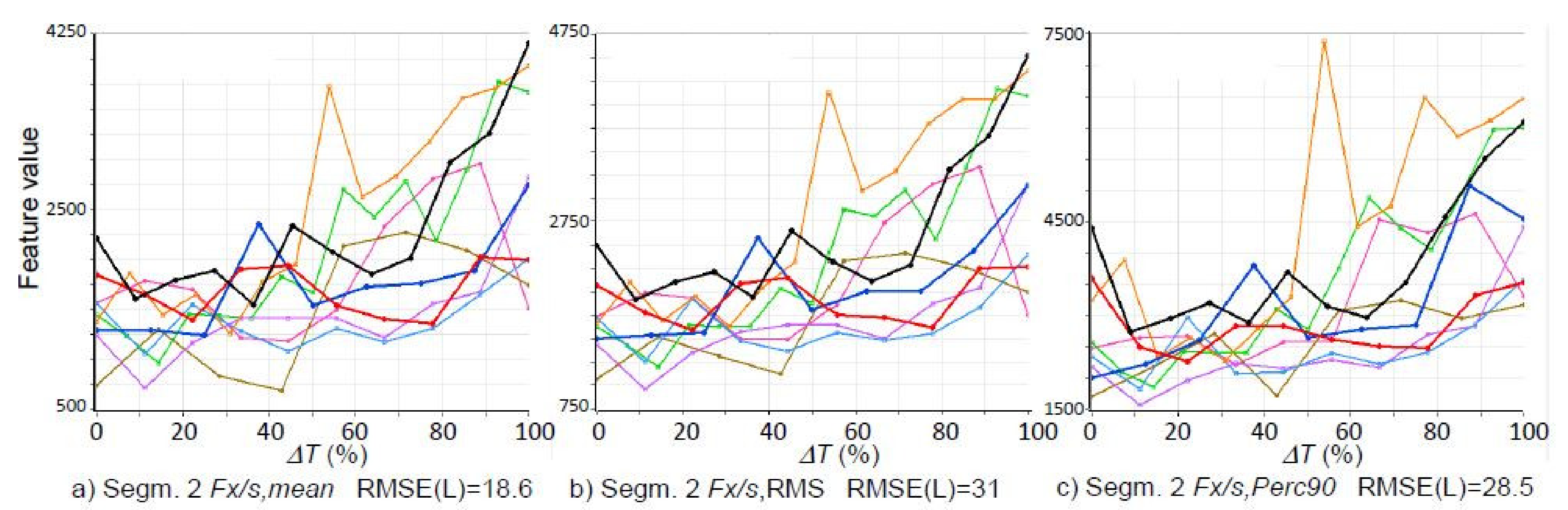
• The inter-correlation of individual SFs with each other does not necessarily occur equally in all experiments. For example, in Experiment 6, a strong correlation was found between the RMS and Perc90 values for the F_x (see Figure 7k,l) while for Experiment 1 this correlation is not so high (see Figure 7b,c).
• As shown in Figure 7j, the dependence of cutting forces on tool wear is not necessarily linear. In the case of the force signal Fx shown, its average value is negative and decreases as the tool wear increases (this is just an interpretation of the forced return by the sensor, the force is actually positive and increasing). The decrease is not linear but exponential. Cutting force proportionally translates into energy consumed in machining. It should therefore be determined experimentally for each new machining case. Determining how an increase in tool wear translates into an increase in the electricity consumed by machines will allow improvements to existing algorithms that predict machine energy consumption.

Looking at the waveforms of the SFs, it was noted that the best SFs have an RMSE(L) of less than 10. On the other hand, SFs with an RMSE(L) of more than 20 have such a high uniqueness and scatter that they can be considered unsuitable for tool condition diagnostics. In

Table 4. Number of SFs that meet criterion RMSE (L) for individual experiment.

Experiment No.	RMSE(L) <= 10		RMSE(L) <= 15		RMSE(L) <= 20
	No. of SFs	[%]	No. of SFs	[%]	No. of SFs	[%]
1	0	0.0	5	0.1	276	4.8
3	0	0.0	305	3.0	2129	20.6
5	4	0.1	182	3.2	2164	37.5
6	129	3.8	411	12.0	679	19.7

, the number of SFs below the three threshold values of RMSE(L): 10, 15 and 20 are presented. However, as the number of SFs for each experiment was different (due to a different number of sensors and segments), the percentage of SFs meeting the criterion in relation to the number of all SFs in a given experiment is also presented. For two experiments, not a single feature meeting the criterion RMSE(L) <= 10 was achieved. For experiment no. 5, four such SFs were achieved, while for experiment 6, 129 SFs were achieved, which accounted for less than 4% of all SFs. For the criterion RMSE(L) <= 15, the highest number of favorable SFs was achieved for experiment no. 6. However, for experiment no. 1, the number of SFs was only 5. After raising the criterion to 20, the number of favorable SFs for all experiments ranged from several hundred to almost 2200, which in turn may significantly increase the computation time. However, it should be considered that among the beneficial SFs there are also many SFs that are correlated with each other and this number will be significantly reduced after discarding similar SFs.

In

Table 5. The minimum value of RMSE (L) for individual SFs.

SFs/Statistical features	$\overline{\mathit{x}}$	RMS	Incr	PP	$\mathit{\sigma }$	var	${\mathit{\mu }}^3$	${\mathit{\mu }}^4$	Sk	K	Perc 90	Perc 50	CF	P
F	8	8	8	12	11	12	12	13	12	11	9	9	12	9
AErms	8	9	9	12	9	11	14	12	14	11	9	8	11	9
V	-	12	12	13	-	12	12	16	12	13	13	-	12	12
C1	-	15	15	14	-	15	15	15	14	19	13	-	17	15
C2	-	16	22	21	-	16	14	16	20	17	19	-	16	21
SFs/Statistical features	E	Shan	Count1	Count2	Count3		Pulse1	Pulse2	Pulse3	PSD, E	FFT, E	F1	F2	F3
F	8	9	12	12	11		13	11	12	13	13	16	8	23
AErms	8	10	11	12	13		10	10	13	15	15	-	-	-
V	13	12	11	13	12		12	13	11	15	15	-	-	-
C1	18	15	14	16	16		17	14	13	22	22	-	-	-
C2	18	22	14	17	13		14	18	13	26	26	-	-	-

, the minimum RMSE(L) values obtained for each feature by different sensors are presented. Looking at the results it can be seen that:

• When comparing the RMSE(L) values for the different sensors, the lowest minimum values were obtained for the force and acoustic emission sensors, while the highest values were obtained for the acoustic pressure sensor, with the dynamic sensor proving to be the most;
• Energy entropy, increment, mean value, 50th and 90th order percentile, power, RMS, Shannon entropy and F_p/F_c force ratio appeared to be the best SFs for force sensors (RMSE(L) < 10);
• The best feature for the acoustic emission sensor turned out to be (RMSE(L) < 10) Energy entropy, increment, mean value, 50th and 90th order percentile, power, RMS, Shannon entropy and standard deviation;
• For the vibration and sound pressure sensors, not a single feature was obtained for which RMSE(L) is below 10;
• Among the different SFs, the statistically largest minimum RMSE(L) values were found for: peak factor, a number of threshold crossings 2, kurtosis, fourth-order moment, Energy entropy PSD and FFT.

Of all the SFs determined for each segment of each sensor, SFs that may be correlated with each other are to be expected. Although each feature used is described by a different relationship, under certain conditions certain SFs may depend on the same physical factors and may take on similar values. The use of redundant, redundant feature values is pointless and may misrepresent the diagnostic system. It was decided to use the Pearson correlation coefficient to test for cross-correlation. After initial recognition, a value of 0.99 was taken as the threshold value. The correlation was determined for each sensor separately, for the raw signal and for the signals in the frequency domain.

The results of the cross-correlation analysis of the diagnostic signal features for the cutting force sensors are presented in

Table 6. Cross correlated SFs for machining force sensors.

Fx	Shan	RMS	mean	Pow	mom4	Perc90	Perc50	PSD.E	FFT.E
Exp 1	Pow			Shan				FFT.E	PSD.E
Exp 2	Pow	Perc50		Shan			RMS	FFT.E	PSD.E
Exp 3	Pow	mean	RMS	Shan		RMS	RMS
		Perc90	Perc90			mean	mean
		Perc50	Perc50			Perc50	Perc90
Exp 4	Pow	mean	RMS	Shan		RMS	RMS
		Perc90	Perc50				mean
		Perc50
Fy	Shan	RMS	mean	Pow	mom4	Perc90	Perc50	PSD.E	FFT.E
Exp 1	Pow	Perc90		Shan		RMS	RMS	FFT.E	PSD.E
		Perc50
Exp 2	Pow	Perc90		Shan		RMS	RMS	FFT.E	PSD.E
		Perc50				Perc50	Perc90
Exp 4	Pow	Perc90		Shan		RMS	RMS
		Perc50				Perc50	Perc90
Fz	Shan	RMS	mean	Pow	mom4	Perc90	Perc50	PSD.E	FFT.E
Exp 1	Pow	Perc90		Shan		RMS	RMS	FFT.E	PSD.E
		Perc50				Perc50	Perc90
Exp 2	Pow	Perc90		Shan		RMS	RMS	FFT.E	PSD.E
		Perc50				Perc50	Perc90
Exp 3		Perc50	Perc50	Perc50	Pulse2	Pow	mean
						Perc50	Pow
							Perc90
Exp 4	Pow	Perc90		Shan		RMS	RMS
		Perc50

. The individual cells in the table list SFs that correlate with a given feature for each experiment. SFs that do not correlate with any other feature are not listed in the tables.

The cross-correlation study of the signal features found that the features that did not correlate with other SFs, in any case, were: Energy entropy, skewness, kurtosis, interpeak value and peak factor. In contrast, regardless of sensor type, a very strong correlation was obtained between power and Shannon entropy in every experiment. Signal features that rarely correlated with other SFs were third-order moment, fourth-order moment, and threshold exceedance SFs. For cutting force sensors, the feature that did not correlate with any other feature was standard deviation.

In most cases there was also a correlation between the SFs:

• RMS, 50th percentile, 90th percentile;
• arithmetic mean and modal value;
• Energy entropy of FFT and PSD.

For the acoustic emission sensor, in most cases there was a correlation between the SFs:

• RMS, 50th order percentile, arithmetic mean value;
• Energy entropy of FFT and PSD.

For vibration and sound pressure sensors [68], in most cases there was a correlation between the SFs:

• RMS, 90th order percentile;
• Energy entropy of FFT and PSD.

3.2. Verification of Test Results

Based on the analyses presented in Section 3.1, SFs that are statistically of little use for applied tool condition diagnostics or correlated with other, better SFs were eliminated. These SFs are the Energy entropy of FFT and 10 signal SFs in the time domain and bandpass signals obtained from the WPT: peak factor, a number of crossings of thresholds 2 and 3, signal time over threshold 2 and 3, kurtosis, fourth-order moment, percentiles of 50 and 90 order, Shannon entropy. The total number of these SFs is 151, or about 46% of all SFs.

To verify the correctness of the selection and evaluation of the SFs, the results of the tool wear diagnostics for all experimental tests are presented. The learning was carried out on the first period of tool life and the rest was used for testing. The RMSE (L) <= 20 was used as the criterion for accepting the feature to estimate the tool wear. Figure 8 shows the curves of the estimated used part of the tool life ΔT_calc as a function of the actual part of the tool life ΔT_real for successive periods of tool life. Despite the limited number of SFs, very good estimation results were obtained ΔT while reducing the number of calculations.

4. Conclusions

This paper presents a universal methodology for testing the suitability of signal feature SFs for tool wear diagnostics, which can be applied to various machining operations [69]. However, the results presented for the evaluation of various SFs only apply to turning. The present study analyses the usefulness of various SFs and sensors for tool condition diagnostics for the applied method of tool wear estimation during toothing. In contrast to the studies presented so far in various publications [70,71], the present analysis of the usefulness of individual SF is comprehensive, obtained using a single methodology for determining and evaluating the SFs for many different experiments, which allows us to conclude on the universality of the obtained research results.

As a result of the research, it was noted that:

• No SF of the signal is always and under all circumstances associated with the wear of the tool. For each new machining case, many different SFs should be determined and those related to the tool state should be automatically selected from them;
• For the applied method of estimating the used part of the lifetime of the tool wear, the best SFs are irrespective of the sensor type energy entropy, increment, mean value, power and RMS as well as the standard deviation or Energy entropy of PSD. These values have both a strong correlation with the state of the tool and a low correlation with other SFs; for signals oscillating around zero or of an impulsive nature, SFs characterizing the number of times the threshold was exceeded work well and may be unrelated to those listed above.

The obtained results can be used to build a new generation of more effective tool wear diagnostics systems [72]. Such systems allow direct and indirect energy savings [73]. Indirectly by reducing the number of consumed cutting inserts and by reducing the number of defects (workpieces that are destroyed due to insert damage during machining). The latter is all the more important as machining is usually the last manufacturing technique in a production cycle. When a defect is produced, not only is the energy used in machining wasted, but also the energy used in previous production stages (casting, forging, heat treatment). Direct energy savings are achieved by avoiding cutting with a used tool, which is more energy-intensive [74]. The results obtained during experiments may also be useful for creating algorithms aimed at forecasting electricity consumption during the machining operations of specific items. At the moment, most algorithms do not consider tool wear, and those that take them into account are only determined by increasing energy consumption with total tool wear. As shown in the paper, the dependence of cutting forces (cutting force proportionally translates into energy consumed in machining) on blade wear is not necessarily linear. It should therefore be determined experimentally for each new machining case. Determining how an increase in tool wear translates into an increase in the electricity consumed by machines will allow improvements to existing algorithms that predict machine energy consumption.

References

1. Zhao, G.Y.; Liu, Z.Y.; He, Y.; Cao, H.J.; Guo, Y.B. Energy consumption in machining: Classification, prediction, and reduction strategy. Energy 2017, 133, 142–157. [Google Scholar] [CrossRef]
2. Mourtzis, D.; Vlachou, E.; Milas, N.; Dimitrakopoulos, G. Energy consumption estimation for machining processes based on real-time shop floor monitoring via wireless sensor networks. Procedia CIRP 2016, 57, 637–642. [Google Scholar] [CrossRef]
3. Mamun, A.A. Machining Strategies Exploring Reduction in Energy Consumption. Master’s Thesis, Minnesota State University, Mankato, MN, USA, 2015. [Google Scholar] [CrossRef]
4. Borgia, S.; Leonesio, M.; Pellegrinelli, S.; Valente, A. Energy driven process planning and machine tool dynamic behavior assessment. Procedia CIRP 2013, 9, 91–96. [Google Scholar] [CrossRef] [Green Version]
5. Chudy, R.; Grzesik, W. Comparison of power and energy consumption for hard turning and burnishing operations of 41Cr4 steel. J. Mach. Eng. 2015, 4, 113–120. [Google Scholar]
6. Roszkowski, A.; Piórkowski, P.; Skoczyński, W.; Borkowski, W.; Jankowski, T. Study on the Impact of Cutting Tool Wear on Machine Tool Energy Consumption. Adv. Sci. Technol. Res. J. 2020, 14, 158–164. [Google Scholar] [CrossRef]
7. Vijayraghavan, A.; Dornfeld, D. Automated energy monitoring of machine tools. Cirp Ann. Manuf. Techn. 2010, 59, 21–24. [Google Scholar] [CrossRef] [Green Version]
8. Younas, M.; Jaffery, S.H.I.; Khan, M.; Ahmad, R.; Ali, L.; Khan, Z.; Khan, A. Tool Wear Progression and its Effect on Energy Consumption in Turning of Titanium Alloy (Ti-6Al-4V). Mech. Sci. 2019, 10, 373–382. [Google Scholar] [CrossRef]
9. Warsi, S.S.; Jaffery, S.H.I.; Ahmad, R.; Khan, M.; Ali, L.; Agha, M.H.; Akram, S. Development of energy consumption map for orthogonal machining of Al 6061-T6 alloy. P. I. Mech. Eng. B J. Eng. 2018, 232, 2510–2522. [Google Scholar] [CrossRef]
10. Mativenga, P.T.; Rajemi, M.F.; Hinduja, S. Calculation of optimum cutting parameters based on minimum energy footprint. CIRP Ann.-Manuf. Techn. 2011, 60, 149–152. [Google Scholar] [CrossRef]
11. Behrendt, T.; Zein, A.; Min, S. Development of an energy consumption monitoring procedure for machine tools. CIRP Ann. Manuf. Techn. 2012, 61, 43–46. [Google Scholar] [CrossRef]
12. Kara, S.; Li, W. Unit process energy consumption models for material removal processes. CIRP Ann. Manuf. Techn. 2011, 60, 37–40. [Google Scholar] [CrossRef]
13. Kuntoglu, M.; Aslan, A.; Pimenov, D.Y.; Usca, Ü.A.; Salur, E.; Gupta, M.K.; Mikolajczyk, T.; Giasin, K.; Kapłonek, W.; Sharma, S. A Review of Indirect Tool Condition Monitoring Systems and Decision-Making Methods in Turning: Critical Analysis and Trends. Sensors 2021, 21, 108. [Google Scholar] [CrossRef]
14. Yuan, J.; Liu, L.; Yang, Z.; Zhang, Y. Tool Wear Condition Monitoring by Combining Variational Mode Decomposition and Ensemble Learning. Sensors 2020, 20, 6113. [Google Scholar] [CrossRef] [PubMed]
15. Bombiński, S.; Kossakowska, J.; Nejman, M.; Haber, R.E.; Castaño, F.; Fularski, R. Needs, Requirements and a Concept of a Tool Condition Monitoring System for the Aerospace Industry. Sensors 2021, 21, 5086. [Google Scholar] [CrossRef] [PubMed]
16. Balsamo, V.; Caggiano, A.; Jemielniak, K.; Kossakowska, J.; Nejman, M.; Teti, R. Multi Sensor Signal Processing for Catastrophic Tool Failure Detection in Turning. Procedia CIRP 2016, 41, 939–944. [Google Scholar] [CrossRef]
17. Digital Way Group, Tool Wear & Breakage Monitoring System. Available online: https://www.digitalway.fr/cutting-tool-monitoring/why-buy-wattpilote/ (accessed on 23 July 2021).
18. DMG MORI, Easy Tool Monitoring 2.0. Available online: https://pl.dmgmori.com/produkty/digitization/integrated-digitization/production/cykle-technologiczne/easy-tool-monitoring-2-0 (accessed on 23 July 2021).
19. Bombiński, S.; Kossakowska, J.; Jemielniak, K. Detection of accelerated tool wear in turning. Mech. Syst. Signal. Process. 2022, 162, 108021. [Google Scholar] [CrossRef]
20. Jemielniak, K. Contemporary challenges in tool condition monitoring. J. Mach. Eng. 2019, 19, 48–61. [Google Scholar] [CrossRef]
21. Heinemann, R.; Hinduja, S. A new strategy for tool condition monitoring of small diameter twist drills in deep-hole drilling. Int. J. Mach. Tools Manuf. 2012, 52, 69–76. [Google Scholar] [CrossRef]
22. Beruvides, G.; Quiza, R.; del Toro, R.; Haber, R.E. Sensoring systems and signal analysis to monitor tool wear in microdrilling operations on a sintered tungsten–copper composite material. Sens. Actuators A Phys. 2013, 199, 165–175. [Google Scholar] [CrossRef]
23. Ai, C.S.; Sun, Y.J.; He, G.W.; Ze, X.B.; Li, W.; Mao, K. The milling tool wear monitoring using the acoustic spectrum. Int. J. Adv. Manuf. Technol. 2012, 61, 457–463. [Google Scholar] [CrossRef]
24. Elangovan, M.; Devasenapati, S.B.; Sakthivel, N.R.; Ramachandran, K.I. Evaluation of expert system for condition monitoring of a single point cutting tool using principle component analysis and decision tree algorithm. Expert Syst. Appl. 2011, 38, 4450–4459. [Google Scholar] [CrossRef]
25. Ding, F.; He, Z. Cutting tool wear monitoring for reliability analysis using proportional hazards model. Int. J. Adv. Manuf. Technol. 2011, 57, 565–574. [Google Scholar] [CrossRef]
26. Wang, J.; Wang, P.; Gao, R.X. Tool life prediction for sustainable manufacturing. In Proceedings of Innovative Solutions, Proceedings of the 11th Global Conference on Sustainable Manufacturing, Berlin, Germany, 23–25 September 2013; Universitätsverlag der TU Berlin: Berlin, Germany, 2013. Available online: https://depositonce.tu-berlin.de/bitstream/11303/5023/1/wang_wang_gao.pdf (accessed on 27 September 2021).
27. Jemielniak, K.; Urbański, T.; Kossakowska, J.; Bombiński, S. Tool condition monitoring based on numerous signal features. Int. J. Adv. Manuf. Technol. 2012, 59, 73–81. [Google Scholar] [CrossRef] [Green Version]
28. Cho, S.; Binsaeid, S.; Asfour, S. Design of multisensor fusion-based tool condition monitoring system in end milling. Int. J. Adv. Manuf. Technol. 2010, 46, 681–694. [Google Scholar] [CrossRef]
29. Patra, K.; Pal, S.K.; Bhattacharyya, K. Fuzzy radial basis function (FRBF) network based tool condition monitoring system using vibration signals. Mach. Sci. Technol. 2010, 14, 280–300. [Google Scholar] [CrossRef]
30. Painuli, S.; Elangovan, M.; Sugumaran, V. Tool condition monitoring using K-star algorithm. Expert Syst. Appl. 2014, 41, 2638–2643. [Google Scholar] [CrossRef]
31. Silva, R.G. Condition monitoring of the cutting process using a self-organizing spiking neural network map. J. Intell. Manuf. 2010, 21, 823–829. [Google Scholar] [CrossRef]
32. Wang, G.; Cui, Y. On line tool wear monitoring based on auto associative neural network. J. Intell. Manuf. 2013, 24, 1085–1094. [Google Scholar] [CrossRef]
33. Dong, J.; Hong, G.S.; Wong, Y.S. Bayesian support vector regression for tool condition monitoring and feature selection. 2004. Available online: http://www.icsc.ab.ca/conferences/eis2004/Conf/41.pdf (accessed on 27 September 2021).
34. Wang, G.; Yang, Y.; Xie, Q.; Zhang, Y. Force based tool wear monitoring system for milling process based on relevance vector machine. Adv. Eng. Softw. 2014, 71, 46–51. [Google Scholar] [CrossRef]
35. Jemielniak, K.; Kossakowska, J.; Urbański, T. Application of wavelet transform of acoustic emission and cutting force signals for tool condition monitoring in rough turning of Inconel 625. Proc. Inst. Mech. Eng. Part. B J. Eng. Manuf. 2011, 225, 123–129. [Google Scholar] [CrossRef]
36. Jemielniak, K.; Kossakowska, J. Tool wear monitoring based on wavelet transform of raw acoustic emission signal. Adv. Manuf. Sci. Technol. 2010, 34, 5–16. Available online: http://yadda.icm.edu.pl/yadda/element/bwmeta1.element.baztech-article-BOS5-0025-0001 (accessed on 27 September 2021).
37. Liu, T.I.; Kumagai, A.; Wang, Y.C.; Song, S.D.; Fu, Z.; Lee, J. On-line monitoring of boring tools for control of boring operations. Robot. Comput. Integr. Manuf. 2010, 26, 230–239. [Google Scholar] [CrossRef]
38. Ren, Q.; Balazinski, M.; Jemielniak, K.; Baron, L.; Achiche, S. Experimental and fuzzy modelling analysis on dynamic cutting force in micro milling. Soft Comput. 2013, 17, 1687–1697. [Google Scholar] [CrossRef]
39. Zhou, J.H.; Pang, C.K.; Zhong, Z.W.; Lewis, F.L. Tool wear monitoring using acoustic emissions by dominant-feature identification. IEEE Trans. Instrum. Meas. 2011, 60, 547–559. [Google Scholar] [CrossRef]
40. Ali, Y.H.; Rahman, R.A.; Hamzah, R.I.R. Acoustic emission signal analysis and artificial intelligence techniques in machine condition monitoring and fault diagnosis: A review. J. Teknol. 2014, 69, 121–126. [Google Scholar] [CrossRef] [Green Version]
41. Wang, G.; Yang, Y.; Guo, Z. Hybrid learning based Gaussian ARTMAP network for tool condition monitoring using selected force harmonic features. Sens. Actuators A Phys. 2013, 203, 394–404. [Google Scholar] [CrossRef]
42. Wilkowski, J.; Górski, J. Vibro-acoustic signals as a source of information about tool wear during laminated chipboard milling. Wood Res. 2011, 56, 57–66. Available online: http://www.woodresearch.sk/wr/201101/06.pdf (accessed on 27 September 2021).
43. Wang, G.; Guo, Z.; Yang, Y. Force sensor based online tool wear monitoring using distributed Gaussian ARTMAP network. Sens. Actuators A Phys. 2013, 192, 111–118. [Google Scholar] [CrossRef]
44. Lu, P.; Chou, Y.K.; Thompson, R.G. Short-Time Fourier Transform method in AE signal analysis for diamond coating failure monitoring in machining applications. In Proceedings of the ASME 2010 International Manufacturing Science and Engineering Conference, Erie, PA, USA, 12–15 October 2010. [Google Scholar] [CrossRef]
45. Raja, J.E.; Kiong, L.C.; Soong, L.W. Hilbert–Huang transform-based emitted sound signal analysis for tool flank wear monitoring. Arab. J. Sci. Eng. 2013, 38, 2219–2226. [Google Scholar] [CrossRef]
46. Raja, J.E.; Lim, W.S.; Venkataseshaiah, C. Emitted sound analysis for tool flank wear monitoring using Hilbert Huang Transform. Int. J. Comput. Electr. Eng. 2012, 4, 110–114. Available online: http://www.ijcee.org/papers/460-E1224.pdf (accessed on 27 September 2021). [CrossRef] [Green Version]
47. Pal, S.; Heyns, P.S.; Freyer, B.H.; Theron, N.J.; Pal, S.K. Tool wear monitoring and selection of optimum cutting conditions with progressive tool wear effect and input uncertainties. J. Intell. Manuf. 2011, 22, 491–504. [Google Scholar] [CrossRef] [Green Version]
48. Freyer, B.H.; Heyns, P.S.; Theron, N.J. Comparing orthogonal force and unidirectional strain component processing for tool condition monitoring. J. Intell. Manuf. 2014, 25, 473–487. [Google Scholar] [CrossRef] [Green Version]
49. Wang, G.F.; Yang, Y.W.; Zhang, Y.C.; Xie, Q.L. Vibration sensor based tool condition monitoring using ν support vector machine and locality preserving projection. Sens. Actuators A Phys. 2014, 209, 24–32. [Google Scholar] [CrossRef]
50. Cai, G.; Chen, X.; Li, B.; Chen, B.; He, Z. Operation reliability assessment for cutting tools by applying a proportional covariate model to condition monitoring information. Sensors 2012, 12, 12964–12987. [Google Scholar] [CrossRef] [PubMed] [Green Version]
51. Gómez, M.P.; Hey, A.M.; D’Attelis, C.E.; Ruzzante, J.E. Assessment of cutting tool condition by acoustic emission. Procedia Mater. Sci. 2012, 1, 321–328. [Google Scholar] [CrossRef] [Green Version]
52. Rangwala, S.; Dornfeld, D.A. Sensor Integration Using Neural networks for intelligent tool conditioning monitoring. J. Eng. Ind. 1990, 112, 219–228. [Google Scholar] [CrossRef]
53. Silva, R.; Araújo, A. A novel approach to condition monitoring of the cutting process using recurrent neural networks. Sensors 2020, 20, 4493. [Google Scholar] [CrossRef] [PubMed]
54. Ou, J.; Li, H.; Huang, G.; Zhou, Q. A novel order analysis and stacked sparse auto-encoder feature learning method for milling tool wear condition monitoring. Sensors 2020, 20, 2878. [Google Scholar] [CrossRef]
55. Zhou, J.M.; Andersson, M.; Stahl, J.E. The monitoring of flank wear on the CBN tool in the hard turning process. Int. J. Adv. Manuf. Technol. 2003, 22, 697–702. [Google Scholar] [CrossRef]
56. Jemielniak, K.; Kwiatkowski, L.; Wrzosek, P. Ocena przydatności miar emisji akustycznej i sił skrawania do diagnostyki stanu narzędzia przy toczeniu. Postępy Technol. Masz. I Urządzeń 1997, 212, 25–36. Available online: http://www.zaoios.pw.edu.pl/kjemiel/docs/OcenaMiarFiAE.pdf (accessed on 27 September 2021).
57. Zhu, K.; Wong, Y.; Hong, G. Multi-category micro-milling tool wear monitoring with continuous hidden markov models. Mech. Syst. Signal. Process. 2009, 23, 547–560. [Google Scholar] [CrossRef]
58. Sokołowski, A.; Kosmol, J. Designing intelligent diagnostic systems. In Proceedings of the International Conference on Computer Integrated Manufacturing—CIM 96, Zakopane, Poland, 14–17 May 1996; Volume I. [Google Scholar]
59. Zhang, C.; Yao, .; Zhang, J.; Jin, H. Tool condition monitoring and remaining useful life prognostic based on a wireless sensor in dry milling operations. Sensors 2016, 16, 795. [Google Scholar] [CrossRef] [PubMed] [Green Version]
60. Caggiano, A.; Rimpault, X.; Teti, R.; Balazinski, M.; Chatelain, J.F.; Nele, L. Machine learning approach based on fractal analysis for optimal tool life exploitation in CFRP composite drilling for aeronautical assembly. CIRP Ann. Manuf. Technol. 2018, 67, 483–486. [Google Scholar] [CrossRef]
61. Jemielniak, K.; Kwiatkowski, L.; Wrzosek, P. Diagnosis of tool wear based on cutting forces and AE features as inputs to Neural Network. J. Intell. Manuf. 1998, 9, 447–455. [Google Scholar] [CrossRef]
62. Xie, Z.; Li, J.; Lu, Y. Feature selection and a method to improve the performance of tool condition monitoring. Int. J. Adv. Manuf. Technol. 2019, 100, 3197–3206. [Google Scholar] [CrossRef]
63. Al-Habaibeh, A.; Gindy, N. Self-learning algorithm for automated design of condition monitoring systems for milling operations. Int. J. Adv. Manuf. Technol. 2001, 18, 448–459. [Google Scholar] [CrossRef]
64. Al-Habaibeh, A.; Zorriassatine, F.; Gindy, N. Comprehensive experimental evaluation of a systematic approach for cost effective and rapid design of condition monitoring systems using Taguchi’s method. J. Mater. Process. Technol. 2002, 124, 372–383. [Google Scholar] [CrossRef]
65. Zązel, Z.; Sokołowski, A. Próba Zastosowania Inteligentnego Narzędzia do Procesu Wiercenia. Prace Naukowe Katedry Budowy Maszyn nr 4, Gliwice. 2002. Available online: http://yadda.icm.edu.pl/baztech/element/bwmeta1.element.baztech-article-BSL7-0010-0003 (accessed on 27 September 2021).
66. Bombiński, S.; Błażejak, K.; Nejman, M.; Jemielniak, K. Sensor signal segmentation for tool condition monitoring. Procedia CIRP 2016, 46, 155–160. [Google Scholar] [CrossRef] [Green Version]
67. Jemielniak, K. Tool wear monitoring based on a non-monotonic signal feature. J. Eng. Manufacture. Part. B 2006, 220, 163–170. [Google Scholar] [CrossRef]
68. Liu, M.-K.; Tseng, Y.-H.; Tran, M.-Q. Tool wear monitoring and prediction based on sound signal. Int. J. Adv. Manuf. Technol 2019, 103, 3361–3373. [Google Scholar] [CrossRef]
69. Waydande, P.; Ambhore, N.; Chinchanikar, S. A Review on Tool Wear Monitoring System. J. Mech. Eng. Autom. 2016, 6, 49–53. [Google Scholar] [CrossRef]
70. Antsev, A.V.; Zhmurin, V.V.; Yanov, E.S.; Dang, T.H. Cutting tool wear monitoring using the diagnostic capabilities of modern CNC machines. J. Phys. Conf. Ser. 2019, 1260, 032003. [Google Scholar] [CrossRef]
71. Benkedjouh, T.; Zerhouni, N.; Rechak, S. Tool wear condition monitoring based on continuous wavelet transform and blind source sep. Int. J. Adv. Manuf. Technol. 2018, 97, 3311–3323. [Google Scholar] [CrossRef]
72. Cao, X.; Chen, B.; Yao, B.; Zhuang, S. An Intelligent Milling Tool Wear Monitoring Methodology Based on Convolutional Neural Network with Derived Wavelet Frames Coefficient. Appl. Sci. 2019, 9, 3912. [Google Scholar] [CrossRef] [Green Version]
73. Luan, X.; Zhang, S.; Li, J.; Mendis, G.; Zhao, F.; Sutherland, J.W. Trade-off analysis of tool wear, machining quality and energy efficiency of alloy cast iron milling process. Procedia Manuf. 2018, 26, 383–393. [Google Scholar] [CrossRef]
74. Liu, Z.Y.; Guo, Y.B.; Sealy, M.P.; Liu, Z.Q. Energy consumption and process sustainability of hard milling with tool wear progression. J. Mater. Process. Technol. 2016, 229, 305–312. [Google Scholar] [CrossRef]
Figure 1. The general structure of a tool and cutting process diagnostic system.
Energies 14 06489 g001
Figure 2. Signal processing logical scheme.
Energies 14 06489 g002
Figure 3. Three-level WPT decomposition; blackened fields indicate the frequency band of the original signal.
Energies 14 06489 g003
Figure 4. Machining patterns in Experiments 1–4.
Energies 14 06489 g004
Figure 5. Variance vs. energy entropy values for exemplary signals.
Energies 14 06489 g005
Figure 6. The waveforms of the force signal Fz (Experiment 3). (a) original signal (b), the band signals obtained from the WPT—package AAA (c) the band signals obtained from the WPT—package DDD.
Energies 14 06489 g006
Figure 7. Exemplary courses of SFs obtained for experiment 1 (ac), experiment 2 (df), experiment 3 (gi) and experiment 4 (jl).
Energies 14 06489 g007aEnergies 14 06489 g007b
Figure 8. Estimated toollife from learning on selected signal features.
Energies 14 06489 g008