Design and Implementation of Frequency Controller for Wind Energy-Based Hybrid Power System Using Quasi-Oppositional Harmonic Search Algorithm

Abstract

An innovative union of fuzzy controller and proportional-integral-derivative (PID) controller under the environment of fractional order (FO) calculus is described in the present study for an isolated hybrid power system (IHPS) in the context of load frequency control. The proposed controller is designated as FO-fuzzy PID (FO-F-PID) controller. The undertaken model of IHPS presented here involves different independent power-producing units, a wind energy-based generator, a diesel engine-based generator and a device for energy storage (such as a superconducting magnetic energy storage system). The selection of the system and controller gains was achieved through a unique quasi-oppositional harmony search (QOHS) algorithm. The QOHS algorithm is based on the basic harmony search (HS) algorithm, in which the combined concept of quasi-opposition initialization and HS algorithm fastens the profile of convergence for the algorithm. The competency and potency of the intended FO-F-PID controller were verified by comparing its performance with three different controllers (integer-order (IO)-fuzzy-PID (IO-F-PID) controller, FO-PID and IO-PID controller) in terms of deviation in frequency and power under distinct perturbations in load demand conditions. The obtained simulation results validate the cutting-edge functioning of the projected FO-F-PID controller over the IO-F-PID, FO-PID and IO-PID controllers under non-linear and linear functioning conditions. In addition, the intended FO-F-PID controller, considered a hybrid model, proved to be more robust against the mismatches in loading and the non-linearity in the form of rate constraint under the deviation in frequency and power front.

1. Introduction

A number of studies have confirmed that the availability of electricity to communities can deliver several socio-economic gains such as a superior education system, effective business models and better healthcare opportunities [1,2]. The energy crisis in developing countries affects nearly 2 billion people who have no access to electric energy due to the absence of an electric grid in their regions. Moreover, electricity in underdeveloped regions lacks reliability—this not only means that the lights sometimes flicker, but also that the complete region can be left in darkness for hours and even days on end. The solution lies in the existence of the grid; however, the establishment of grids for many of these locations is impractical as most of the population is scattered, living in a harsh landscape or both. Hence, the population in these regions generally have to depend on diesel engine generators (DEGs) for electricity [3]. However, this is a very costly and complex affair as it involves huge costs such as transportation costs for the fuel and other associated complications related to energy such as oil price escalation, global warming, global environmental challenges, etc. These challenges along with the energy requirement demand make small stand-alone renewable energy systems (RESs) essential [4].

RESs (such as wind and solar) are the only substitute for fossil fuels. At present, solar photovoltaic and wind energy systems can provide electricity to a majority of individual systems. However, when compared, the energy conversion proficiency of wind energy systems is higher than that of solar photovoltaic systems. Consequently, wind energy systems have an advantage over solar photovoltaic systems [5].

Wind energy-based generators (WTGs) produce power with shifting frequencies and magnitudes due to irregular attributes from wind energy [4] that interrupt the reliability and stability of the local network [6]. However, these problems related to WTGs may be prevented by hybridizing WTGs with DEGs. The local network undertaken in the current study is categorized as an isolated hybrid power system (IHPS) [7] since it is not connected to the grid.

In the case of WTG failure, the DEG takes control whenever there is a mismatch in the power generation and load demand for IHPS. In a DEG, the fuel ejection system may be fueled by the operational load and the switching frequency. The operation of DEG is not satisfactory when there is frequent switching action and lower load demand. The solution lies in the utilization of energy storage devices (ESDs) along with WTGs and DEGs in IHPS [6]. In conditions with a lower speed of wind or load peak demand, the unconsumed active energy stored by the ESDs (flywheel energy storage system, battery energy storage system, compressed air energy storage, supercapacitors, superconducting magnetic energy storage (SMES), etc.) is made available [8]. However, from the available ESDs catalogue, SMES have the quickest and extremely adaptable control functioning. In [9], SMES is employed for suppressing the power and frequency due to load perturbation in IHPS. A potent design of SMES for an IHPS with a wind-diesel generation unit has been suggested with the standard lag/lead compensator of predefined configuration [10]. Several studies have been carried out that prove the potential of SMES units for IHPS application and hence, a controlling strategy that will synchronize with distinct energy sources for accurate functioning of the system is necessary.

Currently, the primary problem of the IHPS lies in the difficulty associated with the process of controlling the wind speed deviations of a wind turbine (as its power output holds the cubic relation to the wind velocity) and the demanded load. Largely, classical controller tuning is engaged for IHPS controlling, such as proportional-integral (PI) controller, proportional-derivative (PD) controller, proportional-integral-derivative (PID) controllers, etc. However, the sensitivity of the classical controllers concerning load variations, system parametric variations, etc., is high. Thus, in order to resolve this problem associated with controlling the action, wind energy conversion is generally carried out utilizing a fuzzy logic controller (FLC) [11], as proposed by Zadeh [12]. However, the FLC has design deficiencies and still the standards are not well-defined for (a) membership functions (MFs) design, (b) rule base pattern, (c) number of considered linguistic divisions, (d) defuzzification methodology, and (e) appropriate inference mechanism. Generally, in designers’ experiences, the method of hit and trial is utilized for a selection of these parameters. Therefore, new practices for resolving these complexities of FLC design are required. In [13], the PID controller is hybridized with FLC for improving its utilization capabilities and controlling the action. Carvajal et al. [14] discussed a controller structure combining the PID controller with FLC and specified its capability of handling systems with non-linear, higher-order uncertainty, as well as complex systems. Furthermore, the differentiation and integration (differ-integral) operators provide additional flexibility in design with the combination of fractional order (FO), proving its competency as an improved estimator for the control signals compared to the integer order (IO). The primary idea for the insertion of the input and output FO operators of the FLCs is based on the heuristic understanding of a confident rate of change in error. This degree of change in error as perceived through the operator and a comparable activity can be carried out and cannot be invariable in nature [15].

In recent years, the demand for fractional calculus-based control systems amongst researchers has increased manifold because of its added features of being flexible and high-functioning. Podlubny [16] expanded the logic of the classical PID controller by utilizing the concept of FO differ-integral to the FO-PID controller by proposing two new scales of freedom: the orders of the integrator (λ) and differentiator (µ). Owing to the features of high flexibility and greater adjustment property, the FO-PID controllers find their application within the realm of various control schemes for controlling energy in wind-driven generators [17], nuclear power plants [18] and water-driven generators [19]. Furthermore, the FO-based fuzzy-PID (F-PID) (FO-F-PID) controller is broadly applied for controlling systems with non-linear, time-varying and vague characteristics. To handle the oscillatory FO processes, the FO-F-PID control with the tuning process based on the optimal time domain is projected in [20,21].

From the literature survey, it can be stated that among all the controllers, from the perspective of superior performance and robustness, the FO-F-PID controller has an edge. An FO-based control structure for the IHPS model is explored in the present study, inspired by the diversified applications of FO control systems based on computational intelligence for various power systems with the automatic regulation of voltage [22], frequency deviation suppression on the two-area system under load perturbation [23] and control of frequency in microgrid configurations [24].

In [25], the HS algorithm’s amended version is proposed for upgrading the convergence shape by introducing a reasonable optimal global solution in real-time. The swarm intelligence perception has been exploited to realize a global best HS algorithm [26]. Mahdavi et al. proposed amending its crucial variables dynamically to achieve a better HS algorithm [27]. In [28], Banerjee et al. applied the opposition-reflected learning concept for the opposition-based HS (OHS) algorithm in the optimizing problem for the compensation of reactive power in IHPS. Similarly, by applying the concept of quasi-oppositional learning to the fundamental algorithm of HS, the developed algorithm is the quasi-oppositional harmony search (QOHS) algorithm, which is utilized in IHPS to stabilize the deviation of frequency in [29]. Therefore, in the current study, the newest and effective QOHS algorithm [29] is implemented with the view of controlling the deviation in power flow alongside the variation by optimal tunning of the vital optimizable variables of the considered IHPS on its installed controllers and ESD.

Given the aforementioned literature survey, the core motivation of the current study evolves with the subsequent considerations.

(a)

For the end-users, an alternative source of electricity may be the modelling of an IHPS.

(b)

For delivering the uninterrupted power supply for the ultimate consumer with quality, the appropriateness of SMES as an ESD may be investigated.

(c)

In designing the controller, the effectiveness of both FO calculus and IO calculus may be studied and the most suitable one may be adopted.

(d)

A new modified HS algorithm considers the concept of quasi-oppositional learning, i.e., the QOHS algorithm, recognized for efficient optimization process in regulating the deviations of frequency and power. This may be achieved by appropriately optimizing the vital optimizable variables of the IHPS system under study.

Therefore, the major contributions of the study are as follows.

The present study makes an effort to:

(a)

Improve the stability and reliability of IHPS (consists of WTG, DEG and SMES) for rural as well as urban areas with nil effects on the environment.

(b)

Enhance the quality of governor-regulated DEG supply power and the pitch-controlled WTG power output together with power obtained from SMES.

(c)

Implement the theory of fractional calculus for controller design to regulate its working principle.

(d)

Enhance the objective function-based convergence profile while employing the QOHS algorithm (a new HS algorithm variant, inspired by the concept of quasi-oppositional learning) for optimizing the tuning purpose of the optimizable variables of the controllers with additional vital variables of the system under study.

(e)

Evaluating the efficacy of the system while dealing with ambiguities, random load demand deviation and stochastic variation in step.

(f)

Analyze the QOHS algorithm and controllers’ robustness. Furthermore, the system robustness is also verified with load mismatch variation and the insertion of rate constraint-type non-linearity.

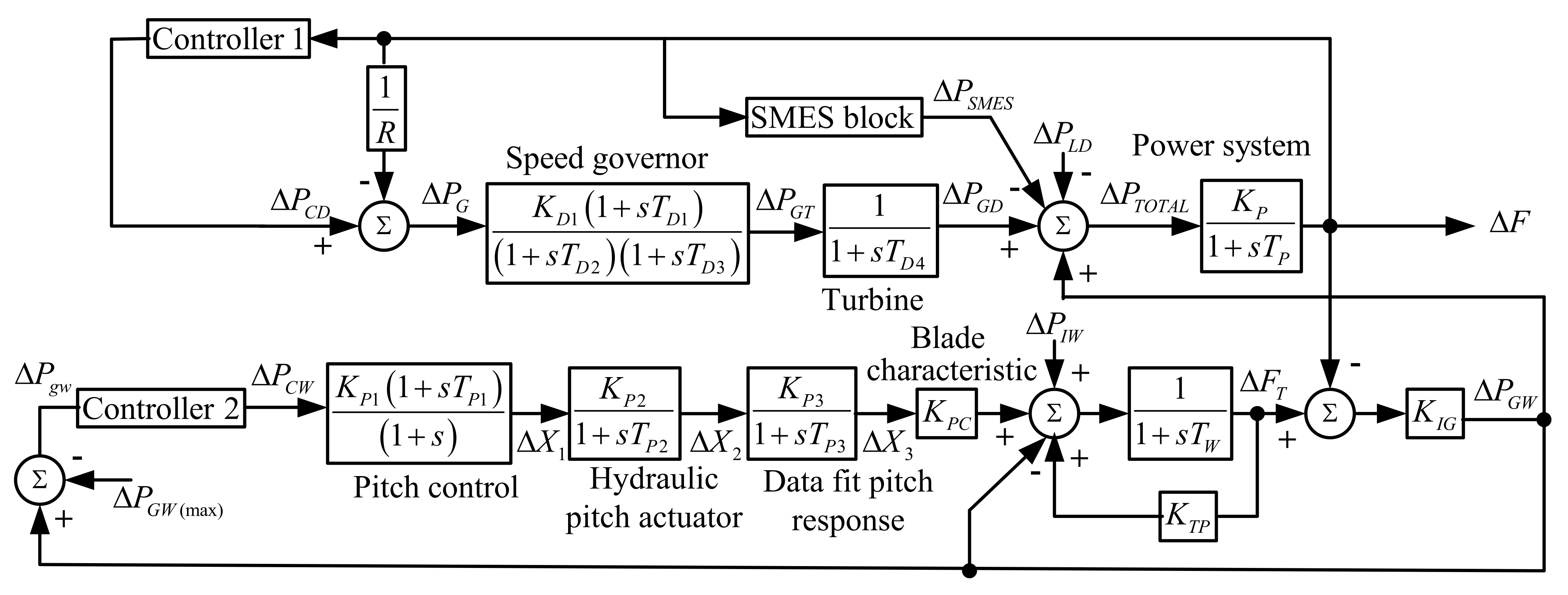
The proposed work is presented in a flow chart manner in Figure 1, representing the whole idea and work contained in the manuscript in a step-by-step manner.

The manuscript is organized as follows. Section 2 describes important elements of the IHPS. In Section 3, architecture and the concept of FO and IO controllers are explained. The details of the optimization task and objective function are illuminated in Section 4. In Section 5, the base variant and adaptation incorporated in the basic HS algorithm to form the QOHS algorithm are demonstrated. The analysis of the simulation results is presented in Section 6. Finally, in Section 7, the present work is concluded.

2. System Model

In the studied IHPS, during its regular operation, undergoes a minor deviation in the load demand. Hence for the analysis of the IHPS model linear model has been undertaken for dynamic illustration [10]. Consequently, for the studied IHPS (a wind turbine generator (WTG), a DEG and an ESD (a SMES device)), the schematic block diagram of the considered model based on transfer functions (TF/TFs) is depicted in Figure 2 with the installed controllers. The rated capacity of 150 kW is chosen for both the WTG and the DEG respectively and the nominal system parameters are furnished from [28,29,30].

The variations in frequency and power in this studied IHPS, are reduced by the collective work of the SMES, the DEG speed governor and the devoted support of the WTG pitch controller. For the considered IHPS arrangement (Figure 2), the overall variation in the entire power output $\left(\mathsf{\Delta }{P}_{TOTAL}\right)$ is evaluated using Equation (1):

$$\mathsf{\Delta }{P}_{TOTAL}=\mathsf{\Delta }{P}_{DEG}+\mathsf{\Delta }{P}_{WTG}-\mathsf{\Delta }{P}_{SMES}-\mathsf{\Delta }{P}_{LD}$$

(1)

In Equation (1), $\mathsf{\Delta }{P}_{TOTAL}$, $\mathsf{\Delta }{P}_{DEG}$, $\mathsf{\Delta }{P}_{WTG}$, $\mathsf{\Delta }{P}_{SMES}$ and $\mathsf{\Delta }{P}_{LD}$ represent the change in total power, DEG power, WTG power output, the power output of the SMES and input load demand, respectively.

2.1. Wind Turbine Generator (WTG)

The WTG-generated power is governed by the wind speed available to the wind turbine. The wind speed is subjected to variables involving maximum, rated, or zero output power [31], depicted in (2):

$$P_{WTG}=\left\{\begin{array}{l}\left(V^2-V_{c\_in}^2/V_r^2-V_{c\_in}^2\right)\left(P_{rat}\right);\hspace{1em}{V}_{c\_in}\le V\le V_{rat}\\ P_{rat};\hspace{1em}\hspace{1em}\hspace{1em}\hspace{1em}\hspace{1em}\hspace{1em}\hspace{1em}\hspace{1em}\hspace{1em}{V}_{rat}\le V\le V_{c\_out}\\ 0;\hspace{1em}\hspace{1em}\hspace{1em}\hspace{1em}\hspace{1em}\hspace{1em}\hspace{1em}\hspace{1em}\hspace{1em}V\le V_{c\_in }and\hspace{1em}V\ge V_{c\_out}\end{array}\right.$$

(2)

where $P_{rat}$ is the rated output power, $V_{c\_in}$ is the wind cut-in speed, $V_r$ is the wind-rated speed and $V_{c\_out}$ is the wind cut-off speed. When the wind speed changes, a standard WTG generates power that varies from $V_{c\_in}$ to $V_{c\_out}$ that leads to a linear increase in the generated power [31]. The pitching action creates non-linearity to support the WTG speed. The WTG is rationalized to a first-order system and denoted as the TF from (3)–(7):

$$\mathsf{\Delta }F=\left(\frac{K_P}{1+s{T}_P}\right)\left[\mathsf{\Delta }{P}_{DEG}+\mathsf{\Delta }{P}_{WTG}-\mathsf{\Delta }{P}_{SMES}-\mathsf{\Delta }{P}_{LD}\right]$$

(3)

$$\mathsf{\Delta }{P}_{DEG}=K_{FC}\left[\mathsf{\Delta }{F}_T-\mathsf{\Delta }F\right]$$

(4)

$$\mathsf{\Delta }{F}_T=\left(\frac{1}{1+s{T}_W}\right)\left[K_{TP}\mathsf{\Delta }{F}_T-\mathsf{\Delta }{P}_{GW}+K_{PC}\mathsf{\Delta }{X}_3+\mathsf{\Delta }{P}_{IW}\right]$$

(5)

$$\mathsf{\Delta }{X}_3=\mathsf{\Delta }{P}_{CW}\left[\frac{K_{PA}{K}_{PB}{K}_{PC}\left(1+s{T}_{PA}\right)}{\left(1+s\right)\left(1+s{T}_{PB}\right)\left(1+s{T}_{PC}\right)}\right]$$

(6)

$$\mathsf{\Delta }{P}_{CW}=\left[\mathrm{The}\mathrm{transfer}\mathrm{function}\mathrm{of}\mathrm{controller}2\right]=\left(\mathsf{\Delta }{P}_{DEG}-\mathsf{\Delta }{P}_{DEG(max)}\right)$$

(7)

where $K_P$, $K_{FC}$, $K_{PC}$, $K_{PA}$ and $K_{PB}$ are the gains of the data fit pitch response, the hydraulic pitch actuator, the pitch control, the blade characteristic and fluid coupling, $T_{PA}$ (pitch controller time constant), $T_{PB}$ (hydraulic pitch actuator time constant) and $T_{PC}$ (data fit pitch time constant), respectively, while the $\mathsf{\Delta }F$ represents the frequency deviation of the system. Hence, the value of $\mathsf{\Delta }{P}_{DEG}$ can be estimated as in Equation (1).

2.2. Diesel Engine Generators (DEG)

For the DEG model, the speed of the generator along with the mechanical output power from the engine are described as the function of fuel consumption rate (FCR) [32]. The FCR of the DEG can be indicated as (8):

$$Q\left(t\right)={\alpha }_{GED}P{\left(t\right)}_{GED.gen}+{\beta }_{GED}P{\left(t\right)}_{GED.rat}$$

(8)

where ${\alpha }_{GED}$ (per kWh) and ${\beta }_{GED}$ (per kWh) represent the coefficients from the fuel consumption curve and $Q\left(t\right)$ is the fuel consumption of DEG on an hourly basis, made available from the maker. Furthermore, $P{\left(t\right)}_{GED.gen}$ (kW) is the DEG-generated power and $P{\left(t\right)}_{GED.rat}$ (kW) is the DEG-rated power. Here, it should be noted that non-linearity in a DEG exists by virtue of the dead time, which is the time-varying nature between the mechanical torque production and fuel injection. The relation between engine mechanical power and fuel consumption is illustrated in [33] where a simple first-order TF model for DEG has been considered, as in Figure 2, and may be described as:

$$\mathsf{\Delta }{P}_{GED}=\left(\frac{1}{1+s{T}_{DT}}\right)\mathsf{\Delta }{P}_{GT}$$

(9)

$$\mathsf{\Delta }{P}_{GT}=\left(\frac{K_{DA}\left(1+s{T}_{DA}\right)}{\left(1+s{T}_{DB}\right)\left(1+s{T}_{DC}\right)}\right)\mathsf{\Delta }{P}_G$$

(10)

$$\mathsf{\Delta }{P}_G=\mathsf{\Delta }{P}_{CD}-\frac{1}{R}\mathsf{\Delta }F=\left[\left\{ Controller\mathrm{1}\mathrm{Transfer}\mathrm{function}\right\}-\frac{1}{R}\right]\mathsf{\Delta }F$$

(11)

where $K_{DA}$ is the gain of the speed governor, $T_{DA}$, $T_{DB}$ and $T_{DC}$ are the speed governor time constants and $T_{DT}$ is the turbine time constant. Hence, the calculation of $\mathsf{\Delta }{T}_{GD}$ in Equation (1) can be carried out.

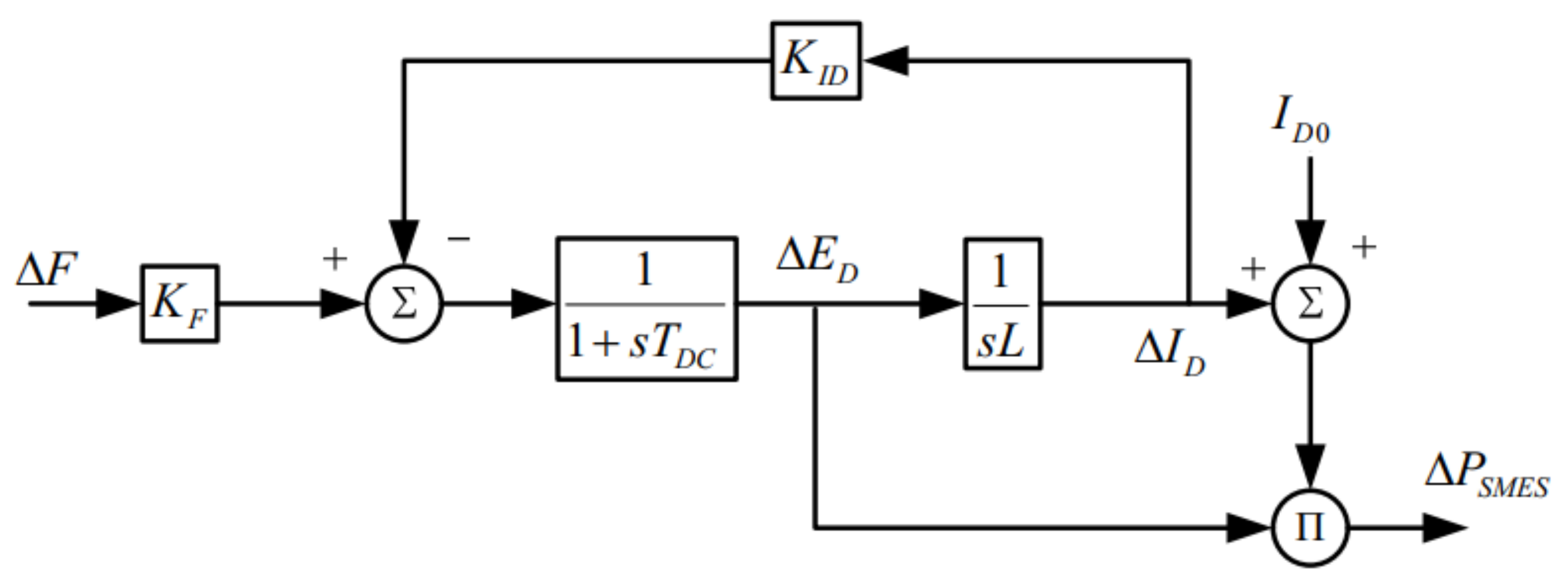
2.3. SMES Configuration

Throughout the regular functioning, charged SMES establishes the value through the system. In case of an unexpected surge in the power requirement, SMES instantly releases the energy stored to accomplish the power demand change. For this duration, it begins the charging instantly, absorbing a certain percentage of the energy which is a surplus to the system [34]. The firing angle $\left(\alpha \right)$ for the converter is furnished by the DC voltage $\left(E_L\right)$ developed at the inductor. The firing angle $\alpha$ changes constantly in a specific range of negative and positive values. When the losses from the converter and the transformer are neglected, the expression for DC voltage may be stated as:

$$E_L=2V_{d0}\cos \alpha -2I_d{R}_c\left\{\begin{array}{c}\mathrm{charging}\mathrm{mode}:\alpha <{90}^{°} \\ \mathrm{discharging}\mathrm{mode}:\alpha >{90}^{°} \end{array}\right.$$

(12)

where $I_d$ denotes the inductor current (kA), $V_{d0}$ denotes the circuit bridge maximum voltage (kV) and $R_C$ denotes commutating resistance (Ω). $E_L$ is constantly monitored with the SMES control loop input signal [34]. Figure 3 shows the SMES unit block diagram. Hence, the variation of $E_L$ and $I_d$ may be expressed as:

$$\mathsf{\Delta }{E}_L=\left(\frac{1}{1+s{T}_{DC}}\right)\left(K_F\mathsf{\Delta }F-K_{ID}\mathsf{\Delta }{I}_D\right)$$

(13)

$$\mathsf{\Delta }{I}_D=\left(\frac{1}{sL}\right)\mathsf{\Delta }{E}_L$$

(14)

where $\mathsf{\Delta }{E}_L$ represents incremental converter voltage deviation (kV), $\mathsf{\Delta }{I}_D$ represents SMES current incremental change (kA), $K_{ID}$ represents $I_D$ feedback gain (kV/kA), $T_{DC}$ represents the time delay of converter (sec), $K_F$ denotes constant of gain (in kV/unit) and L denotes inductance of coil (H). In the time domain, the change in the SMES unit’s real power is represented as:

$$\mathsf{\Delta }{P}_{SMES}=\mathsf{\Delta }{E}_L\left(\mathsf{\Delta }{I}_{D0}+\mathsf{\Delta }{I}_D\right)$$

(15)

In the time domain, the stored energy at any time in the SMES unit is expressed as:

$$W_{SMES}=\frac{I_D^{2}L}{2}$$

(16)

where $K_{ID}$, $K_F$ and $T_{DC}$ are considered as adjustable variables for the definite limits of maximum and minimum.

3. Designing of the System Controller

For the controllers employed in this study, the most vital objectives are to (i) acquire the highest possible power output from the WTG, (ii) control the frequency and power deviation and (iii) manage power among the consumption and production of IHPS. This section depicts the design characterization and execution procedure of the controllers (i.e., conventional or IO-PID, FO-PID, IO-F-PID and FO-F-PID).

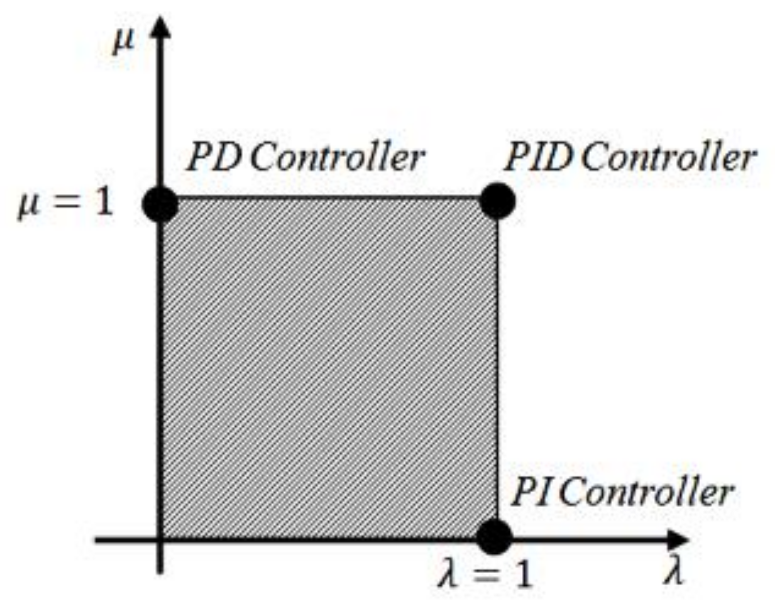
3.1. Essentials of FO Calculus

Fractional calculus is the expansion to the nth-order sequential differentiation and integration (differ-integral) of any random function possessing any real value as its order. The operator for differ-integral is symbolized as ${}_a^{}D{}_b^{\alpha }$, where α (upper limit) ϵ R represents the order of the function a and b (lower limit) are widely employed in fractional calculus.

The differ-integral operator is a single expression to symbolize both the fractional derivative (µ) and integral (λ) [35], expressed as:

$${}_a^{}D{}_b^{\alpha }=\left\{\begin{array}{l}\frac{d^{\alpha }}{d{t}^{\alpha }}\hspace{1em}\hspace{1em}R\left(\alpha \right)>0\\ 1\hspace{1em}\hspace{1em}\hspace{1em}R\left(\alpha \right)=0\\ {{\displaystyle \int }}_a^b{\left(dt\right)}^{-\alpha }\hspace{1em}\hspace{1em}R\left(\alpha \right)<0,\end{array}\right.$$

(17)

Among the most popular definitions of the differ-integral operator (such as definitions by Riemann and Liouville, Grunwald and Letnikov, and Caputo) [15], Riemann and Liouville’s definition for the operator is generally employed [35] and expressed as:

$${}_a^{}D{}_b^{\alpha }f\left(t\right)=\frac{1}{\Gamma \left(m-a\right)}\frac{d^m}{d{t}^m}{{\displaystyle \int }}_a^b\frac{f\left(\tau \right)}{{\left(t-\tau \right)}^{\alpha +1-m}}d\tau$$

(18)

where m is the integer quantity of α, m − 1 < α < m, m ϵ N, Γ(x) is the noted Euler’s gamma function of x and f($\tau$) stands for the related function.

3.2. IO and FO Based PID Controllers

The TF for the simplified PID controller (GC(s)) [16] can be written as:

$$G_C\left(s\right)=\frac{U\left(s\right)}{E\left(s\right)}=K_P+\frac{K_I}{s^{\lambda }}+K_D{s}^{\mu }$$

(19)

where $G_C\left(s\right),E\left(s\right)\mathrm{and}U\left(s\right)$ denote the TF, error signal and the output signal for the controller, respectively; $K_P$ represents proportional controller gain; $K_I$ represents integral controller gain; $K_D$ represents derivative controller gain; and µ and λ represent the differ-integral order operator’s two added variables for designing controllers. In order to obtain the integer-order (IO) controller, µ and λ should be the same or have a value of zero.

By considering variables for the order of differ-integral operator as non-integer, the IO controllers are extended to an FO controller. Hence, the conventional structure of the FO controller holds two independent extra knobs for tuning, i.e., µ and λ, and its IO counterpart. Therefore, some feasible FO controllers are termed as $P{I}^{\lambda }{D}^{\mu }$, $P{I}^{\lambda }$, $P{D}^{\mu }$ and $PI{D}^{\mu }$ controllers.

The schematic view for FO-PID along with the IO-PID controller on the λ-µ plane and justification for the differ-integral operator’s order is presented in Figure 4. The order of the differ-integral operator may vary depending upon its vertical and horizontal axis positioning [36].

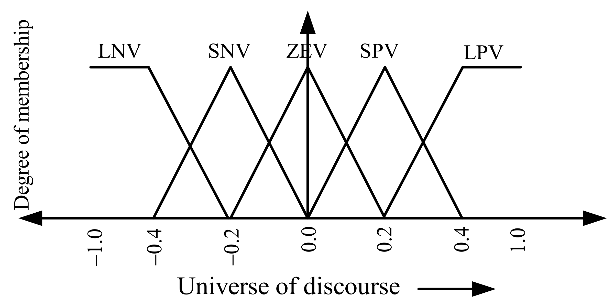
3.3. IO and FO Fuzzy-PID Controllers

Three error signals for the proportional controller (P), integral controller (I) and derivative controller (D) are required for the implementation of the fuzzy-PID controller. These error signals first require fuzzification and later need to be defuzzied in the output signal. More membership functions (MFs) are required for expressively including the entire response curve. However, this will result in a large rule base with regard to its three numbers of input and one number of output-based fuzzy-PID controller. Hence, it becomes difficult to handle such a large rule base. Consequently, the traditional fuzzy-PID controller combines the fuzzy-PI and fuzzy-PD controllers. In this arrangement, the two input scaling factors (SFs) are $K_a$ and $K_b$ and the output SFs are the PI and PD controller gains (Figure 5) [37,38].

In the “IO-F-PID controller”, for FLC, at the input, the order of the rate of change in error as well as at the output order of the integral are integer values (μ = 1 and λ = 1 (Figure 5), respectively). However, this statement does not stand true in the case of the “FO-F-PID controller”; rather, at the input, the order for the rate of change in error as well as at the output order are not integer values but substituted by counterpart fractional numbers (μ, λ). In FLCs, the input-output SFs of a fuzzy controller [37,39] has more effect than tuning the MFs shape for the closed-loop performance. Therefore, in the present study, to attain optimal characteristics with the time domain, the rule base and MFs for the fuzzy controller are assumed as fixed for both “IO-F-PID” and “FO-F-PID” controllers [39]. In addition, more emphasis is put on the input-output SFs (i.e., $K_a$, $K_b$, $K_{PI}$ and $K_{PD}$) for tuning, and in the F-FO-PID controller, μ and λ are tuned. The considered MFs shape and rule base for fuzzy controllers are portrayed in Figure 6 and

Table 1. Considered FLC rule base.

	e	LNV	SNV	ZEV	SPV	LPV
$\frac{{\mathit{d}}^{\mathit{\mu }}\mathit{e}}{\mathit{d}\mathit{t}}$
LPV		ZEV	SPV	LPV	LPV	LPV
SPV		SNV	ZEV	SPV	LPV	LPV
ZEV		LNV	SNV	ZEV	SPV	LPV
SNV		LNV	LNV	SNV	ZEV	SPV
LNV		LNV	LNV	LNV	SNV	ZEV

. The fuzzy linguistic variables depicted in Table 1 such as LNV, SNV, ZEV, SPV and LPV denote a large-negative variable, small-negative variable, zero variable, small-positive variable and large-positive variable, respectively.

4. Performance Index

For enhanced accomplishment of the controller in controlling frequency and power for the Figure 2 system, an optimization method is required. As FLC has non-linear characteristics, there may be no straightforward approach to optimization. The solution lies with the performance indices (such as integral of absolute error (IAE), integral of squared error (ISE), integral of time multiplied absolute error (ITAE) and integral of time multiplied squared error (ITSE)). These four time-domain performance indices are as follows:

$$IAE={{\displaystyle \int }}_0^{\infty }\left|\mathsf{\Delta }\left.F\right|\right.dt$$

(20)

$$ISE={{\displaystyle \int }}_0^{\infty }\left|\mathsf{\Delta }{\left.F\right|}^2\right.dt$$

(21)

$$ITAE={{\displaystyle \int }}_0^{\infty }t\left|\mathsf{\Delta }\left.F\right|\right.dt$$

(22)

$$ITSE={{\displaystyle \int }}_0^{\infty }t\left|\mathsf{\Delta }{\left.F\right|}^2\right.dt$$

(23)

where t represents considered sampling time.

The tuned FLC MFs along with the input-output SFs using a genetic algorithm (GA) to minimize a weighted summation of ISE normalized by maximum error, the maximum percentage of overshoot and the settling time normalized by simulation time. The researchers improved electromagnetism with GA to minimize the ISE while searching for optimal PI^λD^µ parameters. The input-output SFs and differ-integrals of the FO-F-PID controller are tuned while minimizing the weighted sum of various error indices and control signals. The parameter-tuning method of the FO-PID controller is based on GA to find the minimum value of the objective function. To reduce unit step response overshoot, ISE is a more ideal performance criterion; thus, ISE performance criteria were used as the objective function in the design of the controller considering each variable’s limits. Therefore, the problem of designing the system is framed as a constraint problem for optimization, expressed in (24)–(30):

$$Minimize J \left(=ISE\right)$$

(24)

Exposed to the subsequent limits:

(a)

For classical controllers:

$$\left.\begin{array}{l}{K}_{Pj}^{\mathit{min}}\le K_{Pj}\le K_{Pj}^{\mathit{max}}\\ K_{Ij}^{\mathit{min}}\le K_{Ij}\le K_{Ij}^{\mathit{max}}\\ K_{Dj}^{\mathit{min}}\le K_{Dj}\le K_{Dj}^{\mathit{max}}\end{array}\right\}, \hspace{1em}\hspace{1em}\hspace{1em}j=‘W’forWTGand‘D’forDEGunit$$

(25)

(b)

For SMES unit:

$$\left.\begin{array}{l}{K}_{SMES}^{\mathit{min}}\le K_{SMES}\le K_{SMES}^{\mathit{max}}\\ K_{ID}^{\mathit{min}}\le K_{ID}\le K_{ID}^{\mathit{max}}\\ T_{DC}^{\mathit{min}}\le T_{DC}\le T_{DC}^{\mathit{max}}\end{array}\right\}$$

(26)

(c)

For SFs of FLC:

(i)

Input

$$\left.\begin{array}{c}{K}_{aj}^{\mathit{min}}\le K_{aj}\le K_{aj}^{\mathit{max}}\\ K_{bj}^{\mathit{min}}\le K_{bj}\le K_{bj}^{\mathit{max}}\end{array}\right\}\hspace{1em}\hspace{1em}j=1\mathrm{or}2$$

(27)

$$\left.X^{\mu \mathit{min}}\le X^{\mu }\le X^{\mu \mathit{max}}\right\}\hspace{1em}\hspace{1em}\hspace{1em}X=‘W’forWTGand‘D’forDEGunit$$

(28)

(ii)

Output

$$\left.\begin{array}{l}{K}_{PIj}^{\mathit{min}}\le K_{PIj}\le K_{PIj}^{\mathit{max}}\\ K_{PDj}^{\mathit{min}}\le K_{PDj}\le K_{PDj}^{\mathit{max}}\end{array}\right\}\hspace{1em}\hspace{1em}\hspace{1em}j=‘W’forWTGand‘D’forDEGunit$$

(29)

$$\left.X^{{\lambda min}^{{\lambda }^{\lambda max}}}\hspace{1em}\hspace{1em}\hspace{1em}\hspace{1em}X=‘W’ for WTG and ‘D’ for DEG unit\right\}$$

(30)

where $K_P$ represents proportional, $K_I$ represents integral and $K_D$ represents derivative gains of classical controllers; the tunable SMES parameters are $K_{SMES}$, $K_{ID}$ and $T_{DC}$; $K_a$ and $K_b$ are the input of FLC and SF, respectively; and the output of SF and FLC are $K_{PIj}$ and $K_{PDj}$, respectively. From Equations (24)–(30), the minimum and maximum variable values are limited by the min and max range. Here, the QOHS algorithm is utilized for optimization purposes. The output of the optimization program is ISE (i.e., J); at the same time, values are calculated for IAE, ITAE and ITSE performance indices by the optimization program and these obtained values are contended for exhibiting the efficacy of different considered controllers therein [40].

5. Quasi-Oppositional Harmony Search (QOHS) Algorithm

5.1. HS Algorithm

In [25], the authors proposed a novel amendment to the metaheuristic algorithm HS which imitates systematic and natural occurrences. The algorithm is motivated by musicians, analogous to the different combinations of harmony for creating a superior state of harmony and the manner of pitching the instruments. In this algorithm, the obtained solution vector of optimization practice is similar to that of search patterns for the local and global solutions. The distinguishing qualities, such as fewer numerical computations, stochastic random search participation and design to improve vector solution by investigating each prevalent vector solution, contributes to increased reliability and obtaining better solutions for the HS algorithm [41].

The method of optimization for the HS algorithm can ensure better enlightenment through three major measures.

• Initialization: The variables of the algorithm along with the objective function is specified. The initial condition for the harmony memory (HM) may also be defined.
• Harmony improvisation: The novel vector solution is generated by adjusting the pitch and manner of randomization. Additionally, they are associated with the HM vector solution.
• Selection: Until terminating norms are met, the HM continues to find the best solution vector (harmony).

The pseudocode of HS algorithm and the symbols depicted are detailed in [25,28].

5.2. Quasi-Oppositional Learning: A Concept

In [42], to catalyze the convergence rate for an intelligent computational method, the impression of opposition-based learning (OBL) is practiced. Many researchers in their work have reported that the chance of attaining the global optimal vector solution with oppositional vector solution rather than any random vector solution has strong prospects [43]. However, later on, it was demonstrated by Rahnamayan et al. [44] that there is a higher chance of reaching the global best solution with the quasi-opposite points as opposed to opposite points. The definition of the opposite and quasi-opposite numbers along with their respective points as considered for OBL practice and the concept of quasi-opposition is stated in [29,45].

5.3. Quasi-Oppositional Population Initialization

The QOHS algorithm initializes its population arbitrarily like various other population-based optimization algorithms. Even deprived of prior understanding of solution vector(s), with quasi-oppositional learning concepts, better fitting solution vector(s) may be achieved. The structure in this context, as proposed in [29], is as follows:

(a)

initialization of the evenly spread random population;

(b)

establishment of the population with the quasi-opposite learning concept;

(c)

evaluation of the objective function for each variable; and

(d)

best fitting population selection from the early population of a set.

5.4. Quasi-Oppositional Generation Jumping

The present vector of solution compels us to develop a new, healthier solution vector with the application of the evolutionary mechanism [29]. With the assistance of randomization and the pitch adjustment process, a new population is generated, also using the quasi-opposite learning concept, and from the combined population, based on the size of the HM, individuals with higher fitness are chosen [29] considering jumping probability (called jumping rate ($J_r$)). For estimation of the generation jumping of quasi-opposite population, each variable’s opposite and their respective middle points are computed, as explained in [45]. Therefore, with the progress of the search process, there is a decline in the search space range of the different points from the initial limit [29].

5.5. QOHS Algorithm

The pseudo-code of the QOHS algorithm is presented in [29]. Steps 2 and 3 of the algorithm describe HM initialization randomly and with quasi-oppositional concepts, respectively. Quasi-oppositional generation jumping for the QOHS algorithm is presented in Step 6 [29].

6. Simulation and Result Analysis

In this study, to analyze the frequency and power deviations, the IHPS model TF (Figure 2) involving wind and diesel generators along with ESD (i.e., SMES) is taken into consideration. Controlling the actions of the DEG unit through the governor and the WTG unit with the pitch angle is performed by Controllers 1 and 2, respectively, in the considered IHPS TF model (Figure 2). A comparative study based on simulations of the power and frequency deviations of four controllers for the various IHPS model configurations are presented below:

(a)

Controllers 1 and 2 are considered as “PID controller” and the studied model is labelled as “PID”;

(b)

Controllers 1 and 2 are weighted by “FO-PID controller” and the studied model is labelled as “FO-PID”;

(c)

Controllers 1 and 2 are chosen as “IO-F-PID controller” and the studied model is labelled as “IO-F-PID”; and

(d)

Controllers 1 and 2 are realized as “FO-F-PID controller” and the model is labelled as “FO-F-PID”.

In the current study, due to change in load demand, deviations occur in the frequency and power for the IHPS model considered. The QOHS algorithm is utilized for minimizing the objective function value (i.e., J, as expressed in Equation (24)) of various optimizable variables from the ESD and the undertaken controllers, thus restricting the frequency and power deviations. The considered model is analyzed for its performance and robustness. The cases considered are listed below.

• Performance Analysis
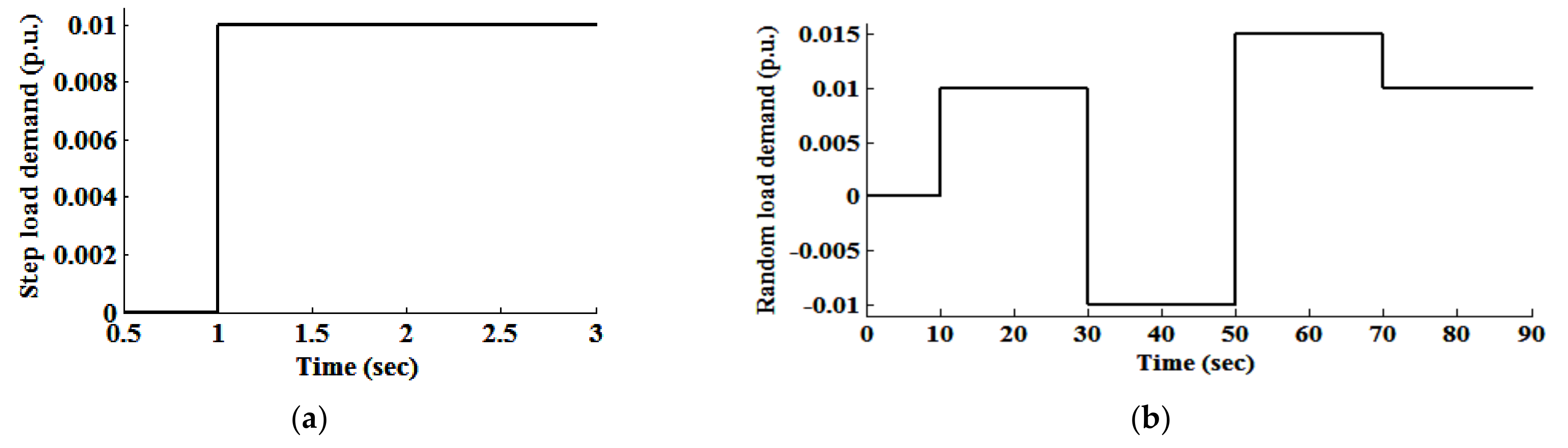
  • Case I: Analyze the functioning for input load demand of 1% step
  • Case II: Analyze the functioning for input random load demand
• Rate Constraint type
  • Case III: Rate constraint type non-linear ESD operation
  • Case IV: Rate constraint type non-linear DEG operation
• Effect of loading mismatch
  • Case V: Lesser loading state
  • Case VI: Higher loading state

Different input perturbations are depicted in Figure 7 for (a) step and (b) random load demand for the present simulation work. Step load demand is operated at t = 1 s (Figure 7a), whereas random load demand is operated at t = 10, 30, 50 and 70 s (Figure 7b). The most significant observations of the present work are detailed in the following sections. In the corresponding tables, the findings with concern are marked as bold.

6.1. Performance Analysis of Different Controller-Based Configurations

In this segment, the performances of different configurations for the controllers (“PID”, “FO-PID”, “IO-F-PID” and “FO-F-PID”) in the time domains of the IHPS model are analyzed. Two different conditions are considered for the analytical performance study, and the assessments of the relative performance under different cases for the considered IHPS model for four types of controllers are presented. The QOHS algorithm is employed for each case and every controller type for the optimal controller parameters.

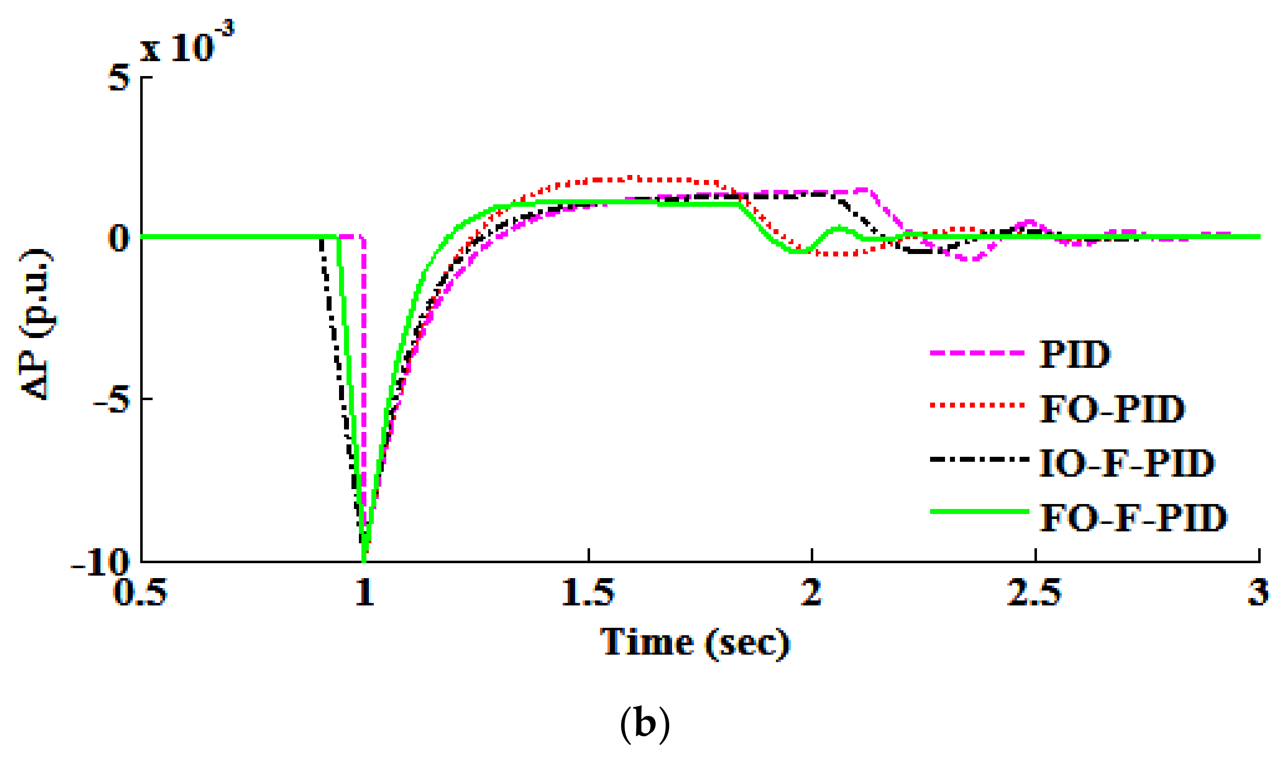
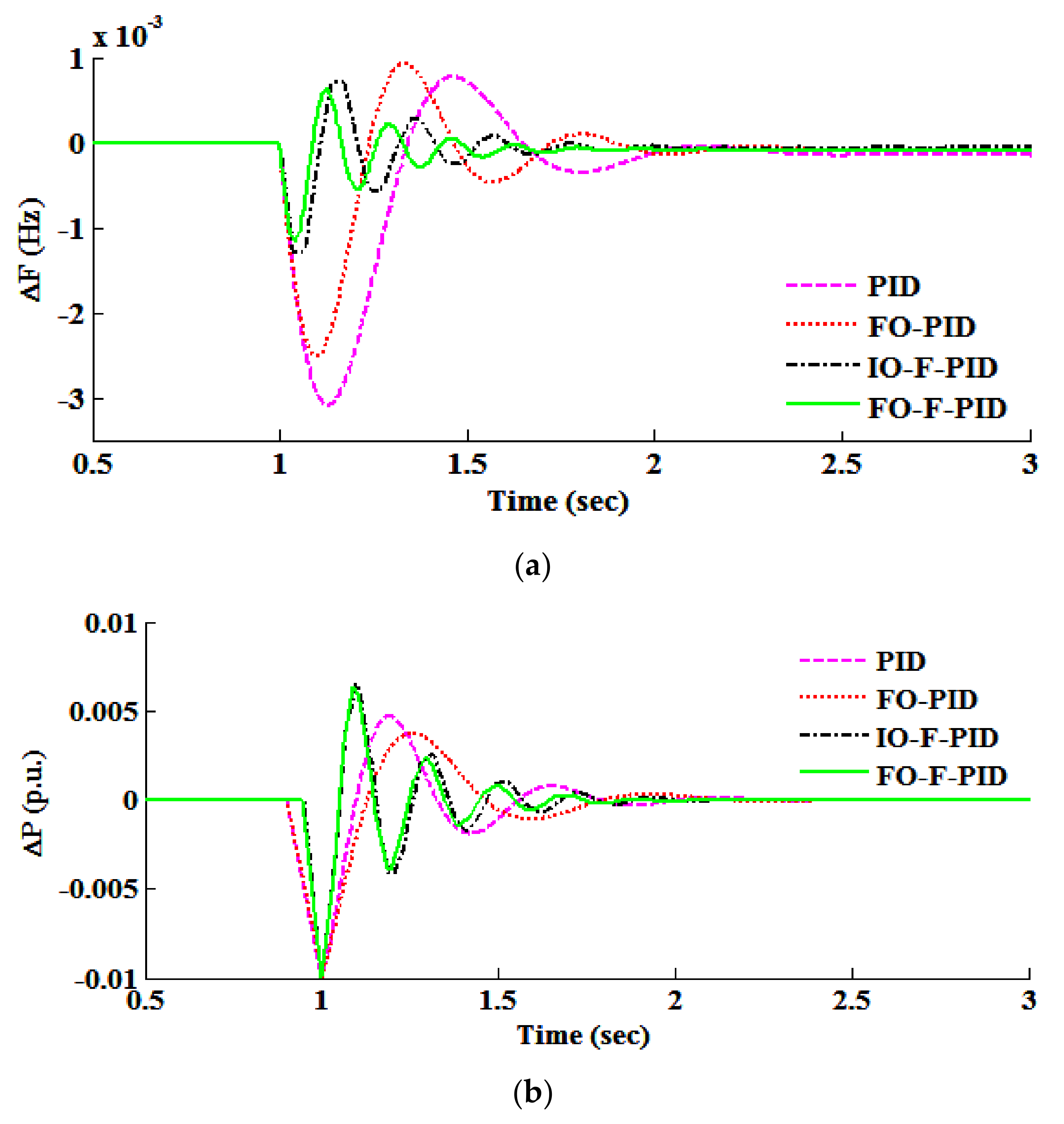
6.1.1. Case Study I: Performance Analysis for 1% Step Input Load Demand Condition

For performance analysis of the four distinct configurations of the IHPS model (“PID”, “FO-PID”, “IO-F-PID” and “FO-F-PID”), a 1% step abrupt increment in demand load is operated at t = 1 s (Figure 7a). The related results of frequency and power deviation are exhibited in Figure 8. The optimal gains are represented in

Table 2. “IO-F-PID” and “FO-F-PID” optimizable variables of IHPS for DEG and WTG controllers along with the SMES block.

Unit	Parameters	Various Configurations of IHPS with Load Type
		PID		FO-PID
Gains of Different Controllers		Step	Random	Step	Random
WTG	KPW	0.3705	13.5215	16.0379	4.5142
	KIW	1.0086	26.6082	11.0892	4.3424
	KDW	0.5738	4.0462	1.0083	4.1194
	Wµ	1.0	1.0	0.3323	0.5218
	Wλ	1.0	1.0	0.4199	0.6462
DEG	KPD	1.0673	34.3797	3.3648	12.9453
	KID	1.0296	14.4839	18.7786	25.9908
	KDD	1.0264	4.2786	0.0248	10.3135
	Dµ	1.0	1.0	0.6307	0.8277
	Dλ	1.0	1.0	0.2159	0.9191
SMES block	KSMES	98.8751	78.5629	82.4721	95.8835
	TDC (sec)	0.1243	0.0294	0.0368	0.2663
	KID	0.2699	0.7064	0.2857	0.0778

and

Table 3. “IO-F-PID” and “FO-F-PID” optimizable variables of IHPS for DEG and WTG controllers along with the SMES block.

Unit	Parameters	Various Configurations of IHPS with Load Type
		IO-F-PID		FO-F-PID
Gains of Different Controllers		Step	Random	Step	Random	Case V
WTG	Ka1	0.8954	0.9813	0.5708	0.4462	0.7036
	Kb1	0.5092	0.6532	0.6291	0.1092	0.7553
	KPIW	5.4566	4.3456	3.9421	2.1884	4.3827
	KPDW	0.6651	0.8108	23.899	2.7175	2.3244
	Wµ	1.00	1.00	0.5273	1.0554	1.0447
	Wλ	1.00	1.00	0.9789	0.6416	0.5466
DEG	Ka2	0.2164	0.9291	1.0264	0.5513	0.9432
	Kb2	0.0553	0.7134	0.9207	0.5419	0.8003
	KPID	9.9449	2.8693	0.8971	0.579	10.826
	KPDD	0.9106	2.7937	27.254	2.3813	2.5427
	Dµ	1.00	1.00	1.0054	0.3507	0.8342
	Dλ	1.00	1.00	0.8203	0.5407	0.8754
SMES block	KSMES	99.589	71.408	84.631	94.805	99.965
	TDC (sec)	0.2673	0.0496	0.2542	0.1086	0.2395
	KID	2.2253	0.0605	2.4085	0.3194	2.1828

of the controllers and the SMES unit for diverse IHPS model configuration under a 1% rise in the demand load. It can be observed from Figure 8 that the IHPS configurations based on the FO controller (i.e., “FO-PID” and “FO-F-PID”) have an advantage over the controller configurations based on IO (i.e., “PID” and “IO-F-PID”) in terms of maximum overshoot (Mp) (i.e., less Mp) and less settling time (ts). Through the inclusive assessment, the “FO-F-PID” configuration is confirmed as the most effective in terms of $t_s$ and $M_P$ and is established as superior to the other three configurations. Additionally, the report regarding the frequency deviation under the transient state (from the plots obtained for different configurations) is presented in

Table 4. Transient characteristic assessment and performance indices for various configurations based on controllers used in Case I (i.e., 1% load demand step increase).

Controller Type	System Parameter	Mp (×10−3)	tr (sec)	ts (sec)	Ess (×10−4)	IAE (×10−4)	ISE (×10−7)	ITSE (×10−7)	ITAE (×10−4)
PID	ΔF	0.859	0.398	1.425	8.703	2.279	1.217	3.677	4.673
FO-PID	ΔF	0.579	0.382	1.153	5.806	1.777	1. 108	3.004	3.957
IO-F-PID	ΔF	0.447	0.429	0.896	3.687	0.956	0.871	2.285	3.278
FO-F-PID	ΔF	0.344	0.417	0.764	1.585	0.851	0.629	2.289	2.810

, representing the individual controller-based IHPS models. Table 4 confirms the “FO-F-PID” configuration’s improved results in terms of controlling the variation in power and frequency over the other considered configurations. In addition, in Table 4, the objective function value (J = ISE) and the generated values for the remaining three performance indices are depicted. It can be observed that the “FO-F-PID” configuration of the IHPS has the lowest values for the performance indices as well as for the objective function. This endorses the character of responses depicted in Figure 8 (i.e., nature of response for various undertaken IHPS model configurations).

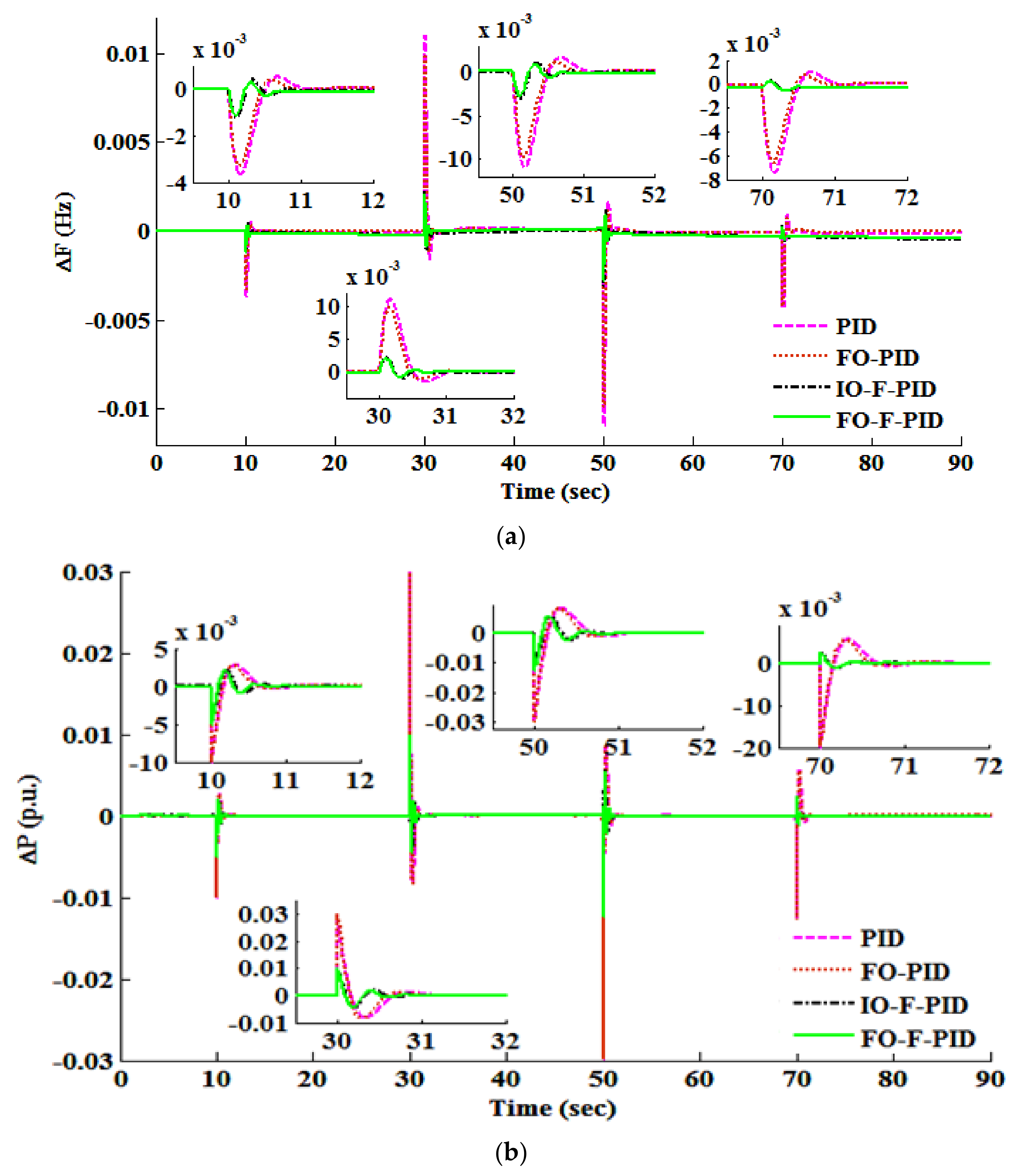
6.1.2. Case Study II: Performance Analysis under Random Load Demand Condition

To verify the characteristics of various configurations of the undertaken IHPS model under the practical ecosystem, the different configurations were exposed to a randomly varying load demand (Figure 7b). Here, to obtain the optimized parameters against diverse controller configurations and SMES parameters, the QOHS algorithm is utilized. Figure 9a,b depict the results of the acquired deviation for the frequency and power of each IHPS model configuration for the variation of random load. At the same time, control over the system and dominating the power and frequency deviation at the earliest after every variation in load can be observed (Figure 9), in which the IHPS model with “FO-F-PID” configuration has an edge over the other considered configurations (i.e., “PID”, “FO-PID” and “IO-F-PID”).

The controller gain parameters optimized with the QOHS algorithm for the considered configurations and tunable SMES parameters with the studied case are shown in Table 2 and Table 3. In addition, a zoomed-in view of the deviation in power and frequency is displayed in Figure 9, depicting, with additional transparency, the nature of every IHPS configuration in terms of ts, steady-state error (Ess) and Mp (i.e., less Mp).

6.2. Robustness Analysis of Different Controller-Based Configurations

In this study, to validate the robustness of the QOHS algorithm and FO controller, two categories of investigation were carried out with the undertaken configurations of the IHPS model. In the first investigation, significant nonlinearity was introduced [46] under the practice of incorporating rate constraint nature in the DEG unit or ESD of the model. During the second investigation, a mismatch for the demand load was instigated with the optimally adjusted variables, designed to study the robustness of the considered IHPS. The first method (i.e., non-linearity by rate constraint) limits specific source energy from accumulating or discharging energy immediately by establishing an upper and lower boundary, which can be regarded as strongly resembling a more practical situation. The application of the non-linearity of rate constraint with the first-order TF is shown in Figure 10.

6.2.1. Case Study III: Rate Constraint Type Non-Linear ESD Operation

For Case Study III, all the configurations undertaken for the study of the IHPS model have been taken into consideration for a robustness study. In the same vein, the non-linearity block is formulated under the SMES block in Figure 2. In the SMES block, a non-linearity component is inserted considering rate constraint (Figure 10) with a value of $\left|P_{SMES}\right|$ < 0.005. The controllers gain variables and the tunable SMES parameters, which are optimized by the QOHS algorithm for the linear operation.

The performance of the IHPS model’s every configuration and the SMES configuration in conjunction with non-linearity in the form of rate constraint under an abrupt increase in load demand in step manner is presented in Figure 11 along with the change in the frequency and power. It can be observed that FO controllers have an edge over the IO controllers. The IHPS model with the FO-F-PID controller proved its competency over the other controllers (PID, FO-PID and IO-F-PID) in controlling the abrupt shift in load (Figure 11). The transient performance analyses through simulation (Figure 11) are presented in

Table 5. Transient characteristic assessment and performance indices for various configurations based on the controller used in Case III (i.e., rate constraint type non-linearity of ESD).

Controller Type	System Parameter	Mp (×10−3)	tr (sec)	ts (sec)	Ess (×10−4)	IAE (×10−4)	ISE (×10−7)	ITSE (×10−7)	ITAE (×10−4)
PID	ΔF	0.205	1.192	1.755	0.877	3.726	1.275	1.811	6.099
FO-PID	ΔF	0.148	1.132	1.535	0.942	2.248	0.499	0.659	4.326
IO-F-PID	ΔF	0.325	0.921	1.415	0.521	3.709	1.166	1.656	6.519
FO-F-PID	ΔF	0.019	0.884	1.167	0.495	3.717	0.128	0.181	6.064

.

.

6.2.2. Case Study IV: Rate Constraint Type Non-Linear DEG Operation

In Case Study IV, the DEG unit non-linearity in the form of rate constraint (Figure 10) is presented, as depicted in Figure 2. Its variation in power and frequency for the various considered configurations of the IHPS model (“PID”, “FO-PID”, “IO-F-PID” and “FO-F-PID”) are presented in Figure 12 for a load variation with an abrupt increase (Figure 7a). The value employed regarding the rate constraint type is $\left|P_{DEG}\right|$ < 0.001. Considering the various sub-plots associated with Figure 12, the situation revealed that an improved controlling nature may be obtained with FO controllers over IO controllers under the non-linearity effect consideration. The HIPS model with the “FO-F-PID” configuration has an edge over the remaining three configurations (“PID”, “FO-PID” and “IO-F-PID”) during unexpected deviations in load demand with non-linearity at the DEG unit in the form of rate constraint. Figure 12 shows the nature of transient performance and

Table 6. Transient characteristic assessment and performance indices for various configurations based on the controller used in Case IV (i.e., rate constraint type non-linearity of DEG).

Controller Type	System Parameter	Mp (×10−3)	tr (sec)	ts (sec)	Ess (×10−4)	IAE (×10−4)	ISE (×10−7)	ITSE (×10−7)	ITAE (×10−4)
PID	ΔF	0.763	0.392	1.367	1.516	3.132	2.741	8.447	9.978
FO-PID	ΔF	0.931	0.288	1.163	1.021	3.099	2.595	8.114	9.596
IO-F-PID	ΔF	0.725	0.138	0.946	0.633	2.262	1.331	3.938	6.828
FO-F-PID	ΔF	0.620	0.108	0.791	0.947	1.864	1.263	2.121	5.295

depicts the performance indices conceded.

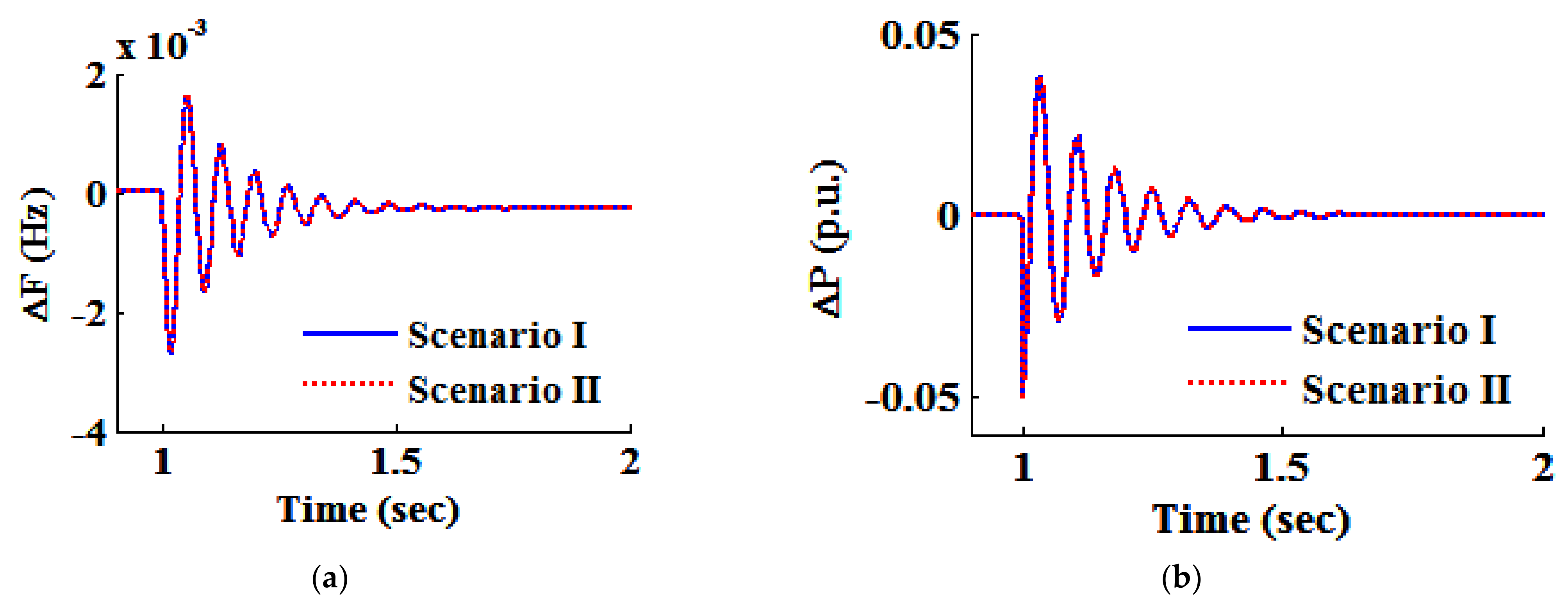
6.2.3. Case Study V: Lesser Loading State

For the analysis of the robustness of the system with loading mismatch, optimization is achieved for the controllers’ gains (positioned on the side of the DEG and the WTG) along with the SMES optimizable variables with the QOHS algorithm for 90% of the loading ability. In this case, if there is a loading mismatch, the system is loaded only to 85% loading ability. Therefore, robustness evaluation for the present case is carried out in consideration of the two scenarios, as depicted in

Table 7. Robustness assessment of Case V scenarios.

Scenario	Loading Consideration under Parameter Optimization	Practical Loading
I	90.00%	90.00%
II	90.00%	85.00%

.

The optimized gains for Controller 1 and Controller 2 are offered at Table 3 along with the SMES block variables for the IHPS model under the “FO-F-PID” configuration as achieved with the QOHS algorithm. The comparative profiles for the deviation in the frequency and power of the analyzed FO-F-PID controller in accordance with the IHPS model under Scenario I and Scenario II are presented in Figure 13a,b. Figure 13 demonstrates that the deviation profile for the frequency and the power in the two considered scenarios are overlapping, which offers robust optimization of the FO-F-PID controller through the QOHS algorithm. Information related to transience and the distinguished impact of the current work for both the considered scenarios is exhibited in

Table 8. Transient characteristics assessment for the undertaken scenarios of Case V and Case VI with deviation in frequency.

Considered Case	Scenario	Frequency Deviation	Mp (×10−3)	Ess (×10−4)	tr (sec)	ts (sec)
Case V	Scenario I	ΔF	1.619	2.775	0.054	0.63
	Scenario II	ΔF	1.617	2.775	0.054	0.63
Case VI	Scenario I	ΔF	1.619	2.775	0.054	0.63
	Scenario II	ΔF	1.621	2.775	0.054	0.63

.

6.2.4. Case Study VI: Higher Loading Mismatch State

Case Study VI is characterized by 95% system loading capacity, and the associated FO-F-PID controller gains for DEG, WTG along with SMES tunable variables are optimized for the capacity of 90% loading. Hence, in

Table 9. Robustness assessment of Case VI scenarios.

Scenario	Loading Consideration under Parameter Optimization	Practical Loading
I	90.00%	90.00%
II	90.00%	95.00%

, the robustness assessment on this case is shown by considering both situations.

The QOHS algorithm as well as the FO-F-PID controller’s robustness can be easily verified with assistance from Figure 14a,b under both considered scenarios for the deviation in frequency and strength with the FO-F-PID controller-based IHPS model. Table 3 depicts the FO-F-PID controller’s optimal values and the adjustable variables from SMES for a sudden 10% load demand increase in step manner (same as Case V). Figure 14 depicts the two different scenarios as having identical responses, confirming the QOHS algorithm’s robustness for optimizing the adjustable variables. The dissimilarity between the situations is represented in Table 8 in the manner of transient data for the generated characteristics of transient nature.

7. Conclusions

In the present study, challenges such as (a) the overemployment of DEG systems for electrification, (b) fossil fuel rapid exhaustion, (c) countryside electrification and (d) global warming are foreseen and solved with a trustworthy and controlled inexhaustible energy source based on IHPS. The following outcomes are achieved with various system configurations:

(a)

For the studied IHPS, the hybridized classical fuzzy controller using the concept of FO of calculus is projected and the discrete system configurations framed are labelled as “PID”, “FO-PID”, “IO-F-PID” and “FO-F-PID”.

(b)

The FO concept applied in the controllers upholds its capability in governing the dynamics of the system.

(c)

For the IHPS application, the priority is to set up a static configuration for MF and the rule base of FLCs.

(d)

In the context of the considered associated power engineering problems, the utilization of the QOHS scheme proves to be effective in generating close proximity to the global optimal solution.

(e)

For the studied IHPS model, the “FO-PID” configuration’s performance and robustness are no less than that of the “IO-F-PID” arrangement.

(f)

In governing the deviations for both power and frequency in rate constraint-centered robustness analysis, the FO controllers proved their effectiveness and were found to be more competitive compared to the IO controller.

(g)

The complete performance and robustness analysis conclude that under the changing load conditions, the “FO-F-PID” controller is the most effective in limiting the changes for both power and frequency, followed by “IO-F-PID”, “FO-PID” and “PID” controllers.

References

1. Nock, D.; Levin, T.; Baker, E. Changing the policy paradigm: A benefit maximization approach to electricity planning in developing countries. Appl. Energy 2020, 264, 114583. [Google Scholar] [CrossRef]
2. Kirubi, C.; Jacobson, A.; Kammen, D.M.; Mills, A. Community-Based Electric Micro-Grids Can Contribute to Rural Development: Evidence from Kenya. World Dev. 2009, 37, 1208–1221. [Google Scholar] [CrossRef]
3. Kaabeche, A.; Ibtiouen, R. Techno-economic optimization of hybrid photovoltaic/wind/diesel/battery generation in a stand-alone power system. Sol. Energy 2014, 103, 171–182. [Google Scholar] [CrossRef]
4. Byrne, J.; Shen, B.; Wallace, W. The economics of sustainable energy for rural development: A study of renewable energy in rural China. Energy Policy 1998, 26, 45–54. [Google Scholar] [CrossRef]
5. Bajpai, P.; Dash, V. Hybrid renewable energy systems for power generation in stand-alone applications: A review. Renew. Sustain. Energy Rev. 2012, 16, 2926–2939. [Google Scholar] [CrossRef]
6. Holttinen, H.; Hirvonen, R. Power System Requirements for Wind Power; John Wiley & Sons: Hoboken, NJ, USA, 2005. [Google Scholar]
7. Sebastián, R.; Castro, M.; Sancristobal, E.; Yeves, F.; Peire, J.; Quesada, J. Approaching hybrid wind-diesel systems and controller area network. IECON Proc. Ind. Electron. Conf. 2002, 3, 2300–2305. [Google Scholar]
8. Li, W.; Joós, G. Comparison of energy storage system technologies and configurations in a wind farm. In Proceedings of the PESC Rec. IEEE Annual Power Electronics Specialists Conference, Orlando, FL, USA, 17–21 June 2007; pp. 1280–1285. [Google Scholar]
9. Tripathy, S.C.; Kalantar, M.; Balasubramanian, R. Dynamics and Stability of Wind and Diesel Turbine Generators with Superconducting Magnetic Energy Storage Unit on an Isolated Power System. IEEE Trans. Energy Convers. 1991, 6, 579–585. [Google Scholar] [CrossRef]
10. Senjyu, T.; Hayashi, D.; Urasaki, N.; Funabashi, T. Oscillation frequency control based on H∞ controller for a small power system using renewable energy facilities in isolated island. In Proceedings of the 2002 IEEE Power Engineering Society General Meeting, Tokyo, Japan, 18–22 June 2002; pp. 117–124. [Google Scholar]
11. Simoes, M.G.; Bose, B.K.; Spiegel, R.J. Design and performance evaluation of a fuzzy-logic-based variable-speed wind generation system. IEEE Trans. Ind. Appl. 1997, 33, 956–965. [Google Scholar] [CrossRef] [Green Version]
12. Zadeh, L.A. Fuzzy sets. Inf. Control 1965, 8, 338–353. [Google Scholar] [CrossRef] [Green Version]
13. Li, W. Design of a hybrid fuzzy logic proportional plus conventional integral-derivative controller. IEEE Trans. Fuzzy Syst. 1998, 6, 449–463. [Google Scholar] [CrossRef] [Green Version]
14. Carvajal, J.; Chen, G.; Ogmen, H. Fuzzy PID controller: Design, performance evaluation, and stability analysis. Inf. Sci. 2000, 123, 249–270. [Google Scholar] [CrossRef]
15. Das, S. Functional Fractional Calculus for System Identification and Controls; Springer: Berlin/Heidelberg, Germany, 2008. [Google Scholar]
16. Podlubny, I. Fractional-order systems and PIλDµ-controllers. IEEE Trans Autom. Control 1999, 44, 208–214. [Google Scholar] [CrossRef]
17. Melício, R.; Mendes, V.M.F.; Catalão, J.P.S. Fractional-order control and simulation of wind energy systems with PMSG/full-power converter topology. Energy Convers. Manag. 2010, 51, 1250–1258. [Google Scholar] [CrossRef]
18. Das, S.; Pan, I.; Das, S. Fractional order fuzzy control of nuclear reactor power with thermal-hydraulic effects in the presence of random network induced delay and sensor noise having long range dependence. Energy Convers. Manag. 2013, 68, 200–218. [Google Scholar] [CrossRef] [Green Version]
19. Chen, Z.; Yuan, X.; Ji, B.; Wang, P.; Tian, H. Design of a fractional order PID controller for hydraulic turbine regulating system using chaotic non-dominated sorting genetic algorithm II. Energy Convers. Manag. 2014, 84, 390–404. [Google Scholar] [CrossRef]
20. Das, S.; Pan, I.; Das, S. Performance comparison of optimal fractional order hybrid fuzzy PID controllers for handling oscillatory fractional order processes with dead time. ISA Trans. 2013, 52, 550–566. [Google Scholar] [CrossRef] [Green Version]
21. Das, S.; Pan, I.; Das, S.; Gupta, A. A novel fractional order fuzzy PID controller and its optimal time domain tuning based on integral performance indices. Eng. Appl. Artif. Intell. 2012, 25, 430–442. [Google Scholar] [CrossRef] [Green Version]
22. Pan, I.; Das, S. Chaotic multi-objective optimization based design of fractional order PI λD μ controller in AVR system. Int. J. Electr. Power Energy Syst. 2012, 43, 393–407. [Google Scholar] [CrossRef] [Green Version]
23. Pan, I.; Das, S. Fractional-order load-frequency control of interconnected power systems using chaotic multi-objective optimization. Appl. Soft Comput. J. 2015, 29, 328–344. [Google Scholar] [CrossRef] [Green Version]
24. Pan, I.; Das, S. Kriging based surrogate modeling for fractional order control of microgrids. IEEE Trans. Smart Grid 2015, 6, 36–44. [Google Scholar] [CrossRef] [Green Version]
25. Geem, Z.W.; Kim, J.H.; Loganathan, G.V. A new heuristic optimization algorithm: Harmony search. Simulations 2001, 76, 60–68. [Google Scholar] [CrossRef]
26. Omran, M.G.H. Global-best harmony search. Appl. Math. Comput. 2008, 198, 643–656. [Google Scholar] [CrossRef]
27. Mahdavi, M.; Fesanghary, M.; Damangir, E. An improved harmony search algorithm for solving optimization problems. Appl. Math. Comput. 2007, 188, 1567–1579. [Google Scholar] [CrossRef]
28. Banerjee, A.; Mukherjee, V.; Ghoshal, S.P. An opposition-based harmony search algorithm for engineering optimization problems. Ain Shams Eng. J. 2014, 5, 85–101. [Google Scholar] [CrossRef] [Green Version]
29. Tarkeshwar, M.; Mukherjee, V. Quasi-oppositional harmony search algorithm and fuzzy logic controller for load frequency stabilisation of an isolated hybrid power system. IET Gener. Transm. Distrib. 2015, 9, 427–444. [Google Scholar] [CrossRef]
30. Bhatti, T.S.; Al-Ademi, A.A.F.; Bansal, N.K. Load frequency control of isolated wind diesel hybrid power systems. Energy Convers. Manag. 1997, 38, 829–837. [Google Scholar] [CrossRef]
31. Yang, H.; Wei, Z.; Chengzhi, L. Optimal design and techno-economic analysis of a hybrid solar-wind power generation system. Appl. Energy 2009, 86, 163–169. [Google Scholar] [CrossRef]
32. Ismail, M.S.; Moghavvemi, M.; Mahlia, T.M.I. Techno-economic analysis of an optimized photovoltaic and diesel generator hybrid power system for remote houses in a tropical climate. Energy Convers. Manag. 2013, 69, 163–173. [Google Scholar] [CrossRef]
33. Sedaghat, B.; Jalilvand, A.; Noroozian, R. Design of a multilevel control strategy for integration of stand-alone wind/diesel system. Int. J. Electr. Power Energy Syst. 2012, 35, 123–137. [Google Scholar] [CrossRef]
34. Tripathy, S.C.; Balasubramanian, R.; Nair, P.S.C. Effect of Superconducting Magnetic Energy Storage on Automatic Generation Control Considering Governor Deadband and Boiler Dynamics. IEEE Trans. Power Syst. 1992, 7, 1266–1273. [Google Scholar] [CrossRef]
35. Monje, C.A.; Chen, Y.Q.; Vinagre, B.M.; Xue, D.; Feliu-Batlle, V. Fractional-Order Systems and Controls: Fundamentals and Applications; Springer: London, UK, 2010. [Google Scholar]
36. Maiti, D.; Biswas, S.; Konar, A. Design of a fractional order PID controller using particle swarm optimization technique. In Proceedings of the 2nd National Conference on Recent Trends in Information Systems, Jadavpur University, Kolkata, India, 9–11 July 2015; pp. 1–5. [Google Scholar]
37. Mudi, R.K.; Pal, N.R. A robust self-tuning scheme for PI- and PD-type fuzzy controllers. IEEE Trans. Fuzzy Syst. 1999, 7, 2–16. [Google Scholar] [CrossRef] [Green Version]
38. Yeşil, E.; Güzelkaya, M.; Eksin, I. Self tuning fuzzy PID type load and frequency controller. Energy Convers. Manag. 2004, 45, 377–390. [Google Scholar] [CrossRef]
39. Woo, Z.W.; Chung, H.Y.; Lin, J.J. A PID type fuzzy controller with self-tuning scaling factors. Fuzzy Sets Syst. 2000, 115, 321–326. [Google Scholar] [CrossRef]
40. Banerjee, A.; Mukherjee, V.; Ghoshal, S.P. Modeling and seeker optimization based simulation for intelligent reactive power control of an isolated hybrid power system. Swarm Evol. Comput. 2013, 13, 85–100. [Google Scholar] [CrossRef]
41. Yang, X.S.; Geem, Z.W. Harmony Search as a Metaheuristic Algorithm. In Music-Inspired Harmony Search Algorithm: Theory and Applications; Studies in Computational Intelligence; Springer: Berlin/Heidelberg, Germany, 2009; Volume 191, pp. 1–14. [Google Scholar]
42. Tizhoosh, H.R. Opposition-based learning: A new scheme for machine intelligence. In Proceedings of the International Conference on Intelligent Agents, Web Technologies and Internet, CIMCA, Vienna, Austria, 28–30 November 2005; Volume 1, pp. 695–701. [Google Scholar]
43. Rahnamayan, S.; Tizhoosh, H.R.; Salama, M.M.A. Opposition versus randomness in soft computing techniques. Appl. Soft Comput. J. 2008, 8, 906–918. [Google Scholar] [CrossRef]
44. Rahnamayan, S.; Tizhoosh, H.R.; Salama, M.M.A. Quasi-oppositional differential evolution. In Proceedings of the 2007 IEEE Congress on Evolutionary Computation, CEC 2007, Singapore, 25–28 September 2007; pp. 2229–2236. [Google Scholar]
45. Chatterjee, A.; Ghoshal, S.P.; Mukherjee, V. Solution of combined economic and emission dispatch problems of power systems by an opposition-based harmony search algorithm. Int. J. Electr. Power Energy Syst. 2012, 39, 9–20. [Google Scholar] [CrossRef]
46. Wang, Y.; Zhou, R.; Wen, C. Robust load-frequency controller design for power systems. IEE Proc. C Gener. Transm. Distrib. 1993, 140, 11–16. [Google Scholar] [CrossRef]
Figure 1. A flow chart representation of the present work in a step-by-step manner.
Energies 14 06459 g001
Figure 2. Schematic structural depiction of the undertaken IHPS.
Energies 14 06459 g002
Figure 3. Schematic structure of the SMES unit.
Energies 14 06459 g003
Figure 4. Interpretation of FO-PID and IO-PID controller.
Energies 14 06459 g004
Figure 5. Structural representation of FO-F-PID controller.
Energies 14 06459 g005
Figure 6. FLC membership functions for the error signal, the fractional derivative of the error signal and output signal.
Energies 14 06459 g006
Figure 7. Various considered load demands profiles: (a) step increase by 1% and (b) random.
Energies 14 06459 g007
Figure 8. For the considered configurations of IHPS concerning Case I (i.e., 1% step increase in loading condition), the performance compression of (a) Δ F H z and (b) Δ P p . u . .
Energies 14 06459 g008
Figure 9. For considered configurations of IHPS concerning Case II (i.e., random load disturbance condition), the performance compression of (a) Δ F H z and (b) Δ P p . u . .
Energies 14 06459 g009
Figure 10. Non-linearity in the form of rate constraint for the energy storage and generator unit with first-order TF representation in the feedback path.
Energies 14 06459 g010
Figure 11. For considered configurations of IHPS concerning Case III (i.e., 1% step increase in load demand with rate constraint type non-linear operation on the SMES), the performance compression (a) Δ F H z and (b) Δ P p . u . .
Energies 14 06459 g011aEnergies 14 06459 g011b
Figure 12. For the considered configurations of IHPS concerning Case IV (i.e., 1% step increase in load demand with rate constraint type non-linear operation on the DEG), the performance compression of (a) Δ F H z and (b) Δ P p . u . .
Energies 14 06459 g012
Figure 13. Considered scenarios of “FO-F-PID” formulation of IHPS concerning Case V, performance compression of (a) ∆F (Hz) and (b) ∆P (p.u.).
Energies 14 06459 g013
Figure 14. Considered scenarios of “FO-F-PID” formulation of IHPS concerning Case VI, performance compression of (a) ∆F (Hz) and (b) ∆P (p.u.).
Energies 14 06459 g014